GLOBAL ASYMPTOTIC SOLUTIONS FOR
RELATIVISTIC MHD JETS AND WINDS

Abstract

We consider relativistic, stationary, axisymmetric, polytropic, unconfined, perfect MHD winds, assuming their five lagrangian first integrals to be known. The asymptotic structure consists of field-regions bordered by boundary layers along the polar axis and at null surfaces, such as the equatorial plane, which have the structure of charged column or sheet pinches supported by plasma or magnetic poloidal pressure. In each field-region cell, the proper current (defined here as the ratio of the asymptotic poloidal current to the asymptotic Lorentz factor) remains constant. Our solution is given in the form of matched asymptotic solutions separately valid outside and inside the boundary layers. An Hamilton-Jacobi equation, or equivalently a Grad-Shafranov equation, gives the asymptotic structure in the field-regions of winds which carry Poynting flux to infinity. An important consistency relation is found to exist between axial pressure, axial current and asymptotic Lorentz factor. We similarly derive WKB-type analytic solutions for winds which are kinetic-energy dominated at infinity and whose magnetic surfaces focus to paraboloids. The density on the axis in the polar boundary column is shown to slowly fall off as a negative power of the logarithm of the distance to the wind source. The geometry of magnetic surfaces in all parts of the asymptotic domain, including boundary layers, is explicitly deduced in terms of the first-integrals.

1 Introduction

Any stationary axisymmetric non-relativistic, rotating, magnetized wind will collimate at large distances from the source, under perfect MHD conditions and polytropic thermodynamics (Heyvaerts & Norman, 1989). Chiueh et al. (1991) showed that these results hold also for relativistic winds. We have recently extended our general analysis (Heyvaerts & Norman, 2002a) by presenting global analytic asymptotic solutions for non-relativistic winds, valid from the pole to the equator, assuming given first integrals. This paper extends our general analysis to relativistic winds.

Flows which bring no Poynting flux to infinity are called kinetic winds. Their magnetic surfaces asymptote to paraboloids (Heyvaerts & Norman (1989), Chiueh et al. (1991)). If Poynting flux reaches infinity, the flow is called a Poynting jet. The magnetic surfaces then asymptotically approach cylinders or conical surfaces in which cylindrical ones are nested. We refer to a magnetic surface as being asymptotically conical if both $r$ and $z$ approach infinity on this magnetic surface, such that $(z/r)$ approaches a finite value.

We find that the asymptotic structure of relativistic winds consists of field-regions where the Lorentz force vanishes in the direction normal to magnetic surfaces. These regions are bounded by null surfaces where the magnetic field vanishes. In the vicinity of null surfaces, the plasma pressure, or possibly the poloidal magnetic pressure, is significant. The vicinity of the polar axis is also a boundary layer region.

Relativistic winds are likely to be present near pulsars, active galactic nuclei, microquasars and gamma ray burst sources. Their structure has been first discussed assuming conical magnetic surfaces (Michel (1969), Goldreich & Julian (1970)). The cross field force balance has been considered by Okamoto (1975) and Heinemann & Olbert (1978). It has then been recognized that both non-relativistic and relativistic winds focus asymptotically (Blandford & Payne (1982), Heyvaerts & Norman (1989), Chiueh et al. (1991)) and that MHD forces may contribute to the wind acceleration. It is possible however that a confinement mechanism other than the action of the hoop stress should be operating (Spruit et al. (1997), Luçek & Bell (1997)). The general-relativistic dynamics of MHD winds for given field geometries has been discussed by Camenzind (1986a, b, 1989) and by Takahashi et al. (1990). Much work has also been devoted to the determination of the shape of the magnetic surfaces and to the wind dynamics. These studies considered the special-relativistic (Ardavan (1979), Camenzind (1987), Li (1993a, b)) as well as the general-relativistic transfield equation that describes force balance accross field lines (Mobarry & Lovelace (1986), Camenzind (1987), Nitta et al. (1991), Beskin & Par’ev (1993) Tomimatsu (1994), Koide et al. (2000)).

Analytical models, usually involving some form of self-similarity, have been presented (Contopoulos (1994), Contopoulos (1995), Contopoulos & Lovelace (1994), Lovelace et al. (1991)). Li et al. (1992) extended the self-similar analysis of Blandford & Payne (1982) to relativistic winds. Their approach, as is the case here, does not rely on the force-free approximation. Their self-similarity requirement restricts the rotation profile of the wind source to be proportional to $r^{-1}$, imposes the wind source to be of an infinite extent and the return current flow to be an axial singularity. This limits the type of asymptotics for this model to circum-polar current carrying structures. The parabolic shape obtained by Li et al. (1992) is made possible by the fact that their wind source subtends infinite flux (Heyvaerts & Norman (2002a), appendix C). By contrast, their approach deals with the criticality and Alfvén regularity conditions exactly, whereas in our approach it is only assumed that the set of first integrals is consistent with these conditions. Because the return current distribution is most important for determining the degree of collimation, we regard a non-self-similar approach as preferable for analyzing the asymptotics of the wind. We also have the possibility of analyzing a point source of wind which subtends finite total flux.

Solutions for relativistic force-free flows have beeen obtained in cylindrical symmetry, either for given current profiles (Appl and Camenzind (1993a), Appl and Camenzind (1993b)) or for self-consistent plasma flows both confined (Beskin & Malyshkin (2000)) or unconfined (Nitta (1997)). Beskin et al. (1998) construct a solution by expanding in terms of the inverse of Michel’s magnetization parameter. Cold relativistic winds have been analyzed by Bogovalov (1999) for the oblique split-monopole rotator. The question of the structure and formation of jets and their connection to disks have been dealt with numerically in many papers. Axisymmetric stationary solutions, enforcing regularity at the light cylinder, have been obtained by Contopoulos et al. (1999). Axisymmetric two-dimensional force-free stationary flows emitted by disks have been calculated by Fendt et al. (1993), Fendt & Camenzind (1996), Tsinganos & Bogovalov (1999) and in three dimensions by Krasnopolsky et al. (1999), Koide et al. (1999) and Nishikawa et al. (1997). The confinement of a star’s flow by the wind from a disk has been studied by Bogovalov & Tsinganos (2001). Van Putten (1997) studied time-dependent simulations of magnetized relativistic jets. Bogovalov (2001) finds that in relativistic winds the collimated region may reduce to a very small region trapping but little flux. Lovelace and collaborators considered the jet-disk interaction and have used the force free approximation to study the dynamics and focusing of relativistic jets (Lovelace (1976), Lovelace et al. (1987), Lovelace et al. (1991), Lovelace et al. (1993), Ustyugova et al. (2000)). The self-consistent response of the disk emitting the wind has also been considered in two dimensions (Bell & Luçek (1995), Kudoh et al. (1998), Koide et al. (2002)), and in three dimensions (Matsumoto et al., 1996)). Non-stationary behaviour and an avalanche type of accretion flow results.

Special analytical solutions valid in more or less extended regions of space have been obtained. Li (1993a) and Begelman & Li (1994) give some elements of our general solution below, although without the complete matching. In studying the structure of relativistic winds far from the light cylinder, Tomimatsu (1994) adopted a procedure similar in spirit to our present work.Tomimatsu & Takahashi (2003), in an elegant asymptotic analysis, find similar slow logarithmic wind and jet acceleration. Nitta (1995) developed a particular solution in the limit of winds with a very large mass flux to magnetic flux ratio and rigid rotation. He matched a solution valid in a cylindrical polar region, in which a strong current flows, with a conical solution in the nearby region. The force balance in the axial region is between the centrifugal force and the hoop stress, implying that this region is not much broader than the light cylinder. Some of our general asymptotic solutions also have such a mixed structure, although the force balance near the axis is different. Okamoto (1999) insists on the importance of obtaining solutions consistent with current closure and has shown that this implies that, in regions where the electric current returns to the wind source, magnetic lines should bend toward the equator instead of bending to the axis (Beskin & Okamoto, 2000; Okamoto, 2000). The solutions presented below, although their poloidal lines curve to the polar axis in most of the plasma volume, comply with this requirement.

It is the aim of this paper to provide a general analytical asymptotic solution for special-relativistic jets, assuming the five first integrals of the motion to be known. It is organized as follows. Section (2) recalls the basics of special-relativistic, stationary axisymmetric rotating MHD winds. Section (3) deals with the field-regions. The asymptotic form of the transfield equation in field-regions is established and reduced to a simple Hamilton-Jacobi equation which we solve in section (4). The solution in the polar boundary layer is then obtained in section (5), assuming that it encompasses little flux. Our solution applies both to Poynting jets and to kinetic winds by means of a WKB approximation. We match the field-solution to that which applies to the polar boundary layer. This specifies how the proper current around the polar axis varies with distance to the wind source. The case of a polar boundary layer supported by the poloidal magnetic pressure is also considered for completeness. In section (6) we similarly obtain and match to the field-region a solution valid in the vicinity of a null magnetic surface, namely the equatorial plane of a magnetic structure with dipolar type of symmetry. In section (7) the shape of the magnetic surfaces is calculated, both in field-regions and in boundary layers, for both cases of asymptotic regime. Conclusions regarding the general properties of relativistic rotating MHD winds are presented in section (8).

2 Axisymmetric Stationary Relativistic MHD Flows

2.1 Notation and Definitions

We now review relativistic MHD winds and establish our notations. We use cylindrical coordinates ($r$, $\theta$, $z$). Unit vectors of the associated local frame of reference are $\vec{e}_{r}$, $\vec{e}_{\theta}$, $\vec{e}_{z}$. The notation $R$ denotes the spherical radius. The unit normal vector to the poloidal field lines, oriented towards the polar axis, is $\vec{n}$ and the unit tangent vector to them, oriented towards increasing $z$, is $\vec{t}$. This vector makes an angle $\psi$ with its projection on the equatorial plane. Any vector field can be split into a poloidal (subscript $P$) and a toroidal (subscript $\theta$) part. Due to axisymmetry, the poloidal magnetic field, $\vec{B}_{P}$, can be expressed in terms of a magnetic flux function, $a(r,z)$, such that

$$\vec{B}_{P}=-{1\over r}\ {\partial a\over\partial z}\vec{e}_{r}+{1\over r}\ {\partial a\over\partial r}\vec{e}_{z}.$$ (1)

A magnetic surface is generated by rotating a field line about the polar axis. It is a surface of constant value of $a(r,z)$. The magnetic flux through it is $2\pi a$. The flow, described here in the framework of special relativity, has a local Lorentz factor, $\gamma$ defined by:

$$\gamma=\left(1-{{(v_{\theta}^{2}+v_{P}^{2})}\over{c^{2}}}\right)^{-1/2}$$ (2)

We denote by $\rho$ the proper rest mass density, measured in the rest frame of the fluid. The momentum per unit proper mass is:

$$\vec{u}=\gamma\vec{v}$$ (3)

2.2 First Integrals

A polytropic law is assumed, by which the proper gas pressure is related to the proper density by

$$P=Q(a)\rho^{\Gamma}$$ (4)

where $Q$ is constant following the fluid motion and $\Gamma$ is the polytropic index. This relation may represent adiabatic or more complex thermodynamics. We define the function

$$\xi=1+{\Gamma\over\Gamma-1}{Q\rho^{\Gamma-1}\over c^{2}}.$$ (5)

which is also equal to $(1+\int dP/\rho c^{2})$ calculated at constant polytropic entropy $Q$. Denoting by $\rho_{e}$ the electric charge density, by $\vec{j}$ the electric current density and by $M_{\ast}$ the mass of the central object, the special-relativistic equation of motion can be written as (Goldreich & Julian, 1970; Li, 1993a):

$$\gamma\rho(\vec{v}\cdot\vec{\nabla})(\gamma\xi\vec{v})=-\vec{\nabla}P+\vec{j}\times\vec{B}+\rho_{e}\vec{E}+\gamma\rho\vec{\nabla}\left(\gamma\xi{{GM_{\ast}}\over{R}}\right)$$ (6)

The relativistic form of the laws of mass conservation, isorotation, angular momentum conservation and Bernoulli are obtained as in the non-relativistic case and involve surface functions $E$, $\alpha$, $L$, $\Omega$ and $Q$. The equations which express these four laws are:

$$\gamma\rho\vec{v}_{P}=\alpha(a)\vec{B}_{P},$$ (7)

$$\gamma(v_{\theta}-r\Omega(a))=\alpha(a)B_{\theta}/\rho,$$ (8)

$$\gamma\xi rv_{\theta}-{rB_{\theta}\over\mu_{0}\alpha(a)}=L(a),$$ (9)

$$\gamma\xi(c^{2}-{GM_{\ast}\over R})-{r\Omega(a)B_{\theta}\over\mu_{0}\alpha(a)}=E(a)$$ (10)

Note that $E$ includes the rest mass energy. The polytropic factor $Q$ is a surface function because, by stationarity, flow surfaces are also magnetic surfaces. The rotation rate of the magnetic field, $\Omega(a)$, which appears in equations (8) and (10) is defined in terms of the electric field by:

$$\vec{E}=-\Omega(a)\vec{\nabla}a$$ (11)

When $\vec{B}_{P}$ is directed away from the wind source, $\alpha$ is positive. Since the sense of the magnetic field is immaterial, it can be assumed that this is so at the positive polar axis. For positive $\alpha$, $a$ increases from pole to equator. We assume $\Omega$ to be always positive.

2.3 Bernoulli Equation

The toroidal variables may be eliminated by using Eqs.(8) and (9). This gives:

$$rB_{\theta}=\mu_{0}\alpha\rho\ \ {{L-\gamma r^{2}\xi\Omega}\over{\mu_{0}\alpha^{2}\xi-\rho}}$$ (12)

$$\gamma\xi v_{\theta}={L\over r}+{\rho\over r}\ {{L-\gamma r^{2}\xi\Omega}\over{\mu_{0}\alpha^{2}\xi-\rho}}$$ (13)

We denote by $I$ the quantity

$$I=-{{rB_{\theta}}\over{\mu_{0}}}$$ (14)

The minus sign in Eq.(14) has been included to make $I$ positive when $\alpha$ and $\Omega$ are. The physical total poloidal current is $J_{P}=-2\pi I$. Nevertheless we shall conveniently refer to $I$ as the poloidal current. Since $\gamma$ depends on $v_{\theta}$, the elimination of the toroidal variables in Eqs.(12) and (13) is not yet complete. These expressions can however be substituted in the Bernoulli equation (10) which can then be solved to obtain an expression of $\gamma\xi$ in terms of poloidal variables. This eventually gives the toroidal variables in terms of poloidal ones as:

$$rB_{\theta}=-\mu_{0}\alpha{{L(c^{2}-GM_{\ast}/R)-r^{2}\Omega E}\over{(c^{2}-GM_{\ast}/R)(1-\mu_{0}\alpha^{2}\xi/\rho)-r^{2}\Omega^{2}}}$$ (15)

$$rv_{\theta}=r^{2}\Omega\left(1\ \ \ +{{\mu_{0}\alpha^{2}\xi}\over{\rho}}\ {{r^{2}\Omega E-L(c^{2}-GM_{\ast}/R)}\over{r^{2}\Omega E\ (1-\mu_{0}\alpha^{2}\xi/\rho)-Lr^{2}\Omega^{2}}}\right)$$ (16)

For smooth continuuous solutions, these expressions must be regular where their denominator vanishes, which implies that when

$$\rho=\mu_{0}\alpha^{2}\xi\ \ \ {{c^{2}-GM_{\ast}/R}\over{c^{2}-GM_{\ast}/R-\Omega^{2}r^{2}}}$$ (17)

the position $(r,z)$ must be such that

$$r^{2}={L\over\Omega}\ \ \ {{(c^{2}-GM_{\ast}/\sqrt{r^{2}+z^{2}})}\over{E}}$$ (18)

Another way to express the special density which appears in (17) is to insert in it the expression (18) for the corresponding radius, so obtaining a relation between the value assumed by $\rho$ at this special point and the first integrals:

$${{\rho}\over{\xi(\rho)}}=\mu_{0}\alpha^{2}\ {{E}\over{E-L\Omega}}$$ (19)

A complete elimination of toroidal variables from Eq.(10) can be achieved as follows. A first expression for $\gamma$ is obtained by substituting Eq.(12) in Eq.(10). An independent relation for $\gamma$ results from its definition in Eq.(2), using Eqs.(7) and (13). Eliminating $\gamma$ between these two relations, an equation for $\rho$, or any other poloidal variable, is obtained. For given values of the first integrals, this relation, the relativistic Bernoulli equation, can be used to find this poloidal variable as a function of position along the magnetic surface $a$. Let us denote by $D$ the variable:

$$D={{\rho}\over{\mu_{0}\alpha^{2}\xi(\rho)}}$$ (20)

and by $g$ the function:

$$g={{GM_{*}}\over{c^{2}\ \sqrt{r^{2}+z^{2}}}}$$ (21)

Simple algebra shows that the relativistic Bernoulli equation can be then written as:

$$\left(c^{2}(1-g)-D(c^{2}(1-g)-r^{2}\Omega^{2})\right)^{2}\ \left(\xi^{2}+{{B_{P}^{2}}\over{\mu_{0}^{2}\alpha^{2}c^{2}D^{2}}}\right)=$$

$$\left(E-D(E-L\Omega)\right)^{2}+{{c^{2}}\over{r^{2}\Omega^{2}}}\left(D(E-L\Omega){{r^{2}\Omega^{2}}\over{c^{2}}}-L\Omega(1-g)\right)^{2}$$ (22)

This equation is satisfied at the relativistic Alfvén point, as can be shown from Eqs.(18)-(19). Again, a smooth solution of Eq.(22) requires that the first integrals satisfy regularity conditions by passing critical points.

2.4 Transfield Equation

The transfield equation is the projection of the equation of motion on the normal to magnetic surfaces. It can be obtained by using methods similar to those used in the classical case (Heyvaerts & Norman, 2002a), giving:

$${{\alpha\xi}\over{\rho r}}\left[{\partial\over\partial z}{\alpha\over\rho r}{\partial a\over\partial z}+{\partial\over\partial r}{\alpha\over\rho r}{\partial a\over\partial r}\right]-{1\over\mu_{0}\rho r}\left[{\partial\over\partial z}{1\over r}{\partial a\over\partial z}+{\partial\over\partial r}{1\over r}{\partial a\over\partial r}\right]\qquad\qquad\qquad$$

$$+{{\Omega^{2}}\over{\mu_{0}\rho c^{2}}}\left[{\partial^{2}a\over\partial z^{2}}+{1\over r}{\partial\over\partial r}r{\partial a\over\partial r}+{\Omega^{\prime}\over\Omega}|\nabla a|^{2}\right]=\gamma E^{\prime}(a)-{{Q^{\prime}(a)\rho^{\Gamma-1}}\over{\Gamma-1}}-{{\Gamma}\over{\Gamma-1}}{{u_{P}^{2}}\over{c^{2}}}{{\vec{\nabla}a\cdot\vec{\nabla}(Q\rho^{\Gamma-1})}\over{|\nabla a|^{2}}}$$

$$+{\alpha^{\prime}\over\alpha}{\mu_{0}\alpha^{2}\rho\over r^{2}}\left({L-\gamma\xi r^{2}\Omega\over\mu_{0}\alpha^{2}\xi-\rho}\right)^{2}-{{\rho}\over{r^{2}\xi}}(L^{\prime}-\gamma\xi r^{2}\Omega^{\prime})\left({L-\gamma\xi r^{2}\Omega\over\mu_{0}\alpha^{2}\xi-\rho}\right)-{LL^{\prime}\over r^{2}\xi}\qquad\qquad\qquad$$ (23)

We find that, in comparison of the non-relativistic transfield equation, Eq.(23) has an additional second order term proportional to $(\Omega^{2}/c^{2})$ on its left hand side which represents the cross-field component of the electric force. The gas pressure terms on the right hand side differ slightly from those obtained by Li (1993), who defined the function $\xi$ as being $(1+\int dP/\rho c^{2})$. We prefered the definition (5) which coincides with that of Li when the entropy $Q(a)$ is independent of $a$. Toroidal variables, still implicit in $\gamma$, can be eliminated entirely by using the expression for the Lorentz factor in terms of poloidal variables (see section 2.3). The curvature of poloidal field lines is given by:

$$(\vec{t}\cdot\vec{\nabla})\vec{t}=\vec{n}{d\psi\over ds}$$ (24)

Using the relation

$$(\vec{\nabla}\times\vec{B}_{P})\cdot\vec{e}_{\theta}=\vec{n}\cdot\vec{\nabla}|B_{P}|-|B_{P}|\ d\psi/ds.$$ (25)

the following equation, equivalent to Eq.(23), is obtained:

$$\gamma^{2}\xi^{2}\left(1-{\rho\over\mu_{0}\alpha^{2}\xi}\ (1-{\Omega^{2}r^{2}\over c^{2}})\right)v_{P}^{2}{d\psi\over ds}={{\xi}\over{\rho}}{\vec{\nabla}a\over|\nabla a|}\cdot\vec{\nabla}\left({{\nabla a}^{2}\over 2\mu_{0}r^{2}}+Q\rho^{\Gamma}\right)$$

$$-\gamma\xi{\vec{\nabla}a\over|\nabla a|}\cdot\vec{\nabla}(\gamma\xi{{GM_{\ast}}\over{R}})-\xi^{2}\gamma^{2}{v_{\theta}^{2}\over r}{1\over{|\nabla a|}}{\partial a\over\partial r}+{\xi\over\rho r^{2}}{\vec{\nabla}a\over|\nabla a|}\cdot\vec{\nabla}\left({r^{2}B_{\theta}^{2}\over 2\mu_{0}}-{\Omega^{2}r^{2}\over c^{2}}{{|\nabla a|^{2}}\over{2\mu_{0}}}\right)$$ (26)

The forces associated with the terms on the right hand side are the same as for classical dynamics, except for the very last one which is part of the projection of the electric force normal to the magnetic surface. Another part of this electric force appears as a term proportional to $\Omega^{2}r^{2}/c^{2}$ on the left hand side of Eq.(26).

2.5 Force-free Limit

The force-free limit applies in the case of very large magnetization. It corresponds to a limit in which the inertia $\rho$ approaches zero. By Eq.(7) this implies that $\alpha$ approaches zero such that $\alpha/\rho$ remains finite. In this limit $\xi$, given by Eq.(5) reduces to unity and $(\mu_{0}\alpha^{2}\xi/\rho)\ll 1$. Eqs.(19),(9),(10) then imply that the energy is all in Poynting form. Because the ordering between $\rho$ and the critical density $\mu_{0}\alpha^{2}$ is opposite in the asymptotic limit, the latter is entirely out of the scope of the force-free approximation. The asymptotic limit applies to a state of the flow reached in regions much further away from the wind source than the limit down to which the force free approximation is valid. Nevertheless, the asymptotic regime is such that the component of the Lorentz force perpendicular to magnetic surfaces vanishes, except at boundary layers. There is no contradiction here (Nitta, 1995). This asymptotic property occurs because the least negligible asymptotic forces normal to the field are electromagnetic. This property does not result from any a priori assumed dominance of electromagnetic forces over all the other forces present. The vanishing of the normal component of the electromagnetic force simply results from the wind dynamics. Between any near-source region in which force free conditions apply (because of strong magnetization) and the asymptotic domain (in which the component of the electromagnetic force perpendicular to the field vanishes as a consequence of the dynamics), an intermediate non-force-free region must exist. In this intermediate non-force-free region, currents cross magnetic surfaces and plasma is accelerated. The conservation of poloidal current on a magnetic surface (which, under force-free conditions, apply near the wind source) do not retain validity continuously out to the asymptotic domain.

It is instructive to analyze how the inertia-less limit turns the transfield equation (23) into the well known force-free relativistic wind equation. In the inertia-less limit, Eq.(9), multiplied by $\alpha$, reduces to $-rB_{\theta}=\mu_{0}\alpha L=\mu_{0}I(a)$, where, as $\alpha$ approaches zero, $\alpha L$ approaches the finite limit $I(a)$ which means that the poloidal current follows magnetic surfaces in the force-free regions and the associated Lorentz force has no component along the magnetic field. Multiplying Eq.(10) by $\alpha$ and taking the limit of vanishing $\alpha$ leads to $-r\Omega B_{\theta}=\mu_{0}\alpha E=P$, where it is meant that $\mu_{0}\alpha E$ approaches a finite limit $P$ as $\alpha$ approaches zero. This implies that the energy flux is all in Poynting form. This relation can be restated as $\alpha E=I\Omega$. The point $r$ defined by Eq.(18) reduces in this case to the light cylinder radius $r=c/\Omega$. In the force-free limit, Eq.(23) should be expanded in $\rho$ and $\alpha$ to an appropriate order, to take account of the cancellation of the dominant terms. The inertial terms on the left hand side of Eq.(23) become negligible. The pressure terms disappear from its right hand side and $\alpha L$ approximately equals $I$. One is eventually left with the well known force-free pulsar wind equation (Beskin et al., 1993):

$$\left(1-{{\Omega^{2}r^{2}}\over{c^{2}}}\right)\left({{\partial^{2}a}\over{\partial z^{2}}}+{{\partial^{2}a}\over{\partial r^{2}}}\right)-\left(1+{{\Omega^{2}r^{2}}\over{c^{2}}}\right){1\over r}\ {{\partial a}\over{\partial r}}-{{r^{2}\Omega\Omega^{\prime}}\over{c^{2}}}|\nabla a|^{2}+\mu_{0}^{2}\ II^{\prime}(a)=0$$ (27)

3 Field Regions

3.1 Transfield Equation

Let us compare the terms on the right of Eq.(23) in the large-$r$ limit. The gravity term and the centrifugal force term, which declines as $1/r^{3}$, become negligible, and the pressure term becomes very small, so that $\xi$ approaches unity. The electric force remains of the same order as the hoop stress, though. The asymptotic form of the relativistic transfield equation is then:

$$\gamma^{2}v_{P}^{2}\left(1+{{\rho r^{2}\Omega^{2}}\over{\mu_{0}\alpha^{2}}}\right){d\psi\over ds}={1\over\rho}{\vec{\nabla}a\over|\nabla a|}\cdot\left(\vec{\nabla}\left({{\nabla a}^{2}\over 2\mu_{0}r^{2}}+Q\rho^{\Gamma}\right)+{1\over r^{2}}\vec{\nabla}\left({r^{2}B_{\theta}^{2}\over 2\mu_{0}}-{\Omega^{2}r^{2}\over c^{2}}{{|\nabla a|^{2}}\over{2\mu_{0}}}\right)\right)$$ (28)

Eq.(10) shows that, on a given magnetic surface, $rB_{\theta}$ is bounded at large distances and Eqs.(12) and (7) show that $\rho r^{2}$ and $r|\nabla a|$ are also bounded. When they approach finite limits, the hoop stress term in Eq.(28) decreases as $1/r$, as does the electric force. Both the poloidal magnetic pressure and the gas pressure decrease more rapidly with $r$. It has been shown (Heyvaerts & Norman, 1989) that the inertia force associated with the curvature of the poloidal motion on the left of Eq.(28) must decrease faster than $1/r$. It becomes negligible compared to the hoop stress and electric force. The asymptotic form of the transfield equation becomes:

$$\vec{\nabla}a\cdot\vec{\nabla}\left(r^{2}B_{\theta}^{2}-r^{2}B_{P}^{2}\ {{\Omega^{2}r^{2}}\over{c^{2}}}\right)=0$$ (29)

Eq.(29) generalizes to the relativistic case our earlier non-relativistic result (Heyvaerts & Norman, 1989, 2002a; Chiueh et al., 1991). Adding to the left hand side of Eq.(29) that negligible part of the electric force which is proportional to the curvature of poloidal field lines the relation, we find:

$$\vec{\nabla}a\cdot\left(\vec{j}\times\vec{B}+\rho_{e}\vec{E}\right)=0$$ (30)

So, the component of the electromagnetic force normal to the magnetic surface asymptotically vanishes on flared surfaces. This does not imply a strictly force-free situation since Eq.(30) is asymptotically satisfied by the vanishing of each of its terms separately and holds only perpendicular to field lines. We refer to regions where Eq.(29) holds true as field-regions of the asymptotic domain. The pressure force becomes significant near the polar axis and near neutral magnetic surfaces, where the electromagnetic force vanishes. Eq.(29) can be integrated following orthogonal trajectories to magnetic surfaces. Let $b$ label one such orthogonal trajectory. We define $b$ as being the distance to the origin of the point where this orthogonal trajectory meets the polar axis. The integrated form of Eq.(29) is:

$$r^{2}B_{\theta}^{2}-{{\Omega^{2}r^{2}}\over{c^{2}}}|\nabla a|^{2}=\mu_{0}^{2}\ K_{1}(b)$$ (31)

$K_{1}$ is independent of $a$. Using Eq.(11) and noting that $B_{\theta}\gg B_{P}$ in the large-$r$ limit, Eq.(31) can also be written as:

$$r^{2}\left(c^{2}B^{2}-E^{2}\right)=\mu_{0}^{2}c^{2}\ K_{1}(b)$$ (32)

The scalar invariant of the electromagnetic field $(c^{2}B^{2}-E^{2})$ appears on the left of this equation. From the asymptotic form of Eqs.(7) and (12), the toroidal field can be expressed in terms of poloidal variables as:

$$rB_{\theta}=-{{\gamma_{\infty}\rho r^{2}\Omega}\over{\alpha}}=-{{\alpha}\over{|\alpha|}}\ {{\Omega r|\vec{\nabla}a|}\over{v_{\infty}}}$$ (33)

When used in Eq.(31) this gives:

$$\mu_{0}^{2}K_{1}(b)=r^{2}B_{\theta}^{2}\ \left(1-\frac{v_{\infty}^{2}}{c^{2}}\right)$$ (34)

Then, $K_{1}(b)$ is positive and can be written as:

$$K_{1}(b)=K^{2}(b)$$ (35)

$K(b)$ has the dimension of an electric current. In the non-relativistic case the quantity which becomes independent of $a$ in field-regions is the total poloidal electric current $I$. Eq.(34) indicates that the situation is different in a relativistic plasma flow. $K$ and $I$ are related by (Chiueh et al. (1991)):

$$I(a,b)=\gamma_{\infty}(a,b)\ K(b)$$ (36)

This defines $K$ as an algebraic quantity having the sign of $I$ (see Eqs.(14) and (33)). Since the azimuthal velocity asymptotically approaches zero, the terminal Lorentz factor, $\gamma_{\infty}(a)$, refers to the terminal poloidal velocity $v_{\infty}(a)$. The Bernoulli equation (10) becomes in the same limit:

$$\gamma_{\infty}c^{2}=E-{{I\Omega}\over{\alpha}}$$ (37)

Eqs.(36) and (37) provide expressions for the current $I$ and the momentum $\gamma_{\infty}v_{\infty}$ in terms of $K(b)$ and the first integrals:

$$I(a,b)=K(b){{\alpha(a)E(a)}\over{\alpha(a)c^{2}+K(b)\Omega(a)}}\$$ (38)

$$\gamma_{\infty}v_{\infty}=c\ {{\sqrt{E^{2}-(c^{2}+{K\Omega/\alpha})^{2}}}\over{(c^{2}+{K\Omega/\alpha})}}$$ (39)

$K$ is the poloidal current observed in a rest frame where the poloidal motion vanishes. This can be seen by transforming from the laboratory frame to a frame moving with the fluid at the poloidal velocity $v_{\infty}$ along the direction of the poloidal field. The azimuthal magnetic field is given by Eq.(33) and the electric field by Eq.(11). $K$ is equal to:

$$K=-{{rB_{\theta}}\over{\mu_{0}\gamma_{\infty}}}=+{{\alpha}\over{|\alpha|}}\ {{r\Omega|\vec{\nabla}a|}\over{\mu_{0}\gamma_{\infty}v_{\infty}}}$$ (40)

In the moving fluid rest frame, the electric field vanishes, while the azimuthal magnetic field is:

$$B_{\theta,fluid}=B_{\theta}/\gamma_{\infty}=-{\mu_{0}K\over r}$$ (41)

The arc length element $(r\ d\theta)$ remains invariant in the transformation, so that:

$$r\ d\theta\ B_{\theta,fluid}=-\mu_{0}Kd\theta$$ (42)

This shows that $K$ is negatively proportional to the current enclosed by a circle of radius $r$ carried by the fluid motion. We refer to $K$ as the proper current.

3.2 Current-Carrying Boundary Layers and Electric Circuit

Eq.(28) shows that the electromagnetic force is proportional to $K\vec{\nabla}K$. Since $K$ vanishes with $I$, this force yields to pressure at boundary layers around null surfaces and near the polar axis. However, since the pressure is weak, the thickness of the boundary layers must be small. Using Eq.(33), Eq.(28) reduces to:

$${1\over\rho}(\vec{\nabla}a\cdot\vec{\nabla})\left(Q\rho^{\Gamma}\right)=-{{1}\over{\rho r^{2}}}(\vec{\nabla}a\cdot\vec{\nabla})\left({{r^{2}B_{\theta}^{2}}\over{2\mu_{0}}}-{{r^{2}\Omega^{2}}\over{2\mu_{0}c^{2}}}\ |\nabla a|^{2}\right)=-{\Omega\over\alpha}(\vec{\nabla}a\cdot\vec{\nabla})\left({{r\Omega|\nabla a|}\over{\mu_{0}\gamma_{\infty}v_{\infty}}}\right)$$ (43)

The proper current $K$ then has the following profile along an orthogonal trajectory: from zero at the polar axis, it quickly rises to a non-zero value at the edge of the circum-polar boundary layer, then stays constant and steeply returns to zero through a boundary layer about the next null surface. The current system closes exactly in cells bordered by null surfaces. Eq.(106) of section (6.3) shows that $K^{2}$ resumes its original value after crossing the boundary layer about a null surface. $K$ only changes sign. In the field-region of the next cell, $K$ remains constant, again returning quickly to zero at the next null surface.

3.3 Asymptotic Grad Shafranov Equation

Eq.(29) can be transformed to give:

$${{\partial}\over{\partial z}}\left({{\alpha}\over{\rho r}}{{\partial a}\over{\partial z}}\right)+{{\partial}\over{\partial r}}\left({{\alpha}\over{\rho r}}{{\partial a}\over{\partial r}}\right)+\vec{n}\cdot\vec{\nabla}\left({{\alpha|\vec{\nabla}a|}\over{\rho r}}\right)={{\alpha|\vec{\nabla}a|}\over{\rho r}}{{d\psi}\over{ds}}$$ (44)

Since in the asymptotic domain $(r\ d\psi/ds)$ becomes negligibly small, the term on the right of Eq.(44) can be neglected compared to any one of those on its left. Expanding second order operators and using Eq.(7), this leads, similarly to the non-relativistic case, to the following equation for $a(r,z)$:

$$\Delta a=\vec{\nabla}a\cdot\vec{\nabla}\left(\ln\left(r|\nabla a|\right)\right)$$ (45)

which can also be restated as:

$${\rm{div}}\left({{\vec{n}}\over{r}}\right)=0$$ (46)

Multiplying Eq.(45) by $r^{2}$ and denoting:

$${{\vec{\nabla}a\cdot\vec{\nabla}}\over{|\nabla a|^{2}}}={{\partial}\over{\partial a}}$$ (47)

it can also be transformed into:

$$r^{2}\ \Delta a={{\partial}\over{\partial a}}\left({{r^{2}|\nabla a|^{2}}\over{2}}\right)$$ (48)

Using Eqs.(31), (33) and (35), this can finally be restated as a Grad Shafranov equation:

$$r^{2}\ \Delta a={{\partial}\over{\partial a}}\left({{\mu_{0}^{2}K^{2}(b)\gamma_{\infty}^{2}(a)v_{\infty}^{2}(a)}\over{2\Omega^{2}(a)}}\right)$$ (49)

The boundary conditions to Eq.(49) are that $a=0$ along the polar axis and that $a=A$ on the equatorial plane. When $K(b)$ is constant and non-zero, these conditions imply that $a$ depends on the latitudinal angle $\psi$ only. In this case, Eq.(49) becomes an ordinary differential equation for $a(\psi)$ which reduces to the form of Eq.(55) below.

4 Solution in Field Regions

4.1 Hamilton Jacobi Equation

Using Eqs.(33) and (39), Eq.(31) can be restated as:

$$r|\nabla a|={{\mu_{0}|K(b)|\ c\sqrt{E^{2}(a)-(c^{2}+{K(b)\Omega(a)/\alpha(a)})^{2}}}\over{\Omega(a)(c^{2}+K(b)\Omega(a)/\alpha(a))}}\equiv f(a,b)$$ (50)

Let $\sigma$ be the curvilinear abscissa along an orthogonal trajectory to magnetic surfaces, conventionnally increasing from pole to equator. An equivalent form of Eq.(50) is:

$${{d\sigma}\over{r}}={{(c^{2}+K(b)\Omega(a)/\alpha(a))\ \Omega(a)da}\over{\mu_{0}|K(b)|\sqrt{E^{2}(a)-(c^{2}+K(b)\Omega(a)/\alpha(a))^{2}}}}$$ (51)

When $K(b)$ approaches a finite constant $K_{\infty}$ at large distances, Eq.(50) can be further transformed, by defining $S(a)=\int_{0}^{a}da^{\prime}/f(a^{\prime})$, into the following Hamilton-Jacobi equation:

$$|\nabla S|={1\over r}$$ (52)

the solution of which can be constructed by ray tracing, as in the non-relativistic case (Heyvaerts & Norman, 2002a). The boundary conditions at the equator have been shown to select a solution in which orthogonal trajectories to magnetic surfaces are circles centered at the origin. This is only an asymptotic, approximate, result, as is Eq.(52) itself.

4.2 WKBJ Approximation

When $K(b)$ declines to zero at large distances, the wind becomes asymptotically kinetic-energy-dominated. The function $f(a,b)$ of Eq.(50) asymptotically vanishes in this case. Eq.(50) then does not give $r|\nabla a|$ as a function of $a$ only. If, however, the decline of $K(b)$ with distance is very slow, the WKBJ approximation allows to neglect this variation. Orthogonal trajectories then remain quasi-circular. In the vicinity of the orthogonal trajectory of radius $b$, the flux surfaces are approximated by a series of nested conical surfaces locally represented by

$$z=r\ \tan(\psi(a,b))$$ (53)

The angle $\psi(a,b)$ is assumed to slowly vary with $b$.

4.3 Solution in Field Regions

Eq.(50) is now considered in the WKBJ approximation and in the geometry described by Eq.(53). We find:

$$|\nabla a|={{\cos\psi}\over{r\ |\partial\psi/\partial a|}}$$ (54)

This gives the following differential equation for $\psi$ at given $b$:

$${{d\psi}\over{cos\psi}}=-\ {{\Omega(a)\ da\ (c^{2}+K(b)\Omega(a)/\alpha(a))}\over{\mu_{0}K(b)\ c\ \sqrt{E^{2}(a)-(c^{2}+K(b)\Omega(a)/\alpha(a))^{2}}}}$$ (55)

which integrates to:

$$\tan\psi(a,b)=\tan\psi(a_{1},b)+\sinh\left(\int_{a}^{a_{1}}{1\over\mu_{0}K\ c}\ {{\Omega(a^{\prime})\ da^{\prime}\ (c^{2}+K\Omega(a^{\prime})/\alpha(a^{\prime}))}\over{\sqrt{E^{2}(a^{\prime})-(c^{2}+K\Omega(a^{\prime})/\alpha(a^{\prime}))^{2}}}}\right)$$ (56)

where $a_{1}$ is a reference flux in the cell under consideration and, again, $K$ depends weakly on $b$. If the cell begins at the equator, $a_{1}$ can be taken as the flux variable, $A$, of the equatorial surface and $\tan(\psi(A,b))=0$. This neglects the small flux in the equatorial boundary layer, if the latter is a null surface. These results are similar to those obtained for non-relativistic winds by Heyvaerts & Norman (2002a) and for relativistic winds by Nitta (1995).

4.4 Flux Distribution in Cylindrical Regions of the Field

When $K(b)$ approaches a finite limit $K_{\infty}$, there may exist regions of the free-field where magnetic surfaces become cylindrical. Their radius is given by Eq.(51), which in this geometry gives:

$$r_{\infty}(a)=r_{\infty}(a_{2})\ \exp\left(\int_{a_{2}}^{a}{{\Omega(a^{\prime})\ da^{\prime}\ (c^{2}+K_{\infty}\Omega(a^{\prime})/\alpha(a^{\prime}))}\over{\mu_{0}cK_{\infty}\ \sqrt{E^{2}(a^{\prime})-(c^{2}+K_{\infty}\Omega(a^{\prime})/\alpha(a^{\prime}))^{2}}}}\right)$$ (57)

where $a_{2}$ is a reference flux in the cylindrical field-region. Eqs.(56) and (57) give approximately identical results when $\tan\psi$ becomes very large.

At this point the solution in the free field is described by Eq.(56). To make this solution complete, we must solve Eq.(43) in boundary layers and determine how the circumpolar proper current $K(b)$ depends on $b$.

5 The Polar Boundary Layer

5.1 Solution in the Polar Boundary Layer

Plasma pressure, or possibly poloidal magnetic pressure, must be taken into account in the vicinity of the polar axis. Since the poloidal magnetic pressure decreases faster with increasing $r$ than the plasma pressure, the latter dominates, unless the polytropic entropy $Q$ vanishes. The transfield force balance near the pole is between the hoop stress, the electric force and the pressure gradient. Using Eq.(33), Eq.(43) takes the form:

$$(\vec{\nabla}a\cdot\vec{\nabla})\left({{\Gamma}\over{\Gamma-1}}Q\rho^{\Gamma-1}\right)+{{\Omega}\over{\alpha}}(\vec{\nabla}a\cdot\vec{\nabla})\left({{\rho r^{2}\Omega}\over{\mu_{0}\alpha}}\right)=0$$ (58)

Assume that $Q$, $\Omega$ and $\alpha$ can be taken as constants in the boundary layer. This is valid for small $K$ (Heyvaerts & Norman, 2002a). Eq.(58) then integrates to:

$${{\Gamma}\over{\Gamma-1}}Q_{0}\rho^{\Gamma-1}+{{\rho r^{2}\Omega_{0}^{2}}\over{\mu_{0}\alpha_{0}^{2}}}=K_{2}(b)$$ (59)

The integration constant $K_{2}(b)$ can be identified by considering the left hand side of Eq.(59) on the polar axis, where the density is $\rho_{0}(b)$, so that

$$K_{2}(b)={{\Gamma}\over{\Gamma-1}}Q_{0}\rho_{0}^{\Gamma-1}(b)$$ (60)

Alternatively $K_{2}(b)$ can be identified by considering the left of Eq.(59) at large axial distances, where the pressure becomes negligible. Using Eqs.(1), (7), (33) and (31) this gives:

$$K_{2}(b)={{\Omega_{0}}\over{\alpha_{0}}}K(b)$$ (61)

where $K(b)$ is the proper current, defined by (Eq.(35). Eq.(59) can be solved for $r$ in terms of the parameter

$$x=\rho/\rho_{0}(b)$$ (62)

This results in Eq.(63). Using this expression for $\psi$ in terms of $x$ in Eq.(54) to express $a$ as a function of $x$, a parametric representation of the flux distribution in the polar boundary layer is obtained:

$$\cos^{2}\psi={{\Gamma}\over{\Gamma-1}}\ {{Q_{0}\ \mu_{0}\alpha_{0}^{2}\ \rho_{0}^{\Gamma-2}(b)}\over{\Omega_{0}^{2}b^{2}}}\left({1\over x}-{{1}\over{x^{2-\Gamma}}}\right)$$ (63)

$$a={\gamma}_{0}(b)v_{0}(b){{\Gamma Q_{0}\rho_{0}^{\Gamma-1}(b)}\over{2(\Gamma-1)}}{{\mu_{0}\alpha_{0}}\over{\Omega_{0}^{2}}}\left(\ln({1\over x})-{{2-\Gamma}\over{\Gamma-1}}(1-x^{\Gamma-1})\right)$$ (64)

The Lorentz factor and velocity ${\gamma}_{0}(b)$ and $v_{0}(b)$ refer to their values at the polar axis at a distance $b$ from the source. Eqs.(10) and (5) give ${\gamma}_{0}$ as:

$${\gamma}_{0}\ \left(c^{2}+{\Gamma\over\Gamma-1}Q_{0}\rho_{0}^{\Gamma-1}(b)\right)=E_{0}$$ (65)

from which we get

$${\gamma}_{0}v_{0}=c\ {{\sqrt{E_{0}^{2}-(c^{2}+{{\Gamma}\over{\Gamma-1}}Q_{0}\rho_{0}^{\Gamma-1}(b))^{2}}}\over{c^{2}+{{\Gamma}\over{\Gamma-1}}Q_{0}\rho_{0}^{\Gamma-1}(b)}}$$ (66)

5.2 Matching the Polar Boundary Layer Solution to the Outer Solution

The inner limit ($a\ll A$) of the outer solution (Eq.(56)) must now be asymptotically matched to the outer limit ($x\ll 1$) of the inner solution, Eqs.(63)–(64). These equations provide , for $x\ll 1$, the following expression for $\psi(a,b)$:

$$\cos^{2}\psi(a,b)={{\Gamma\ Q_{0}\ \mu_{0}\alpha_{0}^{2}\ \rho_{0}^{\Gamma-2}}\over{(\Gamma-1)\ \Omega_{0}^{2}b^{2}}}\exp\left({{2a\ (\Gamma-1)\ \Omega_{0}^{2}}\over{\Gamma\ Q_{0}\mu_{0}\alpha_{0}\rho_{0}^{\Gamma-1}}}\ {{(c^{2}+{{\Gamma}\over{\Gamma-1}}\ Q_{0}\rho_{0}^{\Gamma-1})}\over{c\ \sqrt{E_{0}^{2}-(c^{2}+{{\Gamma}\over{\Gamma-1}}\ Q_{0}\rho_{0}^{\Gamma-1})^{2}}}}\right)$$ (67)

where $\rho_{0}$ depends on $b$. In the vicinity of the polar axis, $\tan\psi$ is large. For very small $\cos\psi$, the first term on the right of (Eq. (56)) is negligible and this relation can be written as:

$$\cos\psi={{1}\over{\cosh\chi}}$$ (68)

where the hyperbolic argument $\chi(a,b)$ is:

$$\chi(a,b)={{1}\over{\mu_{0}cK(b)}}\int_{a}^{a_{1}}{{(c^{2}+K(b)\Omega(a^{\prime})/\alpha(a^{\prime}))\Omega(a^{\prime})\ da^{\prime}}\over{\sqrt{E^{2}(a^{\prime})-(c^{2}+K(b)\Omega(a^{\prime})/\alpha(a^{\prime}))^{2}}}}$$ (69)

The apparent weak dependence of $\chi$ on $a_{1}$ is absorbed by the neglected first term on the right of Eq.(56). The relation (71) is thus essentially independent of $a_{1}$. For definiteness, $a_{1}$ can be taken, in the case of dipolar symmetry, as the equatorial value, $A$, of $a$. For very small $a$:

$$\chi(a,b)\approx{{1}\over{\mu_{0}cK}}\left(\int_{0}^{a_{1}}{{(c^{2}+K\Omega(a^{\prime})/\alpha(a^{\prime}))\ \Omega(a^{\prime})\ da^{\prime}}\over{\sqrt{E^{2}(a^{\prime})-(c^{2}+K\Omega(a^{\prime})/\alpha(a^{\prime}))^{2}}}}-{{(c^{2}+K\Omega_{0}/\alpha_{0})\ \Omega_{0}\ a}\over{\sqrt{E_{0}^{2}-(c^{2}+K\Omega_{0}/\alpha_{0})^{2}}}}\right)$$ (70)

From Eqs.(68) and (70) the inner limit of the outer solution can be written:

$${{\cos^{2}\psi}\over{4}}=\exp\left(-{{2}\over{\mu_{0}cK}}\left(\int_{0}^{a_{1}}{{(c^{2}+K\Omega/\alpha)\ \Omega da^{\prime}}\over{\sqrt{E^{2}-(c^{2}+K\Omega/\alpha)^{2}}}}\ -\ {{a\ \Omega_{0}(c^{2}+K\Omega_{0}/\alpha_{0})}\over{\sqrt{E_{0}^{2}-(c^{2}+K\Omega_{0}/\alpha_{0})^{2}}}}\right)\right)$$ (71)

For brevity the dependence of $K$ on $b$ and of the first integrals on the integration variable $a^{\prime}$ has been omitted.

5.3 Bennet Pinch Relation

For the solutions (67) and (71) to smoothly match, it is necessary that the arguments of their exponential functions of $a$ coincide. This implies:

$${{\Gamma}\over{\Gamma-1}}Q_{0}\rho_{0}^{\Gamma-1}(b)=K(b)\ {{\Omega_{0}}\over{\alpha_{0}}}$$ (72)

This is again Eqs.(60)–(61). Eq.(72) is a Bennet pinch relation between the proper current and the plasma pressure on the axis. The proper current $K$ is related by Eq.(36) to the asymptotic poloidal current and Lorentz factor.

5.4 Polar Boundary Layer Proper Current, Density and Radius

For a smooth asymptotic matching of Eqs.(67) and (71) the factors in front of their exponential functions of $a$ must also coincide. Let us note

$$s^{2}={{\Gamma}\over{(\Gamma-1)}}\ Q_{0}\rho_{0}^{\Gamma-1}$$ (73)

The velocity $s$ is of order of the sound speed at the axis. It depends on $\rho_{0}(b)$. Taking Eq.(72) into account, this matching condition can be written as:

$${{\Gamma\ Q_{0}\mu_{0}\alpha_{0}^{2}\rho_{0}^{\Gamma-2}}\over{(\Gamma-1)\ \Omega_{0}^{2}b^{2}}}=4\ \exp\left(-{{2\Omega_{0}}\over{c\mu_{0}\alpha_{0}s^{2}}}\int_{0}^{a_{1}}{{(c^{2}+s^{2}\ {{\Omega(a^{\prime})\alpha_{0}}\over{\alpha(a^{\prime})\Omega_{0}}})\ \Omega(a^{\prime})\ da^{\prime}}\over{\sqrt{E^{2}(a^{\prime})-(c^{2}+s^{2}\ {{\Omega(a^{\prime})\alpha_{0}}\over{\alpha(a^{\prime})\Omega_{0}}})^{2}}}}\right)$$ (74)

Eq.(74) determines $\rho_{0}(b)$ (on which $s^{2}$ depends by Eq.(73)). Let us define a length $\ell$, a dimensionless measure of the axial density, $n_{0}$, and a reference magnetic flux $a_{0}$ by:

$$\ell^{2}={{\Gamma}\over{\Gamma-1}}{{Q_{0}(\mu_{0}\alpha_{0}^{2})^{\Gamma-1}}\over{\Omega_{0}^{2}}}$$ (75)

$$n_{0}(b)={{\rho_{0}(b)}\over{\mu_{0}\alpha_{0}^{2}}}$$ (76)

$$a_{0}={1\over 2}\ c\ \mu_{0}\alpha_{0}\ell^{2}$$ (77)

Let us also introduce the notation

$$\lambda=\int_{0}^{a_{1}}{{(c^{2}+s^{2}\ {{\Omega(a^{\prime})\alpha_{0}}\over{\alpha(a^{\prime})\Omega_{0}}})}\over{c\ \sqrt{E^{2}(a^{\prime})-(c^{2}+s^{2}\ {{\Omega(a^{\prime})\alpha_{0}}\over{\alpha(a^{\prime})\Omega_{0}}})^{2}}}}\ {{\Omega(a^{\prime})\ da^{\prime}}\over{\Omega_{0}\ a_{0}}}$$ (78)

The integral $\lambda$ depends on $n_{0}(b)$, since, by Eq.(73), $s^{2}$ does. The logarithm of Eq.(74) provides the following equation for $n_{0}(b)$:

$${{\lambda(n_{0}(b))}\over{n_{0}^{\Gamma-1}(b)}}=(2-\Gamma)\ln\left(n_{0}(b)\right)+\ln\left({{4b^{2}}\over{\ell^{2}}}\right)$$ (79)

Since $n_{0}(b)$ is small and ($b/\ell$) large, a solution can be obtained by iteration, giving, in the simplest degree of approximation:

$$n_{0}^{\Gamma-1}(b)={{\lambda((n_{0}(b))}\over{2\ln\left({{2b}\over{\ell}}\right)}}$$ (80)

The solutions of Eqs.(79) or (80) are controlled by the growth of the logarithmic term on their right. They can be satisfied for large $b$’s in two different ways, according to whether the proper current $K(b)$ approaches a finite value or decreases to zero. If $K(b)$ approaches a finite value, Eq.(72) indicates that the axial density becomes independent of distance. The logarithmic term in the denominator of equation (80) must then be compensated by a divergence of the numerator term, $\lambda(n_{0}(b))$. As $b$ increases, $K(b)$, related to $n_{0}(b)$ by Eq.(72, should approach a limit that causes the integral $\lambda(n_{0})$ to diverge. This implies that $K$ should approach the flat absolute minimum, $K_{sup}$, of the function $(\alpha(E-c^{2})/\Omega)$. If this function does not have such a minimum, a solution with a finite limit for $K(b)$ cannot be found and $K(b)$ should actually approach zero. Because the square root at the right of Eq.(78) must remain definite for any $a$, $K_{sup}$ can only be approached from below. When $K=K_{sup}$, all the energy flux is in Poynting form.

If $K(b)$ declines to zero at large distances, $\lambda$ approaches a limit $\lambda_{0}$ independent of $b$. Eq.(80) then shows that $\rho_{0}(b)$ scales as $\left({\ln({{b}/{\ell}}})\right)^{-{{1}\over{\Gamma-1}}}$ and $K(b)$, given by Eq.(72), slowly decreases as $\left({\ln({{b}/{\ell}}})\right)^{-1}$:

$$K(b)={{\Omega_{0}\ c}\over{\mu_{0}\sqrt{E_{0}^{2}-c^{4}}}}\left(\int_{0}^{A}da^{\prime}\ {{\Omega(a^{\prime})\sqrt{E_{0}^{2}-c^{4}}}\over{\Omega_{0}\sqrt{E^{2}(a^{\prime})-c^{4}}}}\right)\ {{1}\over{\ln\left({b\over\ell}\right)}}$$ (81)

This slow decrease of $K(b)$ justifies a-posteriori the adopted WKBJ procedure. The hyperbolic argument $\chi$ of Eq.(69) becomes, in this case (taking $a_{1}$ equal to the equatorial value of the flux, $A$):

$$\chi(a,b)=\int_{a}^{A}{{c\ \Omega(a^{\prime})\ da^{\prime}}\over{\mu_{0}K(b)\sqrt{E^{2}(a^{\prime})-c^{4}}}}=k(a)\ \ln\left(b\over\ell\right)$$ (82)

where

$$k(a)={{\int_{a}^{A}da^{\prime}\ {{\Omega(a^{\prime})\sqrt{E_{0}^{2}-c^{4}}}\over{\Omega_{0}\sqrt{E^{2}(a^{\prime})-c^{4}}}}}\over{\int_{0}^{A}da^{\prime}\ {{\Omega(a^{\prime})\sqrt{E_{0}^{2}-c^{4}}}\over{\Omega_{0}\sqrt{E^{2}(a^{\prime})-c^{4}}}}}}$$ (83)

The solution (63) shows that the core radius of the jet at a distance $b$ from the source is:

$$r_{0}^{2}(b)={{\Gamma}\over{\Gamma-1}}\ {{Q_{0}\mu_{0}\alpha_{0}^{2}\rho_{0}^{\Gamma-2}}(b)\over{\Omega_{0}^{2}}}$$ (84)

At this point the solution near the pole and in the field region extending in the polar-most cell is completely determined.

It is important to note the very slow decline of the proper current and associated Poynting flux that Eq.(81) implies. The ratio $\sigma$ of the Poynting flux to the other forms of energy flux is given by Eq.(10):

$$\sigma=-{{r\Omega(a)B_{\theta}}\over{\mu_{0}\alpha\ (E(a)+r\Omega(a)B_{\theta}/\mu_{0}\alpha)}}$$ (85)

From Eqs.(14) and (38) it results that

$$\sigma={{K(b)\Omega(a)}\over{\alpha(a)c^{2}}}$$ (86)

Eq.(81) then explicitly indicates how $\sigma$ decreases in a kinetic wind with distance $b$ to the wind source, i.e.:

$$\sigma={{A\ \Omega_{0}\ \Omega(a)}\over{\mu_{0}\ c\ \alpha(a)\ \sqrt{E_{0}^{2}-c^{4}}}}\left(\int_{0}^{A}{{da^{\prime}}\over{A}}{{\Omega(a^{\prime})\sqrt{E_{0}^{2}-c^{4}}}\over{\Omega_{0}\sqrt{E^{2}(a^{\prime})-c^{4}}}}\right)\left({{1}\over{\ln\left({b/\ell}\right)}}\right)$$ (87)

the convergence of the flow to a completely kinetic energy dominated state is obviously very slow. Chiueh et al. (1998) stress the fact that such a slow decline is a difficulty for understanding the Crab pulsar wind, which has a very large terminal Lorentz factor and a $\sigma$-parameter as low as 10^-2 - 10^-3. We come back in paper III of this series (Heyvaerts & Norman, 2002b) on the implications of such a slow decline and show that, even though the mathematical asymptotics implies a very low $\sigma$, actual winds may not have converged to this state during their finite life time, so that $\sigma$ could remain finite when they reach, for example, a terminating shock. We do not propose in this paper any specific solution to the question raised by Chiueh et al. (1998) concerning the properties of the Crab pulsar wind. Such an explanation may have to be found, as Chiueh et al. (1998) suggest, in non-ideal effects close to the light cylinder not considered here.

5.5 Force-Free Polar Boundary Layers

In the exceptional case when the poloidal magnetic pressure dominates over plasma pressure in the asymptotic circumpolar region, the transfield mechanical balance equation takes the form of Eq.(28), neglecting the poloidal curvature term and pressure. In cylindrical geometry, this gives (Appl and Camenzind, 1993a, b):

$${{dB_{P}^{2}}\over{dr}}+{1\over r^{2}}\ {{d}\over{dr}}\ \left(r^{2}B_{\theta}^{2}-{{\Omega^{2}r^{4}}\over{c^{2}}}B_{P}^{2}\right)=0$$ (88)

Under negligible gas pressure, $\xi=1$. Eqs.(7), (10) and (12) provide $B_{P}$ in terms $B_{\theta}$:

$$B_{P}^{2}={{c^{2}B_{\theta}^{2}}\over{r^{2}\Omega^{2}}}\ \left(1\ -{{c^{4}}\over{(E+r\Omega B_{\theta}/\mu_{0}\alpha)^{2}}}\right)$$ (89)

Eq.(88) can then be restated as an equation for $I$ defined by Eq.(14):

$${{d}\over{dr}}\left({{I^{2}}\over{r^{4}\Omega^{2}}}\left(1-{{c^{4}}\over{(E-I\Omega/\alpha)^{2}}}\right)\right)+{1\over r^{2}}\ {{d}\over{dr}}\left({{I^{2}c^{2}}\over{(E-I\Omega/\alpha)^{2}}}\right)=0$$ (90)

Assuming the first integrals to be constant in the polar boundary layer, which implies that $I\ll\alpha E/\Omega$ (Heyvaerts & Norman, 2002a), Eq.(90) simplifies to:

$${{E_{0}^{2}-c^{4}}\over{c^{2}\Omega_{0}^{2}}}{{d}\over{dr}}\left({{I^{2}}\over{r^{4}}}\right)+{1\over r^{2}}\ {{dI^{2}}\over{dr}}=0$$ (91)

the solution of which is:

$$I=I_{\infty}(b)\ {{c^{2}\Omega_{0}^{2}r^{2}}\over{c^{2}\Omega_{0}^{2}r^{2}+(E_{0}^{2}-c^{4})}}$$ (92)

The characteristic thickness $r_{0}$ of the axial pinch is then:

$$r_{0}^{2}={{E_{0}^{2}-c^{4}}\over{c^{2}\Omega_{0}^{2}}}$$ (93)

Eq.(92) establishes a relation between the total electric current $I_{\infty}(b)$ flowing through the polar boundary layer and the limit of $(I/r^{2})$ as follows:

$$\lim_{r\rightarrow 0}\left({I\over r^{2}}\right)=I_{\infty}(b)\ {{c^{2}\Omega_{0}^{2}}\over{E_{0}^{2}-c^{4}}}$$ (94)

For small $I_{\infty}(b)$ the density and magnetic field on the axis are given by:

$$\rho_{0}(b)={{\mu_{0}\alpha_{0}^{2}c^{2}}\over{E_{0}\Omega_{0}}}\ \lim_{r\rightarrow 0}\left({I\over r^{2}}\right)$$ (95)

$$B_{P0}^{2}(b)={{\mu_{0}^{2}c^{2}}\over{\Omega_{0}^{2}}}\ {{E_{0}^{2}-c^{4}}\over{E_{0}^{2}}}\ \left(\lim_{r\rightarrow 0}\left({I\over r^{2}}\right)\right)^{2}$$ (96)

When the first integrals are almost constant in the boundary layer, $K_{\infty}(b)$ is, from Eq.36:

$$K_{\infty}(b)={{c^{2}I_{\infty}(b)}\over{E_{0}}}$$ (97)

Using Eqs.(95), (96) and (97), Eq.(94) reduces to:

$${{B_{P0}^{2}(b)}\over{\mu_{0}\rho_{0}(b)}}={{\Omega_{0}K_{\infty}(b)}\over{\alpha_{0}}}$$ (98)

For jets having a force-free polar boundary layer, this equation replaces Eq.(72). Compared to Eq.(72), which applies to gas-pressure-supported polar boundary layers, the axial Alfvén velocity has replaced in Eq.(98) the axial sound speed.

6 Null-Surface Boundary Layers

6.1 Divergence of Mass-to-Magnetic Flux Ratio at Null Surfaces

At a null surface of flux parameter $a_{n}$, the mass flux to magnetic flux ratio, $\alpha(a)$, defined by Eq.(7), diverges if there is a mass flux on this null surface. It has been shown in Heyvaerts & Norman (2002a) that near $a_{n}$ the function $\alpha(a)$ behaves as

$$\alpha(a)\approx{{1}\over{|a_{n}-a|^{\nu}}}$$ (99)

where $\nu$ is positive and stricly less than unity. In the case, assumed below, of a field of a dipolar type of symmetry, the null surfaces reduce to only the equatorial plane. We now outline the solution near the equator.

6.2 Solution in the Equatorial Boundary Layer

The structure of the flow is given by Eq.(58). We assume that the first integrals $Q$ and $\Omega$ are almost constant in the boundary layer, with values $Q_{e}$ and $\Omega_{e}$ but we cannot assume this for $\alpha$, because of its divergence. Taking into account the vanishing of $(\vec{\nabla}a\cdot\vec{\nabla}r)$ at the equator, Eq.(58) becomes:

$$\vec{\nabla}a\cdot\vec{\nabla}\left(Q_{e}\rho^{\Gamma}+{{\Omega_{e}^{2}\rho^{2}R^{2}}\over{2\mu_{0}\alpha^{2}}}\right)=0$$ (100)

$R$ enters Eq.(100) as a parameter since $(\vec{\nabla}a\cdot\vec{\nabla}R)$ vanishes. Eq.(100) integrates to:

$$Q_{e}\rho^{\Gamma}+{{\rho^{2}\Omega_{e}^{2}R^{2}}\over{2\mu_{0}\alpha^{2}}}=Q_{e}\rho_{e}^{\Gamma}(R)$$ (101)

$\rho_{e}(R)$ being the equatorial density at the distance $R$. The distribution of magnetic flux in the equatorial sheet can be found in terms of the parameter

$$X={{\rho}\over{\rho_{e}(R)}}$$ (102)

From Eq.(101), $\alpha$ can be expressed at a given $R$ as a function of $X$ by:

$${{1}\over{\mu_{0}\alpha^{2}(a)}}={{2Q_{e}\rho_{e}^{\Gamma-2}(R)}\over{\Omega_{e}^{2}R^{2}}}\left({{1}\over{X^{2}}}-{{1}\over{X^{2-\Gamma}}}\right)$$ (103)

This implicitly determines $a(X)$ since $\alpha$ is supposedly known as a function $a$. The distribution of flux with latitude angle $\psi$, at almost constant $R$, is infered using Eq.(7). Eqs.(54), (103) and (10) yield the following differential equation for $\psi$ at given $R$:

$$R\ d\psi=-{{\alpha(a)da}\over{RX\rho_{e}c}}\ {{c^{2}+{{2-\Gamma}\over{\Gamma-1}}Q_{e}\rho_{e}^{\Gamma-1}X^{\Gamma-1}+2Q_{e}\rho_{e}^{\Gamma-1}X^{-1}}\over{\sqrt{E^{2}-\left(c^{2}+{{2-\Gamma}\over{\Gamma-1}}Q_{e}\rho_{e}^{\Gamma-1}X^{\Gamma-1}+2Q_{e}\rho_{e}^{\Gamma-1}X^{-1}\right)^{2}}}}$$ (104)

Although not given here, $\psi(X)$ can be determined by quadratures by using Eq.(103) which, for known, and locally invertible, $\alpha(a)$ provides $a$ as a function of $X$.

6.3 Matching the Equatorial Boundary Layer Solution to the Field

In the equatorial boundary layer, the solution is expressed by Eqs.(102), (103) and (104). This boundary layer solution must asymptotically match the field-region solution, expressed in differential form by equation (55). The outer regions of the boundary layer correspond to small $X$. In this limit, $X$ can be eliminated by using Eq.(103), so that Eq.(104) reduces to:

$$d\psi=-{{\alpha}\over{|\alpha|}}\ {{\Omega_{e}\ da}\over{\sqrt{2\mu_{0}Q_{e}R^{2}\rho_{e}^{\Gamma}}}}\ {{c^{2}+{{\Omega_{e}}\over{\mu_{0}|\alpha|}}\sqrt{2\mu_{0}Q_{e}R^{2}\rho_{e}^{\Gamma}}}\over{c\ \sqrt{E^{2}-\left(c^{2}+{{\Omega_{e}}\over{\mu_{0}|\alpha|}}\sqrt{2\mu_{0}Q_{e}R^{2}\rho_{e}^{\Gamma}}\ \right)^{2}}}}$$ (105)

Matching requires that equations (55) and (105) become identical, implying

$$\mu_{0}K(R)={{\alpha}\over{|\alpha|}}\sqrt{2\mu_{0}Q_{e}R^{2}\rho_{e}^{\Gamma}(R)}$$ (106)

This expresses the balance between the gas pressure force and the electromagnetic force across the equatorial boundary layer. When the proper current, $K(R)$, approaches a finite limit as $R$ grows to infinity, the equatorial density decreases as

$$\rho_{e}(R)\sim R^{-{2\over\Gamma}}$$ (107)

For kinetic winds, $K(R)$ decreases as $(\ln(R/\ell))^{-1}$. The equatorial density then declines with distance as

$$\rho_{e}(R)\sim\left(R\ \ln(R/\ell)\right)^{-{2\over\Gamma}}$$ (108)

7 Shape of the Magnetic Surfaces

We have now obtained a complete solution in the asymptotic domain, both in field regions, near the pole and near null magnetic surfaces. The dependence of $K(b)$ on $b$ is obtained from Eqs.(72) and (79). We now possess all the information needed to calculate the shape of magnetic surfaces in any region of the asymptotic domain.

7.1 Magnetic Surfaces in Field Regions of Poynting Jets

The magnetic surfaces of Poynting jets near the polar axis are cylinders. Their radius is given by Eq.(57) (with Eqs.(84) and (72)) if they are in the free field, and by equations (63)–(64) if they are in the polar boundary layer. The outer-most magnetic surfaces in such flows are conical. The angle $\psi$ defined by Eq.(53) becomes independent of $b$ and is given by Eq.(56). How cylindrical and conical regions smoothly merge one into the other is to be discussed in a forthcoming paper (Heyvaerts & Norman, 2002b). The shape of magnetic surfaces in the equatorial boundary layer of Poynting jets is discussed in section (7.4).

7.2 Magnetic Surfaces in Field Regions of Kinetic Winds

The shape of poloidal field lines in kinetic winds is described by the differential system

$$dr=\cos\psi(a,b)\ \ db$$

$$dz=\sin\psi(a,b)\ \ db$$ (109)

with $\psi(a,b)$ given by Eq.(56), supplemented by Eqs. (81) or (82). In the case where $\psi$ is close to $\pi/2$ we obtain:

$${{r}\over{\ell}}={{1}\over{1-k(a)}}\left({{2z}\over{\ell}}\right)^{1-k(a)}$$ (110)

where $k(a)$ is defined by Eq.(83). The magnetic surfaces are a collection of nested power-law paraboloids of variable exponent $q(a)=(1-k(a))$ as represented in Figure 1. The shape of magnetic surfaces for which the approximation $\psi\approx\pi/2$ is invalid can be treated as in Heyvaerts & Norman (2002a), with a similar result.

7.3 Magnetic Surfaces in the Polar Boundary Layer

The solution deep inside the polar boundary layer of kinetic winds is obtained from Eqs.(63)–(64) in the limit of $x$ close to unity. The axial density, $\rho_{0}(b)$ is given by Eq.(79) with the factor $\lambda$ now being equal to

$$\lambda_{0}=\int_{0}^{A}\ {{\Omega(a^{\prime})c^{2}}\over{\Omega_{0}\sqrt{E^{2}(a^{\prime})-c^{4}}}}\ {{da^{\prime}}\over{a_{0}}}$$ (111)

Eq.(63) can be written as

$${{r^{2}}\over{\ell^{2}}}={{1}\over{n_{0}^{2-\Gamma}(b)}}\ \left({1\over x}-{{1}\over{x^{2-\Gamma}}}\right)$$ (112)

while Eq.(64) provides the value of the parameter $x$ in terms of $a$ by:

$$\left(\ln({1\over x})-{{2-\Gamma}\over{\Gamma-1}}(1-x^{\Gamma-1})\right)={{a}\over{a_{0}}}\ {{c^{2}}\over{\sqrt{E_{0}^{2}-c^{4}}}}\ {{1}\over{n_{0}^{\Gamma-1}(b)}}$$ (113)

From Eq.(80), the dimensionless axial density is in this case given by:

$${{1}\over{n_{0}^{\Gamma-1}(b)}}={{\ln\left({{4b^{2}}/{\ell^{2}}}\right)}\over{\lambda_{0}}}$$ (114)

When $x$ is close to unity, it can be eliminated between Eqs.(112) and (113), taking $b$ to be almost equal to $z$. This gives the shape of magnetic surfaces in this region as:

$${r\over\ell}=\sqrt{{{a}\over{a_{0}}}}\ {{c}\over{(E_{0}^{2}-c^{4})^{{1\over 4}}}}\ \left({{2}\over{\lambda_{0}}}\right)^{{{1}\over{2(\Gamma-1)}}}\ \left(\ln\left({{2z}\over{\ell}}\right)\right)^{{{1}\over{2(\Gamma-1)}}}$$ (115)

7.4 Magnetic Surfaces in the Equatorial Boundary Layer

The information on the shape of magnetic surfaces in the equatorial boundary layer is contained in the parametric solution provided by Eqs.(103)–(104), the equatorial density $\rho_{e}(R)$ being related to $K(R)$ by Eq.(106). The latter approaches a non-vanishing constant for Poynting jets and decreases logarithmically for kinetic winds. It can therefore be written as

$$K(R)={{J_{m}}\over{\left(ln(R/\ell)\right)^{m}}}$$ (116)

where $m=0$ for Poynting jets and $m=1$ for kinetic winds. The factor $J_{m}$ is different in the two cases. Eq.(106) then gives the associated equatorial density. For small $X$, Eqs.(103)–(104) give the results for the field-region. In this limit, $\alpha$ can be explicitly obtained from Eq.(103) in terms of $X$ and Eq.(105) integrates to:

$${{z}\over{R}}=\int_{a}^{A}\ {{\alpha}\over{|\alpha|}}\ {{\Omega_{e}\ da}\over{\sqrt{2\mu_{0}Q_{e}R^{2}\rho_{e}^{\Gamma}(R)}}}\ {{c^{2}+{{\Omega_{e}}\over{\mu_{0}|\alpha|}}\sqrt{2\mu_{0}Q_{e}R^{2}\rho_{e}^{\Gamma}(R)}}\over{c\ \sqrt{E^{2}-\left(c^{2}+{{\Omega_{e}}\over{\mu_{0}|\alpha|}}\sqrt{2\mu_{0}Q_{e}R^{2}\rho_{e}^{\Gamma}(R)}\ \right)^{2}}}}$$ (117)

For Poynting jets, $K(R)$ approaches a finite constant as does $R^{2}\rho_{e}^{\Gamma}(R)$ (from Eq. (106)). Consequently, the magnetic surfaces become conical at the outskirts of the equatorial boundary layer. For kinetic winds $K(R)$ decreases logarithmically and the equatorial density declines as $(R\ ln(R/\ell))^{-{2\over\Gamma}}$. Eq.(117) shows that in the equatorial boundary layer $z$ is proportional to $(A-a)\ R\ln(R/\ell)$. The magnetic surfaces at the outskirts of the equatorial boundary layer become slightly convex paraboloids. By contrast, deep inside the equatorial boundary layer, gas pressure dominates, $X$ is close to unity and Eqs.(103) and (104) give:

$$z=\int_{a}^{A}\ {{\alpha(a)\ da}\over{R\ \rho_{e}(R)}}\ {{c^{2}+{{\Gamma}\over{\Gamma-1}}Q_{e}\rho_{e}^{\Gamma}(R)}\over{c\ \sqrt{E^{2}-\left(c^{2}+{{\Gamma}\over{\Gamma-1}}Q_{e}\rho_{e}^{\Gamma}(R)\ \right)^{2}}}}$$ (118)

In this region $z(R)$ scales, at fixed $a$, as $z\sim R^{{{2-\Gamma}\over{\Gamma}}}$ for Poynting jets and as $z\sim R^{{{2-\Gamma}\over{\Gamma}}}\ \left(ln{{R}\over{\ell}}\right)^{2\over\Gamma}$ for kinetic winds. Magnetic surfaces are concave, i.e. they bend towards the equator. This result is quite consistent with the properties of such flows discussed by Okamoto (1999, 2000, 2001) and Beskin & Okamoto (2000). It does not contradict our earlier results that the poloidal field lines cannot asymptotically bend towards the equator (Heyvaerts & Norman, 1989). Actually, any such poloidal line eventually escapes the equatorial boundary layer region at a finite distance, rejoining the field region where it becomes convex, bending away from the equator. It can be shown that when poloidal field lines exit the equatorial boundary layer, they do so at an angle to the equatorial plane that decreases with distance. The proof is similar to the non-relativistic case (Heyvaerts & Norman, 2002a).

8 Conclusions

Our main results are summarized as follows:

I. We have derived a global solution for the asymptotic structure of relativistic, stationary, axisymmetric, polytropic, unconfined, perfect MHD winds, assuming their five lagrangian first integrals to be known as a function of the flux parameter, $a$. Current-carrying boundary layers along the polar axis and at null magnetic surfaces are features of this solution, which is given in the form of matched asymptotic solutions separately valid inside and outside these boundary layers.

The asymptotic structure consists of field regions where, although the electromagnetic force decreases to zero asymptotically, it still dominates the force balance. In these field-regions the magnetic field structure is shown to be described by the Hamilton-Jacobi equation (52) which we solved. We obtained the distribution of flux as represented by equations (56) and (57). The poloidal proper current $K$ (Eq.(40)) is shown to remain constant in each of these field-region cells, approaching a value independent of $a$. For a non-vanishing asymptotic value of $K$ a substantial part of the energy reaches the asymptotic domain in electromagnetic form. For vanishing $K$, all of the wind energy is in kinetic form. We found that $K$ may approach zero as the inverse logarithm of distance.

Field regions are bordered by

1. boundary layers along the polar axis and

2. null surface boundary layers

These boundary layers have the structure of charged column or sheet pinches supported by plasma pressure. For very cold winds, the support is by magnetic poloidal pressure. They carry the poloidal electric current still present in the asymptotic domain.

II. The polar boundary layer has been shown to have the structure of a charged column-pinch for which a Bennet relation between axial pressure and proper axial current is given by Eq.(72). The distribution of flux with radius in this region is explicitly given by Eqs.(63)–(64).

III. The equatorial region, or more generally the vicinity of any null magnetic surface, has been shown in section (6) to have the structure of a charged sheet-pinch. The density in the equatorial boundary layer of a Poynting jet decreases as described by Eq.(107), while in the equatorial boundary layer of a kinetic wind it decreases as described by Eq.(108).

IV. We have derived solutions valid in these regions and have matched them asymptotically to the field region solutions. Matching between the polar boundary layer and the field-regions determines the decline with distance of the density at the polar axis or, equivalently, the proper current around the polar axis. The variation with distance of the axial density is given by the solution of Eq.(79), considering Eqs.(74),(75), (76),(77) and (78). A simplified form of Eq.(79) is Eq.(80).

V. The geometry of magnetic surfaces in all parts of the asymptotic domain has been explicitly deduced in terms of the first-integrals in section (7) for both kinetic winds and Poynting jets regimes. In particular, the magnetic surfaces in field-regions of a relativistic kinetic wind are paraboloids with a variable exponent, given by Eqs.(110) and (83), while, deep in the polar boundary layer, magnetic surfaces have exponential shapes, as represented by Eq.(115). Deep in the equatorial boundary layer, the shape of magnetic surfaces is represented by equation (118). Note that any magnetic surface embedded in this equatorial boundary layer eventually finds its way out at some finite distance.

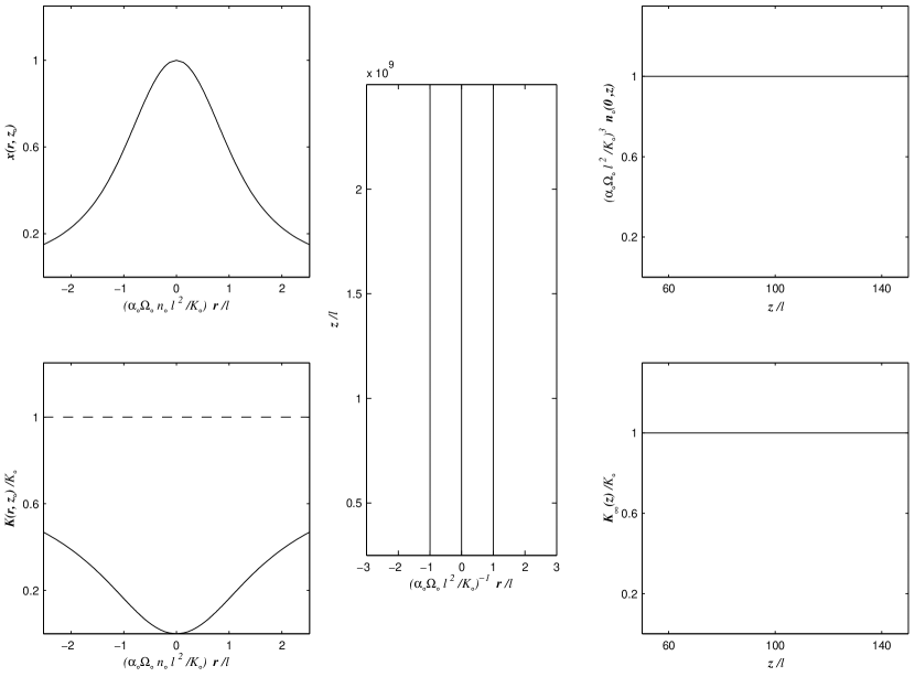
Figure 6: The behaviour of Poynting jets near the polar axis. The plots show: magnetic field structure (central frame); the normalized density at the polar axis vs. the distance along the polar axis (upper right); the total proper current integrated about the polar axis vs. the distance along the polar axis (lower right); the ratio of the density to its polar value across the polar pinch (upper left) and the integrated proper current across the polar axis (lower left). The latter two quantities are plotted for some arbitrarily chosen $z_{0}$. The central frame shows that the field lines are exact cylinders (Eq.(84)). The right panel curves use Eqs.(72) and (76). The left panel curves are obtained from Eqs.(62)–(64), (33) and (34). $K_{0}$ here is the absolute minimum of $\frac{\alpha E}{\Omega}$.

These results are illustrated in Figures 1-7. Figures 1-3 represent properties of kinetic winds as deduced from our analysis. Figure 1 illustrates the geometry of magnetic surfaces. Figures 2 and 3 represent the structure of the polar and equatorial boundary layers. Figures 4-7 represent similar properties for Poynting jets.

In all cases, the polar and null surface boundary layers which carry residual electric current may stand out observationally against the field-regions, both because of their large density contrast to them and because they possess a source of free energy that makes them potentially active by the development of instabilities. It is noteworthy that the density about the pole either does not decline with distance in the case of Poynting jets, or only very slowly (as a negative power of the logarithm of the distance) in the case of kinetic winds. It may be that what is observed as a jet be but the dense and active polar boundary layer of a flow developed on a much larger angular scale. This diffuse flow may be itself barely visible because of its very low density and activity. Null surface boundary layers, for example equatorial ones, enjoy a more favourable status than field regions from this point of view (Beskin & Okamoto, 2000), and may be observed in association with jets. The X-ray structure of the Crab Nebula (Weisskopf et al., 2000) can be understood in such a framework (Blandford, 2002). In addition, our work is relevant to the large scale aspects of pulsar winds, jets from active galaxies and gamma ray bursts (Vlahakis & Königl, 2003a, b). It is interesting to note that, from our analysis, the highest degrees of collimation are associated with flows which carry significant Poynting flux. In our next paper (Heyvaerts & Norman, 2002b), we show that such flows should actually occur, owing to the slow decline of the asymptotic proper current with distance.

Figure 1: The magnetic field structure for kinetic winds in the asymptotic field region, from Eq.(110). The functions $E(a)$ and $\Omega(a)$ have been taken as constant which implies that $q(a)=(a/A)$. On the pole $q(0)$ = 0 and at the equator $q(A)$ = 1. The field lines in each quadrant correspond to $a/A=$ $0.2$, $0.4$, $0.6$, $0.8$, $0.9$. An interpolation formula has been used to connect the asymptotic solution to a split-monopole field at the origin. The scale for $r$ and $z$ is arbitrary.

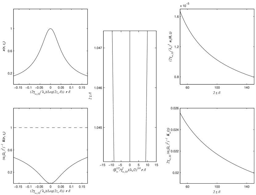
Figure 2: The behaviour of kinetic winds near the polar axis. The panels show: magnetic field structure (central frame); the normalized density (Eq.(76)) at the polar axis vs. the distance along the polar axis (upper right); the total proper current integrated about the polar axis vs. the distance along the polar axis (lower right); the ratio of the density to its polar value at the same $z$ across the polar pinch (upper left) and the integrated proper current across the polar axis (lower left). The latter two quantities are plotted for some arbitrarily chosen $z_{0}$. In the central frame, $a$ = $a_{0}\left(\frac{\lambda_{0}}{2}\right)^{3/2}$ (Eq.(115)). The slightly parabolic shape of the field lines is not clearly visible on the scale of the plot. The right panel curves are from Eqs.(72), (75) – (77) and (80) with $\lambda_{0}$ given by Eq.(78) for negligibly small $K_{\infty}$. The left panel curves are from Eqs.(62)–(64), (33), (34), (75)–(77) and (80).

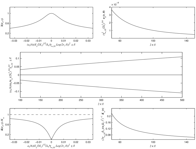
Figure 3: The behaviour of kinetic winds about the equatorial boundary layer. The panels show: the magnetic field structure (central); the normalized density $n_{e}$ = $\frac{\rho(r,0)}{\rho_{A0}}$ in the equatorial plane vs. distance along the equatorial plane (upper right); the total proper current integrated about the equatorial plane vs. distance along the equatorial plane (lower right); the ratio of the density to its equatorial value at the same $r$ across the equatorial sheet (upper right) and the integrated proper current across the equatorial sheet (lower left). The latter two quantities are plotted for some arbitrary value of $r$, $r_{0}$. For simplicity, $\Omega_{e}$, $\alpha_{e}$ and $Q_{e}$ have been set equal to $\Omega_{0}$, $\alpha_{0}$ and $Q_{0}$ respectively. The field lines (central frame, Eq.(118)) correspond to $\frac{a}{A}$ = 0.9. Their parabolic shape is not clearly visible on the scale of the plot. The plots in the right panel are from Eqs.(106) and (108), while those in the left panels are from Eqs.(99), (102), (103) and (33) with $\nu$ = $\frac{1}{2}$.

Figure 4: The magnetic field structure for Poynting jets in the field region, from Eqs.(56) and (57). From pole to equator, the contours are for $(a/A)=$ $0.4$, $0.6$, $0.7$, $0.85$, $0.9$ and $0.95$. $E(a)$ and $\Omega(a)$ are constants, while we assume, as discussed in Paper III, that $\alpha(a)=(K\Omega/(E-c^{2}))\{1+\left[((a/A)-0.8)^{2}/\sqrt{1-(a/A)}\right]\}$. The unit of the plot for the variables $r$ and $z$ is the scale $\ell$ defined in Eq.(75). An interpolation formula has been used to connect the asymptotic structure of the field to a split monopole field near the origin. Eqs.(56) and (57) become increasingly accurate with larger $r/\ell$ and $z/\ell$, the scale of the transition between the split monopole structure near the origin and the asymptotic one being arbitrary.

Figure 5: Same as figure (4). The scale in $(r/\ell)$ and $(z/\ell)$ is larger.

Figure 7: The behaviour of Poynting jets about the equatorial boundary layer. The plots show: magnetic field structure (central frame, from Eq.(118)); the normalized density $n_{e}$ = $\frac{\rho(r,0)}{\rho_{A0}}$ in the equatorial plane vs. the distance along the equatorial plane (upper right); the total proper current integrated about the equatorial plane vs. the distance along the equatorial plane (lower right); the ratio of the density to its equatorial value at the same $r$ across the equatorial sheet (upper left) and the integrated proper current across the equatorial sheet (lower left). The latter two quantities are plotted for some arbitrary value of $r$, $r_{0}$. The field structure (central frame) is plotted for $\frac{a}{A}$ = 0.9. The plots in the right panels are from Eqs.(106) and (107), while those in the left panels are from Eqs.(102), (103), (33) and (99) with $\nu$ = $\frac{1}{2}$.

References

- Appl and Camenzind (1993a) Appl, S. and Camenzind, M. 1993 A&A270, 71
- Appl and Camenzind (1993b) Appl, S. and Camenzind, M. 1993 A&A274, 699.
- Ardavan (1979) Ardavan, H. 1979, MNRAS189, 341.
- Begelman & Li (1994) Begelman, M. C. and Li, Z. Y. 1994 ApJ426, 269.
- Bell & Luçek (1995) Bell, A.R. and Luçek, S.G. 1995, MNRAS277, 1327.
- Beskin et al. (1993) Beskin, V.S., Gurevich, A.V. and Istomin, Ya. N., 1993 Physics of the pulsar magnetosphere, Cambridge University Press.
- Beskin et al. (1998) Beskin, V.S., Kuznetsova, I.V., and Rafikov, R.R. 1998 MNRAS299, 341
- Beskin & Malyshkin (2000) Beskin, V.S. and Malyshkin, L.M. 2000 Astronomy Letters 26, 208.
- Beskin & Okamoto (2000) Beskin, V.S. and Okamoto, I. 2000 MNRAS313, 445.
- Beskin & Par’ev (1993) Beskin, V.S. and Par’ev V. 1993 Uspekhi 36, 529
- Blandford (2002) Blandford, R.D. 2002, in Lighthouses of the Universe, ed. M. Gilfanov et al. (Springer:Berlin), p. 381
- Blandford & Payne (1982) Blandford, R. D. and Payne, D. G., 1982 MNRAS199, 88
- Bogovalov (1999) Bogovalov, S.V. 1999 A&A349, 1071
- Bogovalov (2001) Bogovalov, S.V. 2001 A&A371, 1155
- Bogovalov & Tsinganos (1999) Bogovalov, S. and Tsinganos, K. 1999 MNRAS305, 211.
- Bogovalov & Tsinganos (2001) Bogovalov, S. and Tsinganos, K. 2001 MNRAS325, 249
- Camenzind (1986a) Camenzind, M., 1986 A&A156, 137.
- Camenzind (1986b) Camenzind, M., 1986 A&A162, 32.
- Camenzind (1987) Camenzind, M. 1987 A&A184, 341.
- Camenzind (1989) Camenzind, M. 1989 in Accretion Disks and Magnetic Fields in Astrophysics, ed. G. Belvedere, (Dordrecht Kluwer) p 129.
- Chiueh et al. (1991) Chiueh, T. Li, Z.Y. and Begelman, M. 1991 ApJ377, 462.
- Chiueh et al. (1998) Chiueh, T. Li, Z.Y. and Begelman, M. 1998 ApJ505, 835.
- Contopoulos (1994) Contopoulos, J. 1994 ApJ432, 508.
- Contopoulos (1995) Contopoulos, J. 1995 ApJ446, 67.
- Contopoulos et al. (1999) Contopoulos, I, Kazanas, D. and Fendt, C. 1999, ApJ511, 351.
- Contopoulos & Lovelace (1994) Contopoulos, I. and Lovelace, R.V.E. 1994, ApJ429, 139.
- Fendt et al. (1993) Fendt,C., Camenzind, M. and Appl, S. 1993 A&A300, 791
- Fendt & Camenzind (1996) Fendt,C. and Camenzind, M. 1996 A&A313, 591
- Goldreich & Julian (1970) Goldreich, P. and Julian, W. H., 1970 ApJ160, 971.
- Heinemann & Olbert (1978) Heinemann, M. and Olbert, S., 1978 J. Geophys. Res.82, 23.
- Heyvaerts & Norman (1989) Heyvaerts, J. and Norman, C.A. 1989 ApJ347, 1055
- Heyvaerts & Norman (2002a) Heyvaerts, J. and Norman, C.A. 2002a ApJ, submitted
- Heyvaerts & Norman (2002b) Heyvaerts, J. and Norman, C.A. 2002b ApJ, submitted
- Koide et al. (1999) Koide, S. Shibata, K. and Kudoh, T. 1999 ApJ522, 727
- Koide et al. (2000) Koide, S., Meier, D.L., Shibata, K. and Kudoh, T. 2000 ApJ536, 668
- Koide et al. (2002) Koide, S., Shibata, K., Kudoh, T. & Meier, D.L. 2002, Science, 295, 1688
- Krasnopolsky et al. (1999) Krasnopolsky, R., Li, Z.Y., and Blandford, R. 1999 ApJ526, 631.
- Kudoh et al. (1998) Kudoh, T., Matsumoto, R., Shibata, K. 1998 ApJ508, 186.
- Li (1993a) Li, Z.Y. 1993, PhD Thesis, University of Colorado, Boulder.
- Li (1993b) Li, Z. Y. 1993 ApJ415, 118
- Li et al. (1992) Li Z. Y., Chiueh, T. and Begelman, M. 1992 ApJ394, 459.
- Lovelace (1976) Lovelace, R.V.E. 1976 Nature 262, 649
- Lovelace et al. (1987) Lovelace, R.V.E, Wang, J.C.L & Sultanen, M.E. 1987 ApJ315, L504
- Lovelace et al. (1991) Lovelace, R.V.E, Berk, H.L. and Contopolos, J. 1991 ApJ379, 696.
- Lovelace et al. (1993) Lovelace, R.V.E. Romanova, M. and Contopolos, J. 1993 ApJ403, 158.
- Luçek & Bell (1997) Luçek, S.G. and Bell, A.R. 1997 MNRAS290, 327
- Matsumoto et al. (1996) Matsumoto, R., Uchida, Y., Hirose, S., Shibata, K., Hayashi, M.R., Ferrari, A., Bodo, G & Norman, C.A. 1996 ApJ461, 115
- Michel (1969) Michel, F.C. 1969 ApJ158, 727.
- Mobarry & Lovelace (1986) Mobarry, C.M. and Lovelace, R.V.E. 1986, ApJ309, 455.
- Nishikawa et al. (1997) Nishikawa, K-I, Koide, S., Sakai, J-I, Christodoulou, D.M., Sol, H. and Mutel, R. 1997 ApJ483, L45
- Nitta (1995) Nitta, S-Y 1995 MNRAS276, 825.
- Nitta (1997) Nitta, S-Y 1997 MNRAS284, 899.
- Nitta et al. (1991) Nitta, S-Y., Takahashi, M. and Tomimatsu, A. 1991 Phys. Rev. D, 44, 2295.
- Okamoto (1975) Okamoto, I., 1975 MNRAS173, 357.
- Okamoto (1999) Okamoto, I., 1999 MNRAS307 253
- Okamoto (2000) Okamoto, I., 2000 MNRAS318 250
- Okamoto (2001) Okamoto, I., 2001 MNRAS327, 55
- Spruit et al. (1997) Spruit, H.C., Foglizzo, T. and Stehle, R. 1997 MNRAS288, 333.
- Takahashi et al. (1990) Takahashi, M., Nitta, S., Tatematsu, Y. and Tomimatsu, A. 1990 ApJ363, 206.
- Tomimatsu (1994) Tomimatsu, A. 1994 PASJ46, 123.
- Tomimatsu & Takahashi (2003) Tomimatsu, A. & Takahashi, M. 2003 ApJ592 321
- Tsinganos & Bogovalov (1999) Tsinganos, K. and Bogovalov, S. 1999 MNRAS305, 211.
- Ustyugova et al. (2000) Ustyugova G. V., Lovelace, R. V. E., Romanova, M. M., Li, H. and Colgate, S.A. 2000 ApJ541 L21
- Van Putten (1997) Van Putten, M.H.P.M. 1997 ApJ488, 69L.
- Vlahakis & Königl (2003a) Vlahakis, N. & Königl, A. 2003, astro-ph/0303482
- Vlahakis & Königl (2003b) Vlahakis, N. & Königl, A. 2003, astro-ph/0303483
- Weisskopf et al. (2000) Weisskopf, M.C., Hester, J.J., Tennant A.A., Elsner, R.F., Schulz, N.S., Marshall, H.L., Karovska, M., Nichols, J.S., Swartz, D.A., Kolodziejczak, J.J. and O’Dell, S.L. 2000 ApJ536, L81