Can Non-Gaussian Cosmological Models Explain the WMAP’s High Optical Depth for Reionization?

Abstract

The first-year Wilkinson Microwave Anisotropy Probe data suggest a high optical depth for Thomson scattering of 0.17 $\pm$ 0.04, implying that the universe was reionized at an early epoch, $z\sim 20$. Such early reionization is likely to be caused by UV photons from first stars, but it appears that the observed high optical depth can be reconciled within the standard structure formation model only if star-formation in the early universe was extremely efficient. With normal star-formation efficiencies, cosmological models with non-Gaussian density fluctuations may circumvent this conflict as high density peaks collapse at an earlier epoch than in models with Gaussian fluctuations. We study cosmic reionization in non-Gaussian models and explore to what extent, within available constraints, non-Gaussianities affect the reionization history. For mild non-Gaussian fluctuations at redshifts of 30 to 50, the increase in optical depth remains at a level of a few percent and appears unlikely to aid significantly in explaining the measured high optical depth. On the other hand, within available observational constraints, increasing the non-Gaussian nature of density fluctuations can easily reproduce the optical depth and may remain viable in underlying models of non-Gaussianity with a scale-dependence.

1 Introduction

The excess large scale polarization signal in the Wilkinson Microwave Anisotropy Probe (WMAP) data has allowed the first measurement of the optical depth to re-scattering by electrons with a value of $\tau=0.17\pm 0.04$ (Kogut et al. 2003). If interpreted as a sharp transition to a reionized universe from a neutral one, the redshift at which this transition happens is $z_{r}=17\pm 5$ (?; ?). Theoretical studies based on Cold Dark Matter (CDM) models suggest that such a high reionization redshift — beyond what was previously suggested with Gunn-Peterson troughs in $z\sim 6$ quasars from the Sloan survey (e.g., Fan et al. 2002) — generally requires significant star-formation early on, at $z>10$ (Cen 2003; Haiman & Holder 2003; Sokasian et al. 2003; Yoshida et al. 2003).

While conventional models of reionization based on ordinary stellar populations (Population II stars) formed in galaxies alone are still consistent with the measured optical depth (Chiu, Fan & Ostriker 2003; Somerville & Livio 2003), these models are not capable of explaining the high end of the allowed range for the optical depth. The best fit value of $\tau=0.17$ is only achieved in models where reionization takes place with the maximal efficiency in terms of star-formation and associated ionizing photon production (Fukugita & Kawasaki 2003; Haiman & Holder 2003; Cen 2003; Sokasian et al. 2003; Wyithe & Loeb 2003). Alternatively, with a combination of a high photon escape fraction and a top-heavy IMF in early galaxies, the resulting total optical depth can be increased to be marginally consistent with the WMAP data (e.g., Ciardi, Ferrara & White 2003). Although recent theoretical studies consistently indicate that the first stars formed out of a chemically pristine gas were rather massive (Abel, Bryan & Norman 2002; Bromm, Coppi & Larson 2002), hence supporting at least the latter condition, it is unclear whether such conditions are realized in primeval galaxies over a sufficiently long period. It is therefore intriguing to consider alternative mechanisms that do not require considerably high efficiency in star-formation or in ionizing photon production rate. Interestingly, such a scenario is possible even within the standard cosmological models. For example, as we show later in the present paper, with $\sigma_{8}$ equal to or larger than unity, the optical depth to reionization can reach within the range of the WMAP result since with a higher normalization, halos collapse slightly at earlier times and are more numerous at a given epoch when compared to models with a lower value for the normalization of the matter power spectrum.

In light of this, with currently favored values for cosmological parameters, invoking non-Gaussianities in primordial density fluctuations may be an interesting possibility and deserves further study. In the non-Gaussian models, one finds an increased fraction of high density peaks relative to Gaussian models, and these peaks are expected to collapse earlier than in the standard case (Peebles 1997; White 1998; Koyama, Soda & Taruya 1999; Robinson & Baker 2000; Willick 2000; Seto 2001; Mathis 2002). If star-formation is triggered in these collapsed halos, photons emitted from them may be able to, at least partially, reionize the universe very early on, causing a large total Thomson optical depth.

Excess non-Gaussian fluctuations generally lead to formation of structures at late times and could overproduce the cluster abundance at low redshifts (Willick 2000). However, the constraint obtained from cluster abundance is rather uncertain, and previous studies based on models of primordial non-Gaussianities (e.g., Verde et al. 2001) suggest that, in certain models where non-Gaussianities are associated with the density field, even a small primordial non-Gaussianity can significantly affect the number counts of objects at high redshifts. Avelino & Liddle (2003) recently studied the evolution of the mass fraction in collapsed halos in non-Gaussian models and calculated a simple lower estimate for the redshift of reionization.

In this Letter, we use a detailed model for the mass function in non-Gaussian models and compute the reionization history for some cases. To this end we compute the total Thomson optical depth as a function of redshift. We conclude that such non-Gaussian models, consistent with current constraints, can easily explain WMAP’s results. We also argue that, while these models may eventually be constrained with large scale structure observations, there is still some freedom to obtain the necessary non-Gaussianity with models which are strongly scale-dependent.

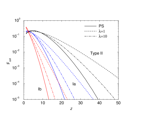
Figure 1: The fraction of mass in collapsed halos, between various mass limits (see Section 2 for a summary), as a function of redshift for the standard Press-Schechter mass function and for the non-Gaussian mass function that includes a free parameter $\lambda$ that accounts for the departure from Gaussianity. Small values for $\lambda$ represent a significant non-Gaussianity while $\lambda>100$ is consistent with Gaussian fluctuations in the density field.

2 Calculational Method

Following Haiman & Holder (2003) (hereafter HH), we study star formation and reionization using a simple toy model. Throughout the paper we assume the best fit flat $\Lambda$CDM model with power law fluctuations for the WMAP data: $(\Omega_{m},\Omega_{\Lambda},\Omega_{b},h,\sigma_{8},n_{s})=(0.27,0.73,0.044,0.72,0.9,0.99)$. Given these cosmological parameters, we calculate the collapsed fraction of baryons using a spherical halo model. HH distinguished three different types of halos based essentially on the halo mass, which captures different nature of stars formed in them. The collapsed halo fractions for each halo type is

$$F_{\rm coll}=\frac{1}{\bar{\rho}}\int_{m_{l}}^{m_{h}}dm\;mn(m,z)\,,$$ (1)

where $m_{l}$ and $m_{h}$ take values based on the gas temperature within the halo such that

$$m(z) = 0.94\times 10^{8}M_{\sun}\left(\frac{h}{0.7}\right)^{-1}\left(\frac{\Omega_{m}}{0.3}\right)^{-1/2}$$ (2)

$$\quad\times\left(\frac{1+z}{10}\right)^{-3/2}\left(\frac{\mu}{0.6}\right)^{-3/2}\left(\frac{T}{10^{4}K}\right)^{3/2}\,,$$

where $\mu$ is the mean molecular weight: in the case of ionized gas with $T\geq 10^{4}$ K, $\mu=0.6$ and for neutral gas with $T<10^{4}$ K, $\mu=1.2$. The collapse fractions are divided to three halos between 100 K and 10⁴ K (called Type II where molecular Hydrogen cooling dominates), between 10⁴ K and $2\times 10^{5}$ K (Type Ia), and above $2\times 10^{5}$ K (Type Ib). In both Type I halos, the dominant cooling mechanism to form stars involves atomic hydrogen lines.

Using the collapsed mass fractions, we can now calculate the ionized HII filling factor, which is the same as the mean electron fraction $\bar{x}_{e}(z)$, by integrating for ionization produced by collapse at all higher redshifts,

$$F_{\rm HII}(z) = \rho_{\rm b}(z)\int_{\infty}^{z}dz^{\prime}\left\{\epsilon_{\rm Ib}\frac{dF_{\rm coll}^{\rm Ib}}{dz}(z^{\prime})+\left[1-F_{\rm HII}(z^{\prime})\right]\right.\times$$ (3)

$$\left.\left[\epsilon_{\rm Ia}\frac{dF_{\rm coll}^{\rm Ia}}{dz}(z^{\prime})+\epsilon_{\rm II}\frac{dF_{\rm coll}^{\rm II}}{dz}(z^{\prime})\right]\right\}{\tilde{V}}_{\rm HII}(z^{\prime},z).$$

The second term on the right hand side includes the factor $(1-F_{\rm HII})$ to allow for photo-ionization feedback, while ${\tilde{V}}_{\rm HII}(z_{\rm on},z)$ is the volume per unit mass and unit efficiency ionized by redshift $z$ by a single source that turned on at an earlier redshift of $z_{\rm on}>z$. In Eq. (3), $\epsilon_{i}\equiv N_{\gamma}f_{*}f_{\rm esc}$ represents the overall efficiency of star-formation and photon emission, where $f_{*}$ is the fraction of baryons in the halo that turns into stars, $N_{\gamma}$ the mean number of ionizing photons produced by an atom cycled through stars (averaged over initial mass function), $f_{\rm esc}$ is the fraction of these photons escape to IGM. In the following we use fiducial values of $\epsilon$ for type Ia and Ib halos as advocated by HH. We set $\epsilon_{\rm II}=0$, i.e. we do not consider star formation in “minihalos” in which the gas can cool via molecular hydrogen cooling. It is straightforward to include Type II halos in our models, but the ionization history involving them is more complicated. For our purpose – test the effect of non-Gaussianity – it is unnecessary to introduce such additional complexity. Indeed, one aim is to see if early reionization could be obtained without invoking molecular hydrogen cooling.

The evolution of the ionization front is calculated by solving the following differential equation

$$\frac{dV}{dt}=3H(z)V+\frac{\dot{N}_{\gamma}(t)}{\bar{n}_{H}}-C\bar{n}_{\rm H}\alpha_{\rm B}V\,,$$ (4)

where $\alpha_{B}=2.6\times 10^{-13}$ cm³ s^-1 is the case B recombination coefficient. Adopting a fixed value of $\alpha_{B}$ is equivalent to assuming a constant temperature of the ionized region. Strictly speaking, this is not true, and one needs consider the evolution of the thermal state of the ionized IGM. However, with atomic cooling the gas in the ionized, photo-heated regions quickly approaches this temperature, and as shown by HH this provides a good approximation. $C=\langle n_{H}^{2}\rangle/\bar{n}_{H}^{2}$ is the clumping factor, which we take to be at a constant value of 10. $H(z)$ is the expansion rate, with $H_{0}[\Omega_{m}(1+z)^{3}+\Omega_{\Lambda}]^{1/2}$, and $\dot{N}_{\gamma}(t)$ is the rate of ionizing photon emission as a function of time. We take $\dot{N}_{\gamma}(t)$ to be a constant for $t<3.1\times 10^{6}$ years with a value of 3.7 $\times$ 10⁴⁶ s^-1 per solar mass of stellar content and decrease from this constant value as $(t/3.1\times 10^{6}{\rm yr})^{-4.5}$ thereafter. We start integration at a sufficiently high redshift, and solve Eq. (3) up to $F_{\rm HII}=1$, at which point we consider reionization is completed and keep $F_{\rm HII}$ fixed at 1 for redshift below this. The optical depth is calculated by integrating the ionized volume fraction weighted by the number density such that

$$\tau(z)=1.08\int_{0}^{z}dz\;\frac{dt}{dz}c\sigma_{T}n_{\rm H}(z)F_{\rm HII}(z).$$ (5)

The factor 1.08 accounts approximately for the contribution of helium reionization (see HH).

3 Non-Gaussianity

The collapsed fraction can be calculated using a standard mass function, such as the Press-Schechter theory (PS; Press & Schechter 1974) based on Gaussian density fluctuations, or the numerical simulated mass function by Jenkins et al. (2001), which was used by HH. To describe the linear power spectrum, we use the transfer function from Eisensetin & Hu (1998). We now modify the standard mass function by adding non-Gaussian fluctuations to the density field. To compare with various available constraints, we make use of a simple model for the non-Gaussian mass function which has been previously studied in the literature (Koyama, Soda & Taruya 1999; Willick 2000), though we note that, under specific models of primordial non-Gaussianity, more detailed mass functions can be constructed (e.g., Matarrese, Verde & Jimenez 2000). We write the generalized form of the mass function as

$$n(m,z)=\frac{\bar{\rho}}{m}\frac{\delta_{c}}{\sigma^{2}(m,z)}\frac{d\sigma(m,z)}{dm}\psi\left(\frac{\delta_{c}}{\sigma(m,z)}\right)\,,$$ (6)

where the probability distribution function for density fluctuation, $\delta$, is written in terms of a dimensionless function $\psi(x)$:

$$P(\delta|\sigma)=\sigma^{-1}\psi\left(\frac{\delta_{c}}{\sigma}\right)\,,$$ (7)

where $\int\psi(x)dx=1$, $\int x\psi(x)dx=0$ and $\int x^{2}\psi(x)dx=1$. Here, $\sigma(M,z)$ is the rms mass function on a scale corresponding to a mass $m$, and $\delta_{c}$ is the critical density for collapse (see, e.g., Kitayama & Suto 1996 for details). The standard Press-Schechter formula assumes a Gaussian probability distribution function (PDF) such that $\psi(x)=2Ae^{-x^{2}/2}$ and $A=(2\pi)^{-1/2}$. To include a mild non-Gaussian tail to the Gaussian description, essentially a skewness, we consider a PDF which is based on the Poisson description, but modified appropriately for the continuous variables involved (see, Willick 2000 for details). The function is written as

$$\psi(x)=2A\frac{\lambda^{\sqrt{\lambda}x+\lambda+0.5}e^{-\lambda}}{\Gamma(\sqrt{\lambda}x+\lambda+1)}\,,$$ (8)

such that $\lambda$, which is a function of redshift, is a free-variable that captures the non-Gaussian nature of the PDF; As $\lambda$ is increased, the mass function approaches to the PS value for Gaussian distribution of density fluctuations. $A$ is chosen to return the correct normalization: $\int mn(m,z)dm=\bar{\rho}(z)$.

Note that in our non-Gaussian mass function, skewness, $S_{3}$, scales as $\lambda^{-1}$, which explains why non-Gaussianity increases with decreasing $\lambda$. In terms of the moments of the primordial density field, one can write skewness as

$$S_{3}(m,z)=\epsilon\frac{\mu_{3}(m,z)}{\sigma^{4}(m,z)}\,,$$ (9)

where $\mu_{3}$ is the third moment of the density perturbations, scaled to a redshift of $z$, when $\epsilon$ is the parameter related to the quadratic correction (Matarrese, Verde & Jimenez 2000). If we ignore for now the mass-, or equivalently scale-dependence, of primordial non-Gaussianity, then $\mu_{3}\sim 6\sigma^{4}$, and assuming linear growth of fluctuations, $S_{3}(z)\sim 6\epsilon/G(z)$ where $G(z)$ is the growth factor. The latter scaling can be understood based on the fact that $\mu_{3}(m,z)$ and $\sigma^{2}(m,z)$ scale with redshift as $G^{3}(z)$ and $G^{2}(z)$, respectively. Since in our mass function, $S_{3}\sim\lambda^{-1}$, we expect $\lambda$ to behave as $\sim(\epsilon^{-1}/6)G(z)$ as a function of redshift.

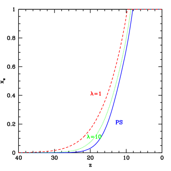
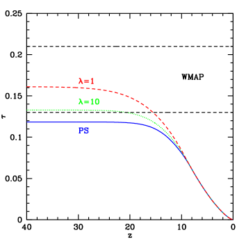
Figure 2: Left: The volume ionized fraction, $x_{e}(z)\equiv F_{\rm HII}(z)$ as a function of redshift. Middle: The Thomson optical depth for electron scattering. The models are based on “ordinary” star-formation in Type I halos only. The Press-Schechter mass function leads to an optical depth with a value of 0.097 while the non-Gaussian mass functions lead to values of 0.11 and 0.13 for $\lambda=10$ and $\lambda=1$, respectively. The two black dashed lines in the middle and right panels indicate the range of the first year WMAP result. Right: Same as the middle plot, but with $\sigma_{8}=1$ and keeping all other parameters the same.

In Fig. 1, we plot the collapsed fraction of these halos for the standard PS mass function and the non-Gaussian mass functions with $\lambda=10$ and $\lambda=1$ as a function of redshift. We note that these values could be a function of redshift, although we have taken $\lambda$ to be a constant, for purposes of the present discussion. As $\lambda$ is decreased, or models become strongly non-Gaussian, the fraction of mass in collapsed halos increases at a fixed redshift. This illustrates the basic idea behind our calculation that with increasing non-Gaussianity of the density field, there are more high overdensity peaks which collapse earlier. These early collapsing halos can form stars at an earlier time than in the standard description and reionize the universe such that the total optical depth is higher than previously estimated in the Gaussian models.

In Fig. 2, we show the ionization fraction and optical depth for the models with the PS mass function and with the non-Gaussian mass function with $\lambda=10$ and $\lambda=1$. In addition to our standard cosmological values, to illustrate the increase in the optical depth by halos collapsing at an earlier time, we also calculate the optical depth in a model where $\sigma_{8}=1$ (Fig.2, right plot). We emphasize that such high values of $\sigma_{8}$ easily make the optical depth large even within the Gaussian model.

For a given set of cosmological parameters, higher optical depths can be achieved with the non-Gaussian mass functions. As shown in Fig. 2, compared with the standard Gaussian PS function, there is only a moderate increase in optical depth for the $\lambda=10$ model (about 0.01 in $\tau$). This difference is in fact comparable in size with the difference between the PS and Jenkins mass functions: it is well known that compared with the PS mass function, the Jenkins et al. (2001) function predicts an excess of halos at the upper end of the halo mass. Our calculated optical depth with the Jenkins et al. (2001) mass function of $\sim$ 0.13 is consistent with previous calculations on the optical depth based on Pop II stars alone (e.g., HH; Fukugita & Kawasaki 2003). To increase the optical depth beyond this value, one can either add more Population III stars at earlier epochs (Cen 2003; Wythie & Loeb 2003; Sokasian et al. 2003) or, as we have considered, by considering smaller $\lambda$ value (greater non-Gaussianity) while resorting only ordinary stellar populations.

A significantly non-Gaussian model with $\lambda\sim 1$ increases the optical depth by a large fraction (about 0.04 in $\tau$). From Eq. 9 and the expected scale with redshift, such a non-Gaussianity implies a primordial non-Gaussianity with $\epsilon\sim 5\times 10^{-3}$. Non-Gaussianities at this level can soon be tested with observations of galaxy counts at redshifts of 5, though low redshift large scale structure observations will not be helpful for this purpose (Verde et al. 2001). At present, according to Willick (2000) (see his Fig. 11), for $\Omega_{m}=0.27$, the low redshift galaxy cluster abundance is consistent at the 90% confidence level with a non-Gaussian mass function of $\lambda<14$. The cluster abundance at low-redshift is not a strong discriminator of non-Gaussian models, as argued by Verde et al. (2001). Note that only a constraint on the upper limit of $\lambda$ is available from the cluster abundance in Willick (2000), though in Koyama et al. (1999; also, Robinson, Gawiser & Silk 1998) $\lambda\sim 3$ is preferred for $\Lambda$CDM cosmological models. Again this is not a strong constraint of non-Gaussianity at redshifts of order 30.

Apart from low and moderate redshifts observations, non-Gaussianity can also be constrained, at a redshift of 1100, from observations of cosmic microwave background anisotropies (e.g., Komatsu et al. 2003). Current constraints indicate a limit of 134 on $f_{\rm nl}$, at the 95% confidence level; this parameter is related to the quadratic corrections to potential field and is different from $\epsilon$ we have been using to describe primordial non-Gaussianity based on corrections to the density field directly. Through the Poisson function, one can relate the two parameters such that at large scales of order 100 Mpc, roughly, $f_{\rm nl}\sim 2\times 10^{3}\epsilon$, and the upper limit on $f_{\rm nl}$ of 134 from WMAP corresponds to $\epsilon<7\times 10^{-2}$ and allows for significant non-Gaussianity, rendering a lower limit on $\lambda$ at a redshift $\sim$ 30 of 0.08. While cluster counts from low redshifts have constrained the upper limit and CMB observations have constrained the lower limit, the allowed range is still significant enough to produce substantial non-Gaussian fluctuations and to easily reproduce the observed optical depth with early formation of structures and first stars.

Note that with completed WMAP results and with Planck, the limits on non-Gaussianity will be improved and, naively, small values for $\lambda$ at $z\sim 30$ may be ruled out. Such a limit, however, cannot fully constrain non-Gaussianities, since one might still circumvent this by considering scale-dependent non-Gaussian models. For example, one can apply the significant non-Gaussianity to scales which are related to star-formation at redshifts above 10 and still allow such non-Gaussianity to remain today. It will then affect the number counts of $\sim 10^{8}$ M_☉ halos at low redshifts, but CMB anisotropies at large scales will remain nearly Gaussian. The same models can also be tuned such that cluster counts at low redshifts remain Gaussian also. We note that it is not difficult to envision how such models can be constructed with examples including non-standard inflationary models (Wang & Kamionkowski 2000; Bartolo, Matarrese & Riotto 2002; Bernardeau & Uzan2003) and models with primordial black hole formation proposed by Bullock & Primack (1997). While constructing a concrete model for producing such scale-dependent non-Gaussian primordial fluctuations is beyond the scope of the present study, we argue that these models can also be constrained eventually. The best way to probe the level of non-Gaussianity suggested above, and at scales related to this problem, may be to study number counts of galaxies at the highest redshifts possible (Verde et al. 2001). Another possibility involves a measurement of the non-Gaussianity in the surface brightness fluctuations produced by first stars and proto-galaxies in the near-infrared background and potentially detectable with upcoming deep observations from Near-IR Imaging Camera on the ASTRO-F mission (Cooray et al. 2003). Studying these constraints on the presence of non-Gaussianities at highest redshifts related to formation of first objects is clearly needed to understand the extent to which the reionization process is affected.

4 Summary

We have examined how the observed high optical depth is achieved in cosmological models with non-Gaussian primordial density fluctuations. In these models, high over-density peaks due to the non-Gaussianity collapse early on and may harbor first stars at redshifts above what is generally expected in the standard Gaussian model. For mild non-Gaussian fluctuations at redshifts of 30, the increase in optical depth is at the level of 0.01, and it is unlikely to explain the observed value of optical depth by this mechanism alone. To obtain significant increase in the optical depth, the first collapsing halos associated with the primordial non-Gaussianity must contribute to reionization significantly. A substantial volume fraction of the IGM may be reionized if a number of Population III stars are formed in these early halos. We found that increasing the degree of non-Gaussianities can easily reproduce the high optical depth. Such models are still viable within constraints from both cluster number counts at low redshifts and CMB anisotropies at a redshift of 1100. While constraints from these two redshift ends will improve, models with scale-dependent non-Gaussianity are possible to explain the optical depth. Such models will only be constrained by probes of non-Gaussianity related to mass scales of 10⁸ M_sun at redshifts of 30 and will involve, for example, study of first galaxy counts at very high redshifts.

The ongoing operation of WMAP will pin down a presice value for the total optical depth. For a longer-term, post-WMAP CMB polarazation experiments such as Planck will probe the reionization history (Kaplinghat et al. 2003), and detection of the second-order polarization anisotropies can place additional constraints on details of the reionization process (Liu et al. 2001). Data from these future observations will improve our picture of reionization and will enable us to further distinguish theoretical models related to the first generation of luminous structure formation.

References

- [Abel, Byran & Norman ¡2002¿] Abel, T., Bryan, G.L., & Norman, M.L., 2002, Science, 295, 93
- [Bartolo, Matarrese, Riotto ¡2002¿] Bartolo, N., Matarrese, S., Riotto, A., 2002, Physical Review D 65, 103505
- [Bernardau, Uzan ¡2003¿] Bernardeau, F. & Uzan, J.P., 2003, Physical Review D 67, 121301
- [Bromm, Coppi & Larson ¡2002¿] Bromm, V., Coppi, P.S., & Larson, R.B., 2002, ApJ, 564, 23
- [Bullock & Primack ¡1997¿] Bullock, J. S. & Primack, J. R., 1997, PRD, 55, 7423
- [Cen ¡2003¿] Cen, R., 2003, ApJ, 591, 12
- [Ciardi et al. ¡2003¿] Ciardi, B., Ferrara, A., White, S.D.M., 2003, submitted to MNRAS
- [Cooray et al ¡2003¿] Cooray, A., Bock, J. J., Keating, B., Lange, A. & Matsumoto, T. 2003, ApJ submitted, astro-ph/0308407
- [Eisenstein, Hu ¡1998¿] Eisenstein, D. & Hu, W, 1998, ApJ, 496, 605
- [Fan et al ¡2002¿] Fan, X., Narayanan, V. K., Strauss, M. A., White, R. L., Becker, R. H.., Pentericci, L. & Rix, H. 2002, AJ, 123, 1247
- [Fukugita & Kawasaki ¡2003¿] Fukugita, M. & Kawasaki, M. 2003, MNRAS, 343, L25
- [Haiman, Abel & Madau ¡2001¿] Haiman, Z., Abel, T., & Madau, P. 2001, ApJ, 551, 559
- [Jenkins et al. ¡2001¿] Jenkins, A., Frenck, C. S., White, S. D. M., et al. 2001, MNRAS, 321, 372
- [Kaplinghat ¡2003¿] Kaplinghat, M., Chu, M., Haiman, Z., Holder, G. P., Knox, L., 2003, ApJ, 583, 24
- [Kitayama & Suto ¡1996¿] Kitayama, T. & Suto, Y. 1996, ApJ, 480, 493
- [Komatsu et al ¡2003¿] Komatsu, E., et al, 2003, ApJS, 148, 119
- [Kogut et al ¡2003¿] Kogut, A., et al, 2003, ApJS, 148, 161
- [Liu et al ¡2001¿] Liu, G.-C., Sugiyama, N., Benson, A. J., Lacey, C. G., Nusser, A., 2001, ApJ, 504, 516
- [Mathis ¡2002¿] Mathis, H. 2002, PhD thesis, University of Toulouse
- [Matarrese, Verde & Jimenez ¡2000¿] Matarrese, S., Verde, L. & Jimenez, R. 2000, ApJ, 541, 10
- [Koyama et al ¡1999¿] Koyama, K., Soda, J. & Taruya, A. 1999, MNRAS, 310, 1111
- [Peebles ¡1997¿] Peebles, P. J. E. 1997, ApJ, 483, L1
- [Press & Schechter ¡1974¿] Press, W. H., Schechter, P. 1974, ApJ, 187, 425 [PS]
- [Robinson & Baker ¡2000¿] Robinson, J. & Baker, J. 2000, MNRAS. 311, 781
- [Robinson et al. ¡2000¿] Robinson, J., Gawiser, E., & Silk, J. 2000, ApJ. 532, 1
- [Seto ¡2001¿] Seto, N., 2001, ApJ, 553, 488
- [Shapiro & Giroux ¡1987¿] Shapiro, P. R. & Giroux, M. N., 1987, ApJL, 321, 107
- [Sokasian et al. ¡2003¿] Sokasian, A., Yoshida, N., Abel, T., Hernquist, L. Springel, V. 2003, astro-ph/0307451
- [Somerville & Livio ¡2003¿] Somerville, R. S. & Livio, M. 2003, astro-ph/0303017
- [Spergel et al ¡2003¿] Spergel, D.N., et al, 2003, ApJS, 175
- [Wang & Kamionkowski ¡2000¿] Wang, L. & Kamionkowski, M., 2000, PRD 61, 063504
- [Willick ¡2000¿] Willick, J. 2000, ApJ, 530, 80
- [Wyithe & Loeb ¡2003¿] Wyithe, S., & Loeb, A., 2003, ApJL, 586, 693
- [Verde et al ¡2000¿] Verde, L., Jimenez, R., Kamionkowski, M., & Matarrese, S. 2001, MNRAS, 325, 412
- [Yoshida et al. ¡2003¿] Yoshida, N., Abel, T., Hernquist, L., & Sugiyama, N., 2003, ApJ, 592, 645