Abstract

Neutrino-driven winds are thought to accompany the Kelvin-Helmholtz cooling phase of nascent protoneutron stars in the first seconds after a core-collapse supernova. These outflows are a likely candidate as the astrophysical site for rapid neutron-capture nucleosynthesis (the $r$-process). In this chapter we review the physics of protoneutron star winds and assess their potential as a site for the production of the heavy $r$-process nuclides.

We show that spherical transonic protoneutron star winds do not produce robust $r$-process nucleosynthesis for ‘canonical’ neutron stars with gravitational masses of 1.4 M_⊙ and coordinate radii of 10 km. We further speculate on and review some aspects of neutrino-driven winds from protoneutron stars with strong magnetic fields.

Protoneutron Star Winds

1 Introduction

1.1 $r$-Process Nucleosynthesis

A complete and self-consistent theory of the origin of the elements has been the grand program of nuclear astrophysics since the field’s inception. Of the several distinct nuclear processes which combine to produce the myriad of stable nuclei and isotopes we observe, none has generated more speculation than $r$-process nucleosynthesis (Wallerstein 1997). The $r$-process, or rapid neutron-capture process, originally identified in Burbidge et al. (1957) and Cameron (1957), is a mechanism for nucleosynthesis by which seed nuclei capture neutrons on timescales much shorter than those for $\beta^{-}$ decay. The rapid interaction of neutrons with heavy, neutron-rich, seed nuclei allows a neutron capture-disintegration equilibrium to establish itself among the isotopes of each element. The nuclear flow proceeds well to the neutron-rich side of the valley of $\beta$-stability and for sufficient neutron-to-seed ratio ($\mathrel{\hbox{\hbox to0.0pt{\hbox{\lower 5.0pt\hbox{$\sim$}}\hss}\hbox{$>$}}}$100) the $r$-process generates the heaviest nuclei (e.g., Eu, Dy, Th, and U), forming characteristic abundance peaks at $A\sim 80$, 130, and 195 (e.g. Burbidge et al. 1957; Meyer & Brown 1997; Wallerstein et al. 1997).

The neutron-to-seed ratio is the critical parameter in determining if $r$-process nucleosynthesis succeeds in producing nuclei up to and beyond the third abundance peak. If the neutron-to-seed ratio is too small, the $r$-process may only nuclei up to the first or second abundance peak. In a given hydrodynamical flow, the neutron-to-seed ratio is set primarily by the entropy ($s_{\rm a}$; ‘a’ here stands for ‘asymptotic’) of the flow, the neutron richness of the matter, and the dynamical timescale for expansion. The neutron richness is generally quantified by the the electron fraction ($Y_{e}^{\rm a}$, the number density of electrons per baryon). The dynamical timescale ($\tau_{\rm dyn}$) is a characteristic time for expansion, i.e. the $e$-folding time for temperature or density at a given temperature. Thus, $s_{\rm a}$, $Y^{\rm a}_{e}$, and $\tau_{\rm dyn}$ set the neutron-to-seed ratio. The higher the entropy, the lower the electron fraction, and the shorter the dynamical timescale, the larger the neutron-to-seed ratio and the higher in $A$ the nucleosynthetic flow will proceed (e.g. Hoffman, Woosley, & Qian 1997; Meyer & Brown 1997).

1.2 Observational Motivation: A Remarkable Concordance

Recent observations of neutron-capture elements in ultra-metal-poor ([Fe/H]$\mathrel{\hbox{\hbox to0.0pt{\hbox{\lower 4.0pt\hbox{$\sim$}}\hss}\hbox{$<$}}}-2.5$] halo stars (Sneden et al. 1996; Burris et al. 2000; McWilliam et al. 1995a,b; Cowan et al. 1996; Westin et al. 2000; Hill et al. 2001) show remarkable agreement with the scaled solar $r$-process abundance pattern for $A\mathrel{\hbox{\hbox to0.0pt{\hbox{\lower 5.0pt\hbox{$\sim$}}\hss}\hbox{$>$}}}135$. Particularly for atomic numbers between $N=55$ and $N=75$, the distribution of abundances in these halo stars is identical with solar. Prototypical of this class are the stars CS 22892-052, BD +17^o3248 and HD 115444 (Cowan & Sneden 2002). Figure 1 shows the scaled solar $r$-process abundances (solid line) together with those from the ultra-metal-poor halo star CS 22892-052 (points with error bars) as a function of atomic number. Note both the tight correspondence between the sun and CS 22892-052 above the second $r$-process peak and the large discrepancies at lower atomic number, in particular the elements Sn, Ag, and Y. The fact that a class of very old halo stars share the same relative abundance of $r$-process elements above the second peak suggests a universal mechanism for producing these nuclei, which must act early in the chemical enrichment history of the galaxy.

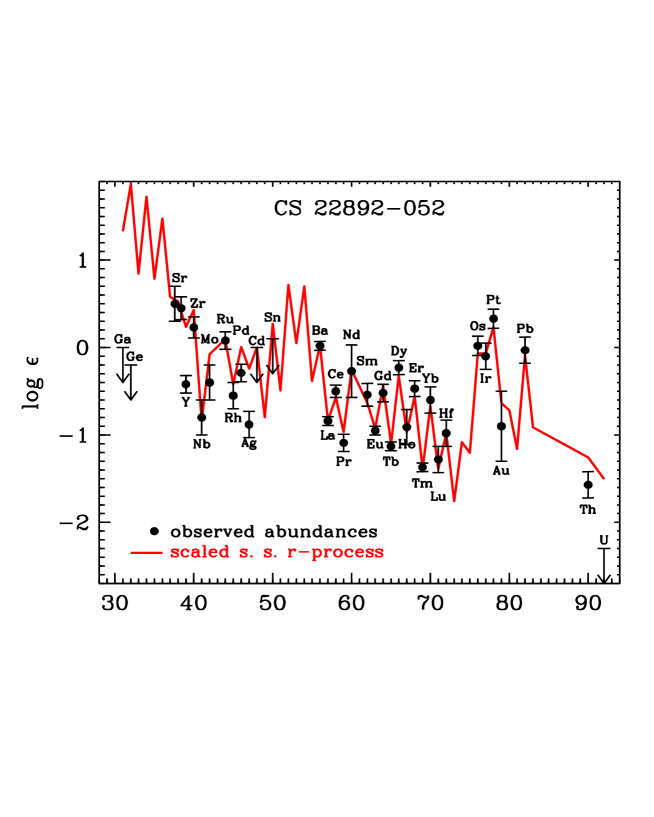
Figure 1: The scaled solar $r$-process abundances (solid line) and the abundances from CS 22892-052 (dots with error bars) as a function of atomic number (Chris Sneden, private communication).

The fact that observations of ultra-metal-poor halo stars show significant and scattered deviations from the scaled solar $r$-process abundance pattern below $A\sim 130$ has implied that there are perhaps two or more $r$-process sites (Qian, Vogel, & Wasserburg 1998; Wasserburg & Qian 2000; Qian & Wasserburg 2000). In these models of $r$-process enrichment, distinct astrophysical sites account for the observed $r$-process abundances below and above $A\sim 130$. Important in these considerations are the constraints set on the site or sites of the $r$-process by the integrated galactic $r$-process budget. For example, if all supernovae produce neutron stars that are accompanied by protoneutron star winds that produce a robust $r$-process, then, given a supernova rate of one every 50-100 years, 10${}^{-5}-$10^-6 M_⊙ of $r$-process material must be injected into the interstellar medium per event (Qian 2000). These numbers are to be contrasted with those from any other potential $r$-process site. For example, if the material possibly ejected to infinity in the formation of a black hole from neutron-star/neutron-star mergers accounts for the total galactic $r$-process budget (Freiburghaus, Rosswog, & Thielemann 1999, and references therein; Rosswog et al. 1999), then 10${}^{-1}-$10^-2 M_⊙ of $r$-process material must be ejected per event, given an event rate of one every 10⁵ years (Kalogera et al. 2001; Qian 2000 and references therein).

Because the total $r$-process budget of the galaxy is fairly well known, any potential site must do more than just match the entropy, electron fraction, and dynamical timescales required for a high neutron-to-seed ratio. Simply attaining the necessary physical conditions for a neutron-to-seed ratio above $\sim$100 is not sufficient. The astrophysical site, given an event rate, must be able to consistently produce the robust $r$-process abundance pattern in ultra-metal-poor halo stars in accordance with the total galactic $r$-process budget. Thus, if $M_{\rm ej}^{\rm r}$ is the total mass of $r$-process material produced per event, the process of assessing an astrophysical site’s potential for the $r$-process is merely a matter of mapping the region in $s_{\rm a}-Y_{e}^{\rm a}-\tau_{\rm dyn}-M_{\rm ej}^{\rm r}$ space physically accessible to the potential site. In what follows here we review the results for just-post-supernova, neutrino-driven protoneutron star winds.

1.3 Protoneutron Star Winds

The successful two-dimensional supernova explosion obtained by Burrows, Hayes, & Fryxell (1995) shows clearly a post-explosion neutrino-driven wind emerging into the evacuated region above the newly formed protoneutron star and behind the rapidly expanding supernova shock. Although no study was made of this outflow as a function of progenitor, such a wind phase might naturally accompany the post-explosion cooling epoch in many core-collapse supernovae.

A multiple of $10^{53}$ erg of binding energy will be lost as the nascent neutron star cools and contracts over its Kelvin-Helmholtz cooling time ($\sim 10-20$ seconds). This energy will be carried away predominantly by all species of neutrino. A small fraction of that energy will be deposited in the surface layers of the protoneutron star, ablating material from its upper atmosphere and driving a hydrodynamical wind. Whether this wind succeeds in escaping to infinity, or is prevented by fallback and reverse shocks as the supernova shock encounters the density stratifications of the overlying stellar mantle is an important future area of study. In addition, the actual emergence of the wind - how it overcomes the non-zero pressure of the matter exterior to the protoneutron star - has not been fully explored. In this work, however, we assume the existence of such outflows as evidenced by the calculation of Burrows, Hayes, & Fryxell (1995) as well as those of Janka & Müller (1995), and Takahashi, Witti, & Janka (1994). Our goal is to explore the basic physics of neutrino-driven outflows and assess this site as a candidate for $r$-process nucleosynthesis.

The basic scenario is as follows: as the supernova shock propagates outward in a successful explosion, the pressure in the region between the protoneutron star and the shock decreases and the wind, powered by neutrino heating, emerges into the post-shock ejecta. The surface of the protoneutron star is hot (temperatures of $\sim 5$ MeV) and has a low electron fraction (typically, $Y_{e}\sim 0.1$). The matter there is composed of relativistic charged leptons, free nucleons, and trapped photons. As the wind is driven outward, the matter descends a gradient in density and temperature. The wind material is heated only within the first $\sim$50 km, primarily via the charged-current absorption processes on free nucleons $\nu_{e}n\rightarrow pe^{-}$ and $\bar{\nu}_{e}p\rightarrow ne^{+}$, and its entropy increases concomitantly. As the temperature of the matter drops below $\sim 1$ MeV, nucleons combine into alpha particles, neutrino heating ceases and the material expands adiabatically with entropy $s_{\rm a}$. These charged-current processes also set the asymptotic electron fraction. As the matter expands away from the protoneutron star surface and the chemical equilibrium between $\nu_{e}$ and $\bar{\nu}_{e}$ neutrinos obtained near the neutrino decoupling radius (the neutrinosphere) is broken, the luminosity and energy density of the electron-type neutrino species determine the electron fraction. Typically, within 10 km of the protoneutron star surface $Y_{e}$ asymptotes to $Y_{e}^{\rm a}$. At a temperature of $\sim$0.5 MeV (a radius in most models of $\sim$100 km) alpha particles combine with the remaining free neutrons in an $\alpha$-process to form seed nuclei (Woosley & Hoffman 1992). At this location in the temperature profile, it is the steepness of the density or temperature gradient that sets the dynamical timescale of the wind. Simply stated, short dynamical timescales are favored for the $r$-process because for faster expansions there is less time to build seed nuclei, and, hence, the neutron-to-seed ratio is preferentially larger, all else being equal. When the wind material finally reaches a temperature of $\sim$0.1 MeV (at a radius of several hundred kilometers) the $r$-process may begin if the neutron-to-seed ratio, as set by $Y_{e}^{\rm a}$, $s_{\rm a}$, and $\tau_{\rm dyn}$, is sufficiently high.

Because the success of the $r$-process is so dependent on the neutron-to-seed ratio and, hence, the electron fraction, entropy, and dynamical timescale of the nucleosynthetic environment, we focus on these quantities and their sensitivity to various parameters of the protoneutron star. In addition to establishing correlations between these quantities in neutrino-driven wind environments, we must also fold in the constraint on the total mass ejected. We will show in §4 that this constraint on $M_{\rm ej}^{\rm r}$ significantly limits the $s_{\rm a}-Y_{e}^{\rm a}-\tau_{\rm dyn}$ space of relevance for winds.

1.4 Previous Work

Duncan, Shapiro, & Wasserman (1986) were the first to explore the physics of neutrino-driven winds. They identified a number of important scaling relations and the basic systematics and dependencies of the problem. In addition, they explored the relative importance of the neutrino and photon luminosities in determining the resulting hydrodynamics. Recent investigations have focused on the potential of these outflows for $r$-process nucleosynthesis as suggested in Woosley & Hoffman (1992). Witti, Janka, & Takahashi (1994) and Takahashi, Witti, & Janka (1994) showed that although interesting $\alpha$-process nuclei were created in their models of protoneutron star winds, conditions for a successful $r$-process fell short in entropy by a factor of $\sim 5$. Qian & Woosley (1996) made analytical estimates of the fundamental wind properties and systematics and compared their scalings to numbers from hydrodynamical simulations. They further explored interesting variations to their models such as inserting artificial heating sources and applying an external boundary pressure. These results were followed by nucleosynthetic calculations, taking wind trajectories as the time-history of Lagrangean mass elements in Hoffman, Woosley, & Qian (1997). These efforts also showed that with reasonable variations in the input physics protoneutron star winds do not achieve high enough entropy for the dynamical timescales and electron fractions derived.

Cardall & Fuller (1997) extended the analytical work of Qian & Woosley (1996) to general-relativistic flows. They found that significant enhancements in entropy might be obtained from compact neutron stars with large $M/R$. Several general-relativistic treatments of the problem followed, including the work of Otsuki et al. (2000), Sumiyoshi et al. (2000), Wanajo et al. (2001), and Thompson, Burrows, & Meyer (2001). In the last of these, purely transonic steady-state wind solutions were derived in general relativity, with a simultaneous solution for the evolution of the electron fraction in radius and a careful treatment of the boundary conditions.

Note that we distinguish here between models of protoneutron star winds and bubbles. The former is typified by those works already discussed, in which the wind velocity approaches the local speed of sound, or a large fraction of the speed of sound somewhere in the flow. Such winds were realized in the self-consistent supernova calculations in Burrows, Hayes, & Fryxell (1995). In contrast, in the work of Woosley et al. (1994) the protoneutron star outflow reached speeds of only a very small fraction of the sound speed in the region between the protoneutron star and the expanding supernova shock. Approximately 18 seconds after collapse and explosion, Woosley et al. (1994) obtained entropies of $\sim$400 (throughout, we quote entropy in units of k_B per baryon), long dynamical timescales, and electron fraction ($Y_{e}$) in the range $0.36-0.44$. However, in their model the supernova shock reached only 50,000 km at these late times. In turn, this external boundary caused the wind material to move slowly. It remained in the heating region for an extended period, thus raising the entropy above what any simulation or analytical calculation has since obtained. Although the $r$-process proceeded to the third abundance peak in their calculation, nuclei in the mass range near $A\sim 90$ (particularly, ⁸⁸Sr, ⁸⁹Y, and ⁹⁰Zr) were overproduced by more than a factor of 100.

1.5 This Review

In §2, we review the fundamental and general equations for time-independent energy-deposition-driven winds in Newtonian gravity and in general relativity. We also discuss the integrals of the flow and our numerical procedure for solving the relevant equations. In §3 we discuss some of the particulars of modeling protoneutron star winds, including the neutrino heating function, the equation of state, and the evolution of the electron fraction. We further critically examine several of the underlying assumptions that must accompany any such model. §4 summarizes our results for spherical winds. In §5 we consider the possible effects of magnetic fields and speculate on a number of issues in need of more thorough investigation. In §6 we summarize and conclude.

2 Hydrodynamics

2.1 The Newtonian Wind Equations

Assuming time-independent wind solutions, the equation for mass conservation is simply

$${\bf\nabla\,\,\cdot}\,\,(\rho{\bf v})=0,$$ (1)

implying that the mass-outflow rate ($\dot{M}$) of a wind is a constant in radius. In spherical symmetry, $\dot{M}=4\pi r^{2}\rho v={\rm constant}$. This expression yields a differential equation for the evolution of the matter velocity in radius,

$$\frac{1}{v}\frac{dv}{dr}=-\frac{1}{\rho}\frac{d\rho}{dr}-\frac{2}{r}.$$ (2)

The equation for momentum conservation, neglecting the mass of the wind itself, is simply

$$v\frac{dv}{dr}=-\frac{1}{\rho}\frac{dP}{dr}-\frac{GM}{r^{2}}+F_{\nu},$$ (3)

where $M$ is the total mass of the protoneutron star. Although we include it here for completeness, the radiation force due to the neutrinos ($F_{\nu}$) can be safely neglected. This approximation is justified because the neutrino Eddington luminosity ($L_{\nu}^{\rm Edd}=4\pi GMc/\kappa_{\nu}$) is much larger than the neutrino luminosities that accompany the protoneutron star cooling/wind evolutionary phase. $\kappa_{\nu}$ is the total neutrino opacity and is dominated by $\nu_{e}n\rightarrow pe^{-}$ and $\bar{\nu}_{e}p\rightarrow ne^{+}$ for the electron and anti-electron neutrino, respectively. The $\mu$- and $\tau$-neutrino opacity is dominated by neutral-current scattering off free nucleons, the wind heating region being unpopulated by nuclei. Including these processes, one finds that $L_{\nu}^{\rm Edd}\mathrel{\hbox{\hbox to0.0pt{\hbox{\lower 5.0pt\hbox{$\sim$}}\hss}\hbox{$>$}}}10^{55}$ erg s^-1. We are thus safe in taking $F_{\nu}=0$ because we consider winds with only $L^{\rm tot}_{\nu}<5\times 10^{52}$ erg s^-1.

Because neutrinos contribute heating and cooling to the flow, we must couple to these equations to the first law of thermodynamics. We define the net specific heating rate, $\dot{q}={\rm Heating}-{\rm Cooling}$, so that

$$\frac{d\epsilon}{dt}=\dot{q}=T\frac{ds}{dt}+\frac{P}{\rho^{2}}\frac{d\rho}{dt},$$ (4)

where $d/dt=[\partial/\partial t+v\cdot\nabla]$. In the steady state, $\partial/\partial t=0$ and we obtain

$$\dot{q}=Tv\frac{ds}{dr}=C_{V}v\frac{dT}{dr}-\frac{vT}{\rho^{2}}\left.\frac{\partial P}{\partial T}\right|_{\rho}\frac{d\rho}{dr}.$$ (5)

We choose to reduce eqs. (2), (3), and (5) to a set of coupled differential equations for $dv/dr$, $d\rho/dr$, and $dT/dr$ that make the physics of the wind solution manifest and the solution to the problem more easily obtained. We start by eliminating the pressure. Expanding $P$ differentially in $\rho$ and $T$, we have that

$$dP=\left.\frac{\partial P}{\partial\rho}\right|_{T}\,\delta\rho+\left.\frac{\partial P}{\partial T}\right|_{\rho}\,\delta T.$$ (6)

Defining ($D$) as

$$D=\frac{T}{\rho}\left.\frac{\partial P}{\partial T}\right|_{\rho},$$ (7)

we obtain

$$c_{s}^{2}=c_{T}^{2}+\frac{D^{2}}{C_{V}\,T}.$$ (8)

where $C_{V}$ is the specific heat at constant volume, $c_{s}(=\left.\partial P/\partial\rho\right|_{s}$) is the adiabatic sound speed, and $c_{T}(=\left.\partial P/\partial\rho\right|_{T})$ is the isothermal sound speed. Taking eq. (6) and dropping $F_{\nu}$, we can rewrite eq. (3) as

$$v\frac{dv}{dr}=-\frac{1}{\rho}\left[\left.\frac{\partial P}{\partial\rho}\right|_{T}\frac{d\rho}{dr}+\left.\frac{\partial P}{\partial T}\right|_{\rho}\frac{dT}{dr}\right]-\frac{GM}{r^{2}}$$ (9)

We can now eliminate $dT/dr$ using eq. (5) so that

$$v\frac{dv}{dr}=-\frac{1}{\rho}\left\{\left.\frac{\partial P}{\partial\rho}\right|_{T}\frac{d\rho}{dr}+\left.\frac{\partial P}{\partial T}\right|_{\rho}\left[\frac{T}{C_{V}\rho^{2}}\left.\frac{\partial P}{\partial T}\right|_{\rho}\frac{d\rho}{dr}+\frac{\dot{q}}{C_{V}v}\right]\right\}-\frac{GM}{r^{2}}$$ (10)

The terms $d\rho/dr$ can be eliminated using eq. (2). Using eq. (8) and combining terms proportional to $dv/dr$, we obtain an expression for $dv/dr$ in terms of thermodynamic quantities returned by the equation of state ($D$, $P$, $C_{V}$, $c_{s}$, etc.), the basic hydrodynamical variables ($\rho$, $v$, and $T$), and the neutrino energy deposition function ($\dot{q}$):

$$\frac{dv}{dr}=\frac{v}{2r}\left(\frac{v_{e}^{2}-4c_{s}^{2}}{c_{s}^{2}-v^{2}}\right)+\frac{D}{C_{V}T}\,\frac{\dot{q}}{c_{s}^{2}-v^{2}},$$ (11)

where $v_{e}=(2GM/r)^{1/2}$ is the escape velocity. Combining eq. (11) with eq. (2) and then with eq. (5), we obtain expressions for $d\rho/dr$ and $dT/dr$, respectively;

$$\frac{d\rho}{dr}=\frac{2\rho}{r}\left(\frac{v^{2}-v_{e}^{2}/4}{c_{s}^{2}-v^{2}}\right)-\frac{\rho}{v}\frac{D}{C_{V}T}\frac{\dot{q}}{c_{s}^{2}-v^{2}}$$ (12)

and

$$\frac{dT}{dr}=\frac{2}{r}\,\frac{D}{C_{V}}\left(\frac{v^{2}-v_{e}^{2}/4}{c_{s}^{2}-v^{2}}\right)+\frac{\dot{q}}{C_{V}v}\left(\frac{c_{T}^{2}-v^{2}}{c_{s}^{2}-v^{2}}\right).$$ (13)

2.2 The General-Relativistic Wind Equations

The time-independent hydrodynamical equations for flow in a Schwarzschild spacetime can be written in the form (Thorne, Flammang, & Zytkow 1981; Flammang 1982; Nobili, Turolla, and Zampieri 1991)

$$\frac{1}{vy}\frac{d(vy)}{dr}+\frac{1}{\rho}\frac{d\rho}{dr}+\frac{2}{r}=0,$$ (14)

$$\frac{1}{y}\frac{dy}{dr}+\frac{1}{\varepsilon+P}\frac{dP}{dr}=0,$$ (15)

and

$$\frac{d\varepsilon}{dr}-\frac{\varepsilon+P}{\rho}\frac{d\rho}{dr}+\rho\frac{\dot{q}}{vy}=0,$$ (16)

where $u_{r}(=vy)$ is the radial component of the fluid four-velocity, $v$ is the velocity of the matter measured by a stationary observer,

$$y=\left(\frac{1-2GM/rc^{2}}{1-v^{2}/c^{2}}\right)^{1/2},$$ (17)

$\varepsilon\,(=\rho c^{2}+\rho\epsilon)$ is the total mass-energy density, $\rho$ is the rest-mass density, $P$ is the pressure, $\epsilon$ is the specific internal energy, and $\dot{q}$ is the energy deposition rate per unit mass. These equations assume that the mass of the wind is negligible, as in the Newtonian derivation. Although not readily apparent in the form above, eqs. (14)$-$(16) exhibit a critical point when $v$ equals the local speed of sound. In order to make the solution to this system tractable and the critical point manifest we recast the equations in the same form as eqs. (11-13):

$$\frac{dv}{dr}=\frac{v}{2r}\left[\frac{v_{e}^{2}}{y^{2}}\left(\frac{1-c_{s}^{2}/c^{2}}{c_{s}^{2}-v^{2}}\right)-4c_{s}^{2}\left(\frac{1-v^{2}/c^{2}}{c_{s}^{2}-v^{2}}\right)\right]$$

$$+\frac{D}{C_{V}T}\,\frac{\dot{q}}{y}\left(\frac{1-v^{2}/c^{2}}{c_{s}^{2}-v^{2}}\right),$$ (18)

$$\frac{d\rho}{dr}=\frac{2\rho}{r}\left(\frac{v^{2}-v_{e}^{2}/4y^{2}}{c_{s}^{2}-v^{2}}\right)-\frac{\rho}{(vy)}\frac{D}{C_{V}T}\frac{\dot{q}}{c_{s}^{2}-v^{2}},$$ (19)

and

$$\frac{dT}{dr}=\frac{2}{r\rho}\frac{D}{C_{V}}\frac{(P+\varepsilon)}{c^{2}}\left(\frac{v^{2}-v_{e}^{2}/4y^{2}}{c_{s}^{2}-v^{2}}\right)$$

$$+\frac{\dot{q}}{C_{V}(vy)}\left(\frac{(1-D/c^{2})c_{T}^{2}-v^{2}}{c_{s}^{2}-v^{2}}\right).$$ (20)

In the above expressions $M$ is the protoneutron star gravitational mass and

$$D=c^{2}\frac{T}{\varepsilon+P}\left.\frac{\partial P}{\partial T}\right|_{\rho}.$$ (21)

Note that by taking the limits $v/c\ll 1$ and $c_{s}/c\ll 1$, we recover the Newtonian wind equations in critical form.

2.3 Conservation and Numerics

There are two integrals of the flow which we use to gauge the accuracy of our solution to the Newtonian or general-relativistic wind equations. The first is the mass outflow rate, obtained from direct integration of the continuity equation (eq. 14), which yields the eigenvalue of the steady-state wind problem, $\dot{M}=4\pi r^{2}\rho vy$ ($y=1$ in the Newtonian limit). The second is the Bernoulli integral, modified by energy deposition. In the Newtonian case,

$$\dot{M}\Delta\left(\epsilon+\frac{1}{2}v^{2}+\frac{P}{\rho}-\frac{GM}{r}\right)=\int_{R_{\nu}}^{r}\,d^{3}r^{\prime}\,\rho\,\dot{q}=Q(r),$$ (22)

where $R_{\nu}$ is the coordinate radius of the protoneutron star surface and the $\Delta$ expresses the change in the quantity in parentheses between $R_{\nu}$ and $r$. We retain the subscript $\nu$ on $R$ to emphasize that throughout this work the coordinate radius of the protoneutron star is assumed to coincide with the radius of decoupling for all neutrino species. In general relativity, with $\dot{q}=0$, $\gamma h\sqrt{-g_{00}}$ is a constant. Here, $\gamma$ is the Lorenz factor and $h$ is the specific enthalpy. With a source term, the differential change in neutrino luminosity is given by

$$e^{-2\phi}\frac{\partial}{\partial\mu}(L_{\nu}e^{2\phi})=-\dot{q},$$ (23)

where $d\mu/dr=4\pi r^{2}\rho\,e^{\Lambda}$. The expression $ds^{2}=-e^{2\phi}dt^{2}+e^{2\Lambda}dr^{2}+r^{2}d\Omega$ defines the metric. The total energy deposition rate is then,

$$Q=4\pi\int_{R_{\nu}}^{\infty}\,dr\,r^{2}\,\rho\,\dot{q}\,e^{\Lambda}\,e^{2\phi}.$$ (24)

We solve the system of wind equations in critical form using a two-point relaxation algorithm between $R_{\nu}$ and the sonic point on an adaptive radial mesh (see Thompson, Burrows, & Meyer 2001; Press et al. 1992; London & Flannery 1982). We employ physical boundary conditions for the transonic wind problem, enforcing thermal ($\dot{q}=0$) and chemical equilibrium ($dY_{e}/dr=0$; see §3) at $R_{\nu}$ and $v=c_{s}$ at the outer edge of the computational domain. The last required boundary condition, which closes the system of equations, is an integral condition on the electron-neutrino optical depth ($\tau$): $\tau_{\nu_{e}}(R_{\nu})=2/3$. This condition is combined with the other two at $R_{\nu}$ in a triple Newton-Raphson algorithm so that all boundary conditions are satisfied simultaneously. For modest radial zoning we typically maintain constant $\dot{M}$ and consistent Bernoulli integral to better than 1%, having imposed neither as a mathematical constraint on the system of wind equations.

3 Particulars of Protoneutron Star Winds

3.1 Electron Fraction Evolution

The charged-current electron-type neutrino interactions on free nucleons – $\nu_{e}n\leftrightarrow e^{-}p$ and $\bar{\nu}_{e}p\leftrightarrow e^{+}n$ – affect the evolution of the electron fraction in radius;

$$(vy)\frac{dY_{e}}{dr}=X_{n}[\Gamma_{\nu_{e}n}+\Gamma_{e^{+}n}]-X_{p}[\Gamma_{\bar{\nu}_{e}p}+\Gamma_{e^{-}p}],$$ (25)

where $X_{n}$ and $X_{p}$ are the neutron and proton fraction, respectively. The $\Gamma$’s are the number rates for emission and absorption, taken from the approximations of Qian & Woosley (1996). The subscripts denote initial-state particles. Because the resulting nucleosynthesis in a given wind model is so sensitive to the $Y_{e}$ at the start of the $r$-process, we solve the coupled system of the wind equations with $dY_{e}/dr$ simultaneously. Ignoring the details of transport and neutrino decoupling near the neutrinospheres, the asymptotic electron fraction $Y_{e}^{\rm a}$ is determined by both the luminosity ratio $L_{\bar{\nu}_{e}}/L_{{\nu}_{e}}$ and the energy ratio $\langle\varepsilon_{\bar{\nu}_{e}}\rangle/\langle\varepsilon_{\nu_{e}}\rangle$, where $\langle\varepsilon_{\nu}\rangle=\langle E_{\nu}^{2}\rangle/\langle E_{\nu}\rangle$, and $E_{\nu}$ is the neutrino energy. To rough approximation (Qian et al. 1993; Qian & Woosley 1996),

$$Y_{e}^{\rm a}\simeq\frac{\Gamma_{\nu_{e}n}}{\Gamma_{\nu_{e}n}+\Gamma_{\bar{\nu}_{e}p}}\simeq\left(1+\frac{L_{\bar{\nu}_{e}}}{L_{\nu_{e}}}\frac{\langle\varepsilon_{\bar{\nu}_{e}}\rangle-2\Delta+1.2\Delta^{2}/\langle\varepsilon_{\bar{\nu}_{e}}\rangle}{\langle\varepsilon_{\nu_{e}}\rangle+2\Delta+1.2\Delta^{2}/\langle\varepsilon_{\nu_{e}}\rangle}\right)^{-1},$$ (26)

where $\Delta(=m_{n}-m_{p}\simeq 1.293$ MeV) is the energy threshold for the $\bar{\nu}_{e}$ neutrino absorption process, $\bar{\nu}_{e}p\rightarrow ne^{+}$. There are several important effects in protoneutron star winds which act to increase $Y_{e}^{\rm a}$: (1) The Threshold Effect: even if $\langle\varepsilon_{\bar{\nu}_{e}}\rangle/\langle\varepsilon_{\nu_{e}}\rangle$ is constant in time, if both $\langle\varepsilon_{\bar{\nu}_{e}}\rangle$ and $\langle\varepsilon_{\nu_{e}}\rangle$ decrease, $Y_{e}^{\rm a}$ must increase as a result of $\Delta$ and (2) The Alpha Effect: as the flow cools in moving away from the protoneutron star and $\alpha$-particles are preferentially formed residual excess neutrons will capture $\nu_{e}$ neutrinos, thus increasing $Y_{e}^{\rm a}$ (Fuller & Meyer 1995; McLaughlin, Fuller, & Wilson 1996). The $\alpha$-effect is particularly important for flows with long dynamical timescales.

3.2 Neutrino Energy Deposition

The Charged Current Processes: In the protoneutron star wind context, the charged-current processes ($\nu_{e}n\leftrightarrow e^{-}p$ and $\bar{\nu}_{e}p\leftrightarrow e^{+}n$) compete with neutrino-electron/positron scattering as the dominant energy deposition mechanisms. Ignoring final-state blocking and assuming relativistic electrons and positrons, the charged-current specific cooling rate can be written as

$$C_{\rm{cc}}\simeq 2.0\times 10^{18}\,T^{6}\,\left[X_{p}\frac{F_{5}(\eta_{e})}{F_{5}(0)}+X_{n}\frac{F_{5}(-\eta_{e})}{F_{5}(0)}\right],$$ (27)

where $F_{n}(y)=\int_{0}^{\infty}x^{n}(e^{x-y}+1)^{-1}\,dx$, $T$ is in MeV, and $\eta_{e}=\mu_{e}/T$. The heating rate is

$$H_{\rm{cc}}\simeq 9.3\times 10^{18}R_{\nu 6}^{\,-2}\left[\,X_{n}\,L^{\rm{51}}_{\nu_{e}}\,\langle\varepsilon^{2}_{\nu_{e}}\rangle\,+\,X_{p}\,L^{\rm{51}}_{\bar{\nu}_{e}}\,\langle\varepsilon^{2}_{\bar{\nu}_{e}}\rangle\,\right]\Phi^{6}\,\Xi(r),$$ (28)

where $R_{\nu 6}$ is the neutrinosphere radius in units of $10^{6}$ cm, $L_{\nu}(=10^{51}L_{\nu}^{51})$ and $\langle\varepsilon_{\nu}^{2}\rangle$ are defined at $R_{\nu}$, $\Phi=[(1-2GM/R_{\nu}c^{2})/(1-2GM/rc^{2})]^{1/2}$ is the gravitational redshift, and $\Xi(r)$ is the spherical dilution function. In the vacuum approximation and assuming a sharp neutrinosphere,

$$\Xi(r)=1-\sqrt{1-(R_{\nu}/r)^{2}/\Phi^{2}}.$$ (29)

The redshift term, $\Phi$, appearing in eq. (29), accounts for the amplification of the heating processes due to the bending of null geodesics in general relativity (Salmonson & Wilson 1999). Cardall & Fuller (1997) showed that although this amplification is important, the dominant general-relativistic effect on the heating rates is due to the gravitational redshift of the neutrino energy and luminosity (note the $\Phi^{6}$ in eq. 28).

With eqs. (27) and (28), the specific energy deposition rate (erg g^-1 s^-1) due to the charged-current processes is simply $\dot{q}_{cc}=H_{cc}-C_{cc}$.

Inelastic Neutrino Scattering: At high entropies, electron-positron pairs are produced in abundance. The energy transfer associated with a single neutrino-electron or positron scattering event is well approximated by $\omega_{i}\simeq(\varepsilon_{\nu_{i}}-4T)/2$, where $\omega$ is the energy transfer and $i$ labels the neutrino species (Bahcall 1964). Note that $\omega$ allows for both net heating or net cooling, depending upon the local temperature and the neutrino spectral characteristics. A number of researchers have dropped the ‘$4T$’ cooling part from $\omega$ (Qian & Woosley 1996; Otsuki et al. 2000). This leads to larger net energy deposition and significant modifications to the wind solution. We have made a comparison between models with and without this term and find that omitting cooling leads to a $40-60$% increase in $\dot{M}$ and a $10-25$% decrease in $\tau_{\rm dyn}$. The asymptotic mechanical luminosity, $\dot{M}v^{2}_{\infty}/2$, is increased by as much as 80% and the asymptotic entropy is decreased at the 5% level. The largest deviations are in the models with the lowest luminosity and the highest $s_{\rm a}$. This is expected because as the luminosity decreases and the entropy of the flow increases, neutrino-electron scattering contributes more to the total energy deposition profile. Because the shape of the overall heating profile is not significantly affected by omitting the ‘$4T$’ cooling term from $\omega$, the asymptotic entropy is only modified slightly.

For inelastic neutrino-electron scattering, the net specific energy deposition rate can be approximated by $\dot{q}\simeq cn_{e}n_{\nu_{i}}\langle\sigma_{\nu_{i}e}\,\omega\rangle$, where $n_{e}$ and $n_{\nu_{i}}$ are the number density of electrons and neutrinos, respectively, and $\sigma_{\nu_{i}e}\simeq\kappa_{i}\,T\,\varepsilon_{\nu_{i}}$ (Tubbs and Schramm 1975), $\kappa_{i}=\sigma_{o}\Lambda_{i}/2m_{e}^{2}$ is a neutrino species dependent constant, where $m_{e}$ is the mass of the electron in MeV, $\sigma_{o}\simeq 1.71\times 10^{-44}$ cm², and $\Lambda_{i}$ is the appropriate combination of vector and axial-vector coupling constants for neutrino species $i$. Averaging properly, we find that

$$\dot{q}_{\nu_{i}e} = \frac{c}{\rho}\left(\frac{T^{3}}{(\hbar c)^{3}}\frac{F_{2}(\eta_{e})}{\pi^{2}}\right)\frac{L_{\nu}}{4\pi r^{2}c\langle\varepsilon_{\nu}\rangle\langle\mu\rangle}\Phi^{2}\,\,\,\,\rm{erg\,\,\,g^{-1}\,\,\,s^{-1}}$$ (30)

$$\times \left[\frac{\kappa}{2}\langle\varepsilon_{\nu}\rangle\frac{F_{4}(\eta_{\nu})}{F_{3}(\eta_{\nu})}T\left(\langle\varepsilon_{\nu}\rangle\Phi\frac{F_{2}(\eta_{\nu})}{F_{3}(\eta_{\nu})}-4T\frac{F_{3}(\eta_{\nu})}{F_{4}(\eta_{\nu})}\right)\right],$$

where $\eta_{\nu}$ is an effective neutrino degeneracy parameter (Janka and Hillebrandt 1989), and $\langle\mu\rangle$ is the flux factor, which is related to eq. (29) by $\langle\mu\rangle=R_{\nu}^{2}/2\Phi^{2}\Xi(r)r^{2}$. In order to obtain the contribution to the net heating from neutrino-positron scattering, $\eta_{e}\rightarrow-\eta_{e}$ and one must also make appropriate changes to $\Lambda_{i}$.

Electron/Positron Annihilation and its Inverse: Also at high entropies, cooling and heating due to $e^{+}e^{-}\leftrightarrow\nu_{i}\bar{\nu}_{i}$ must be included. Assuming relativistic electrons and positrons, and ignoring Pauli blocking in the final state, the cooling rate is

$$C\simeq 1.4\times 10^{17}T^{9}\rho_{8}^{-1}\,f(\eta_{e})\,\,\,{\rm ergs\,g^{-1}\,s^{-1}},$$ (31)

where $f(\eta_{e})=[F_{4}(\eta_{e})F_{3}(-\eta_{e})+F_{4}(-\eta_{e})F_{3}(\eta_{e})]/2F_{4}(0)F_{3}(0)$, $\rho_{8}$ is the mass density in units of $10^{8}$ g cm^-3 and $T$ is in MeV. The specific heating rate due to the inverse process, $\nu\bar{\nu}\rightarrow e^{+}e^{-}$, is simply (Qian & Woosley 1996)

$$H\simeq 1.6\times 10^{19}\frac{\Psi(x)}{\rho_{8}\,R_{\nu\,6}^{4}}\Phi^{9}\left[L_{\bar{\nu}_{e}}^{51}L_{\nu_{e}}^{51}(\langle\varepsilon_{\bar{\nu}_{e}}\rangle+\langle\varepsilon_{\nu_{e}}\rangle)+\frac{6}{7}(L^{51}_{{\nu}_{\mu}})^{2}\langle\varepsilon_{\nu_{\mu}}\rangle\right],$$ (32)

where $\Psi(x)=(1-x)^{4}(x^{2}+4x+5)$, and $x=(1-(R_{\nu}/r)^{2}/\Phi^{2})^{1/2}$.

3.3 Equation of State

At the temperatures and densities encountered in protoneutron star winds, exterior to the radius of neutrino decoupling, to good approximation, free neutrons, protons, and alpha particles may be treated as non-relativistic ideal gases. We also include photons and a fully general electron/positron equation of state is employed (Evonne Marietta, private communication). [Sumiyoshi et al. (2000)] have found that using a general electron/positron EOS can decrease the dynamical timescale in the nucleosynthetic region of the wind by as much as a factor of two. Such a modification is important when considering the viability of the neutrino-driven wind as a candidate site for the $r$-process. For this reason, a general electron/positron EOS is essential. Also of importance is the inclusion of alpha particles. The formation of alpha particles effectively terminates energy deposition via the processes $\nu_{e}n\leftrightarrow e^{-}p$ and $\bar{\nu}_{e}p\leftrightarrow e^{+}n$. Failure to include alpha particles results in more heating and a broader energy deposition profile. The entropy of the flow is thereby higher. In low luminosity, late-time, high entropy ($s_{\rm a}\sim 200$) the difference in $s_{\rm a}$ is $\sim 20$ units.

4 Results: Spherical Models

For a given $M$, $R_{\nu}$, and $L_{\nu}$, the solution to eqs. (18)-(20) yields radial profiles of temperature, density, electron fraction, and velocity. From these quantities, one obtains $s_{\rm a}$, $Y_{e}^{\rm a}$, and $\tau_{\rm dyn}$ – the critical parameters in determining the neutron-to-seed ratio and, hence, the resulting $r$-process. By comparing these numbers with $r$-process nucleosynthesis survey calculations like those of Hoffman, Woosley, & Qian (1997) or Meyer & Brown (1997), one can quickly see if a given wind solution inhabits a point in $s_{\rm a}$–$Y_{e}^{\rm a}$–$\tau_{\rm dyn}$ space where a robust 3^rd-peak $r$-process is likely.

In order to map the wind solution space, we have constructed evolutionary tracks from our steady-state models. As the supernova commences, we expect the protoneutron star to have large radius and high neutrino luminosity. As the cooling epoch proceeds, the protoneutron star will contract to its final radius (perhaps 10 km) and the luminosity may decrease as a power-law or quasi-exponentially in time (Burrows & Lattimer 1986; Pons et al. 1999). The actual time dependence of $L_{\nu}$ and $R_{\nu}$ depends sensitively on the equation of state of dense nuclear matter and the details of transport and deleptonization of the protoneutron star by neutrinos.

Figure 2 summarizes the results of Thompson, Burrows, & Meyer (2001) for protoneutron stars with gravitational masses of $1.4$, 1.6, 1.8, and 2.0 M_⊙. Each thin solid line is a sequence of steady-state general-relativistic wind models in the plane of $\tau_{\rm dyn}$ versus $s_{\rm a}$. Each track, for a given $M$, starts with $R\simeq 20$ km and $L_{\bar{\nu}_{e}}^{51}=8.0$, corresponding to a total neutrino luminosity of $3.7\times 10^{52}$, where $L_{\nu}^{51}=L_{\nu}/10^{51}$. The models with largest $L_{\nu}$ and $R_{\nu}$ have the lowest $s_{\rm a}$ ($\sim 50-70$) and moderate $\tau_{\rm dyn}$ ($\sim 9$ ms). We take $L_{\nu}\propto t^{-0.9}$ and $R_{\nu}(t)$ such that the protoneutron star radius decreases linearly in time from 20 km to 10 km in one second (thin solid lines labeled, ‘Fast Contraction’). For comparison, we also include a model that has $R_{\nu}(t)\propto t^{-1/3}$ for $M=1.4$ M_⊙ (labeled, ‘Slow Contraction’). In the ‘Fast’ cases, all models move to much higher $s_{\rm a}$ as $R_{\nu}$ goes from 20 km to 10 km. The $s_{\rm a}$ reached at each $L_{\nu}$ is set in part by $M/R_{\nu}(t)$, with the 2.0 M_⊙ model reaching $s_{\rm a}\simeq 150$ when $R_{\nu}$ reaches $10$ km. Once the protoneutron star reaches 10 km, $R_{\nu}$ is fixed and each track makes a sharp turn toward much longer $\tau_{\rm dyn}$ and only moderately higher $s_{\rm a}$. Due to the relatively slow contraction, the model with $R_{\nu}(t)\propto t^{-1/3}$ never exhibits such a sharp turn in the $s_{\rm a}$–$\tau_{\rm dyn}$ plane and eventually joins the ‘Fast’ 1.4 M_⊙ evolutionary track at $\tau_{\rm dyn}\sim 0.015$ seconds. Note that after $R_{\nu}$ has reached 10 km, the evolutionary tracks evolve along characteristic curves in the $s_{\rm a}$–$\tau_{\rm dyn}$ plane. We find that these two $r$-process parameters approximately follow the power law

$$s_{\rm a}\propto\tau_{\rm dyn}^{0.2}.$$ (33)

In their analytic and Newtonian exploration of protoneutron star winds, Qian & Woosley (1996) found that $s_{\rm a}\propto\tau_{\rm dyn}^{1/6}$ at constant $R_{\nu}$ and $M$. This $1/6^{\rm th}$ scaling and that found in eq. (33), from our general-relativistic wind solutions, are to be compared with the analytic work of Hoffman, Woosley, & Qian (1997). They find (see their eqs. 20a & 20b) that the $s_{\rm a}$ required to achieve 3^rd-peak $r$-process nucleosynthesis as a function of $\tau_{\rm dyn}$, at constant $Y_{e}^{\rm a}$, is given by

$$s_{\rm a}\sim 730\left(\frac{Y_{e}^{\rm a}}{0.50}\right)\left(\frac{\tau_{\rm dyn}}{0.10\,\,{\rm s}}\right)^{1/3}\,\,{\rm k}_{\rm B}\,\,{\rm baryon}^{-1}$$ (34)

for $Y_{e}^{\rm a}>0.38$. In Fig. 2 we show (thick solid lines) results from eq. (34) for $Y_{e}^{\rm a}=0.48$ and 0.38. Because all of the several hundred wind models in Fig. 2 have $0.45\mathrel{\hbox{\hbox to0.0pt{\hbox{\lower 4.0pt\hbox{$\sim$}}\hss}\hbox{$<$}}}Y_{e}^{\rm a}\mathrel{\hbox{\hbox to0.0pt{\hbox{\lower 4.0pt\hbox{$\sim$}}\hss}\hbox{$<$}}}0.495$, we conclude that models with $M=1.4$ M_⊙ fall short of the required entropy by at least a factor of $\sim 3$. These lines are meant only to delineate the relevant range of $s_{\rm a}$ and $\tau_{\rm dyn}$ required for 3^rd-peak nucleosynthesis. Actual nucleosynthetic calculations in the wind profiles themselves are preferred to the simple comparison on this plot. Thompson, Burrows, & Meyer (2001) did just this, carrying out the full $r$-process calculation in the 1.4 M_⊙ evolutionary track. They found that nucleosynthesis did not proceed beyond $A\sim 100$, in accordance with the predictions of the survey calculations of Meyer & Brown (1997) and Hoffman, Woosley, & Qian (1997).

Figure 2: Evolutionary tracks of steady-state wind models showing the various correlations between $s_{a}$ and $\tau_{\rm dyn}$. The solid lines show models for 1.4, 1.6, 1.8, and 2.0 M_⊙ protoneutron stars (from Thompson, Burrows, & Meyer 2001). The thick solid lines show an analytic approximation from Hoffman, Woosley, & Qian (1997) for the $s_{\rm a}$ required for 3^rd-peak $r$-process nucleosynthesis for $Y_{e}^{\rm a}=0.48$ and 0.38. If $s_{\rm a}$ goes above this line then production of the 3^rd-peak nuclides is likely. The thick dashed line denotes the $\tau_{\rm dyn}$ beyond which, for given $M$, $\dot{M}$ is too small for the wind to contribute significantly to the total galactic $r$-process budget.

That the exponent $1/3$ appears in eq. (34) and $0.2$ appears in eq. (33) implies that once $R_{\nu}$ is set, for a given $M$, the wind cannot evolve into a region of the $s_{\rm a}$–$\tau_{\rm dyn}$ plane where the $r$-process can take place. Put another way, the nearly horizontal lines of constant $R_{\nu}$, for a given $M$, in Fig. 2 cannot cross the lines of eq. (34) at arbitrarily long $\tau_{\rm dyn}$. Thus, we conclude, along with Takahashi, Witti, & Janka (1994), Qian & Woosley (1996), Sumiyoshi et al. (2000), Wanajo et al. (2000), and Otsuki et al. (2000), that winds from protoneutron stars with ‘canonical’ parameters $M=1.4$ M_⊙ and $R_{\nu}=10$ km fail to produce robust $r$-process nucleosynthesis up to and beyond the 3^rd $r$-process peak. Although the effects of general relativity are important in determining the dynamical timescales and entropy of the wind as predicted in Cardall & Fuller (1997), for reasonable $Y_{e}^{\rm a}$’s, the entropy falls short of that required for 3^rd-peak nucleosynthesis by a large factor ($\sim 3$, slightly better than the factor of $\sim 5$ found by Takahashi, Witti, & Janka 1994).

4.1 Mass Loss

Having solved for $\dot{M}$ at every point along these evolutionary tracks, and assuming that $L_{\nu}(t)\propto t^{-0.9}$, we can calculate the total mass ejected as a function of time:

$$M_{\rm ej}(t)=\int_{0}^{t}\,\dot{M}(t^{\prime})\,dt^{\prime}.$$ (35)

Observations of ultra-metal-poor halo stars (see §1.2) suggest that the astrophysical site for production of the heavy $r$-process nuclides is universal and acts early in the chemical enrichment history of the galaxy. The fact that if all supernovae produce this $r$-process signature, then $10^{-5}-10^{-6}$ M_⊙ of $r$-process material must be ejected per event (Qian 2000) allows us to constrain the space of relevant wind solutions with eq. (35). The heavy dashed line in Fig. (2), assuming $L_{\nu}(t)\propto t^{-0.9}$, shows the point along each evolutionary track in the $s_{\rm a}$–$\tau_{\rm dyn}$ plane beyond which (to longer $\tau_{\rm dyn}$) $\dot{M}$ is simply too small to generate the required total mass loss so as to contribute significantly to the total galactic $r$-process budget. If $r$-processing begins to the right of this line, less than 10^-6 M_⊙ will be ejected. Although the position of this $\Delta M_{\rm ej}$ line must change for different $L_{\nu}(t)$ and $R_{\nu}(t)$, such a bound must exist for any cooling model. Thus, although the wind may eventually evolve to arbitrarily long dynamical timescales, we conclude that the range of $\tau_{\rm dyn}$ relevant for $r$-process nucleosynthesis is significantly constrained by consideration of $\dot{M}$ and $M_{\rm ej}$. For example, the track for $M=1.4$ M_⊙ reaches $s_{\rm a}\sim 400$ only when $\tau_{\rm dyn}$ is several seconds and $\dot{M}$ is of order 10^-11 M_⊙ s^-1. Hence, even if the $r$-process could commence in this epoch, it would need to persist for $\sim 10^{5}$ seconds in order to contribute significantly to the total galactic $r$-process budget. Conservatively, then, if transonic protoneutron star winds are the primary site for the $r$-process, this constraint on the amount of mass ejected per supernova implies that the epoch of $r$-process nucleosynthesis must occur for $\tau_{\rm dyn}$ less than $\sim 0.07-0.1$ seconds.

4.2 Conclusions from Spherical Models

Models of transonic winds from neutron stars with $M\simeq 1.4$ M_⊙ and $R_{\nu}\simeq 10$ km fail to produce the heavy $r$-process nuclides. Models with much higher gravitational mass and even smaller coordinate radii, with large neutrino luminosities can achieve 3^rd-peak nucleosynthesis. We find that with $M\simeq 2.0$ M_⊙ and $R_{\nu}\simeq 9$ km that some 3^rd-peak nuclides are produced. It is difficult to understand how such massive and compact objects might be created in standard supernova scenarios. This has led Thompson, Burrows, & Meyer (2001) to speculate that the near environments of collapsars, black holes caused by stellar collapse, surrounded by a thick accretion disk, might generate outflows much like the wind solutions described here, but benefiting from the general relativistic effects as with a $M\simeq 2.0$ M_⊙ and $R_{\nu}\simeq 9$ km protoneutron star. Barring these possibilities, however, we are left with possible modifications to the physics described here which might lower $Y_{e}^{\rm a}$, increase $s_{\rm a}$, or decrease $\tau_{\rm dyn}$.

Some possibilities for decreasing $Y_{e}^{\rm a}$ include (1) different $\nu_{e}$ and $\bar{\nu}_{e}$ spectral characteristics (see eq. 26), (2) neutrino oscillations (Qian & Fuller 1995a,b), and (3) neutrino transport effects. Of relevance for (1), changes to the high-density nuclear equation of state may interestingly effect the electron and anti-electron neutrino spectra. Modifications to the neutrino energy-deposition profile may effect both $s_{\rm a}$ and $\tau_{\rm dyn}$. An increase in $\dot{q}(r)$ at fairly large radius ($50-100$ km) can increase $s_{\rm a}$ and decrease $\tau_{\rm dyn}$ (Qian & Woosley 1996). Such a modification to $\dot{q}(r)$ could be caused by non-standard neutrino physics or even by magnetic field reconnection (see §5).

Finally, one may suspect that the assumption of sphericity is a fundamental problem – that protoneutron star winds and their ejecta simply cannot be understood fully in one spatial dimension. In particular, one may add additional degrees of freedom and break spherical symmetry, by considering the effects of rotation and magnetic fields. As a start to the very complex problem of full magnetohydrodynamic and general-relativistic outflows, in the following we attempt to quantify some of the basic numbers and scalings.

5 Magnetic Protoneutron Star Winds

The solar wind cannot be explained in detail without consideration of magnetic effects on the outflow. This, coupled with the fact that a class of neutron stars are observed to have very high surface magnetic field strengths (magnetars, Kouveliotou et al. 1999; Duncan & Thompson 1992), motivates an examination of MHD effects on neutrino-driven protoneutron star winds and their nucleosynthetic ejecta.

To date, such effects have received little attention.

Qian & Woosley (1996) speculated qualitatively on the role of magnetic fields in their wind solutions, noting that tangled field topologies might impede the flow in escaping to infinity, but the effects discussed were not quantified. Nagataki & Kohri (2001) considered a monopole-like magnetic field with rotation in one dimension by restricting their attention to the equatorial plane. The formulation was directly analogous to that of Weber & Davis (1967). However, because of the complex critical point topology encountered in this MHD wind problem, they were unable to assess the importance of field strengths above $\sim 10^{11}$ G, although they were able to consider a variety neutron star rotation periods. Recently, Cameron (2001) argued qualitatively that core collapse, rotation, and magnetic fields conspire to form jets and a post-collapse accretion disk that feeds these jet outflows.

Below we briefly discuss a small subset of the possible effects expected from neutrino-driven MHD winds.

5.1 Non-Spherical Expansion

In a strong magnetic field, the character of the neutrino-driven outflow may be significantly modified by the non-spherical divergence of open field lines, along which the wind is channeled. Kopp & Holzer (1976) first considered these effects in their models of the solar wind in coronal hole regions. In this case, eq. (1) becomes

$$\frac{d}{ds}(A\rho v)=0,$$ (36)

where $ds$ is the differential line element along the magnetic field and $A(s)$ is an arbitrary area function. The derivation of equations analogous to eqs. (11)-(13), starting with eq. (36), is straightforward. The solution to those equations, however, is complicated by the possibility that more than one critical point may exist in the flow if $A(s)$ changes rapidly (Kopp & Holzer 1976; Bailyn, Rosner, & Tsinganos 1985). Indeed, standing shocks, connecting physical solutions, may exist in the flow for rapid areal divergence (Habbal & Tsinganos 1983; Bailyn, Rosner, & Tsinganos 1985; Leer & Holzer 1990). For smoothly and modestly changing $A(s)$, however, the solution proceeds as in the spherical case – the one dimensional problem now along $ds$ instead of $dr$. Charboneau & Hundhausen (1996) have constructed quasi-two-dimensional models of flow in the field lines of the open region in a helmet streamer configuration (see also Pneuman & Kopp 1971; Low 1986). Helmet streamer/coronal hole magnetic field configurations in the context of the sun have been the focus of considerable theoretical effort (e.g. Mestel 1968; Pneuman & Kopp 1970; Pneuman & Kopp 1971; Steinolfson, Suess, & Wu 1982; Usmanov et al. 2000; Lionello et al. 2002). In these models, pressure forces, inertia, gravity, and a strong ordered dipole magnetic field conspire to produce a region of closed magnetic field lines close to the central star, at latitudes near the magnetic equator. At the magnetic poles, the flow is radial. At intermediate latitudes, between the pole and the closed zone, open magnetic field lines bend toward the equator close to the star and then extend radially. In these models $A(s)$ exhibits smooth variations and only for streamlines emerging from latitudes very near the closed zone do large deviations from purely radial flow exist (Charboneau & Hundhausen 1996).

Taking $A(r)=r^{2}f(r)$ and $f(r)=(f_{\rm max}\exp[(r-R_{1})/\sigma]+f_{1})/(\exp[(r-R_{1})/\sigma]+1)$, where $f_{1}=1-(f_{\rm max}-1)\exp[(R_{\nu}-R_{1})/\sigma]$, as in Kopp & Holzer (1976), we have computed several Newtonian wind models for comparison with purely spherical expansion. This function varies most rapidly near $R_{1}$, with the change in $f(r)$ over a radial distance $R_{1}\pm\sigma$. With $f_{\rm max}=4$ so that $A(r)$ is four times as large at a given radius as spherical expansion and with $R_{1}=2R_{\nu}$ and $\sigma=R_{\nu}$ so that the divergence is smooth, we find that $\tau_{\rm dyn}$ increases by $\sim 60$%, $\dot{M}$ decreases by $\sim 65$%, $s_{\rm a}$ increases from 68 to 74 k_B baryon^-1, and that the asymptotic mechanical luminosity ($P_{\rm mech}=\dot{M}v_{\infty}^{2}/2$) drops by more than a factor of three. In contrast, constricting the flow with $f_{\rm max}=1/4$ yields a much faster wind. In this case, $\tau_{\rm dyn}$ decreases from 3.2 milliseconds to 1.7 milliseconds. $s_{\rm a}$ decreases from 68 to 66.5 k_B baryon^-1. $\dot{M}$ and $P_{\rm mech}$ increase by a factor of $\sim 3$ and $\sim 5.5$, respectively. Clearly the quality of the areal divergence can significantly influence the properties of the flow. Although $s_{\rm a}$ was not affected by more than a few percent, the changes in $\tau_{\rm dyn}$ evidenced by this simple comparison imply that a more thorough investigation is warranted. We save a detailed exploration of these effects for a future work.

5.2 Closed Zones & Trapping

The ideas of this section have recently been set down in Thompson (2003). Here, we follow the discussion of Thompson (2003) closely.

Figure 3 shows profiles of temperature, entropy, energy deposition rate, and pressure for a high neutrino luminosity protoneutron star wind model with $M=1.4$ M_⊙ and $R_{\nu}=10$ km. Also shown (thick dotted line) is the magnetic energy density $B^{2}/8\pi$. For simplicity we take $B=B_{0}(R_{B}/r)^{3}$, where $R_{B}$ is a reference radius for the magnetic field footpoints. Because of the exponential near-hydrostatic atmosphere in these wind models (note sharp drop in $P$ in Fig. 3), we take $R_{B}=11$ km. The surface magnetic field strength $B_{0}$ is here set to $1.5\times 10^{15}$ G. We define the quantity $\beta=P/(B^{2}/8\pi)$ and $R_{\beta}$ as the radius where $\beta=1$. Here, $R_{\beta}\sim 46.5$ km. From this figure it is clear that a $\sim 10^{15}$ G field can dominate the matter pressure during the wind epoch. Note that this figure is only for a single wind model, with a single neutrino luminosity. As $L_{\nu}$ drops, the pressure profile drops everywhere so that $R_{\beta}$ moves out in radius for constant $B_{0}$. Because $P(r)$ drops everywhere as $L_{\nu}$ decays, at any instant in time, a lower $B_{0}$ is required such that $\beta\sim 1$ at some radius. This implies that even though a $10^{15}$ G field may not dominate the wind dynamics at early times, if the protoneutron star somehow maintains this field strength as $L_{\nu}$ drops, the field will eventually dominate as $P(r)$ decreases (Thompson 2003).

From this admittedly limited comparison, we conclude that neutrino-driven winds from protoneutron stars with magnetar-like surface field strengths may be significantly affected by the presence of such a field.

Figure 3: Temperature $T$ (MeV, dotted line), entropy $s$ (10  k_B  baryon^-1, thin solid line), energy deposition rate $\dot{q}$ ($10^{21}$ erg g s^-1, long dashed line), log of the pressure $P$ ($10^{19}$  erg  cm^-3, thick solid line), and log of the magnetic energy density $B^{2}/8\pi$ ($10^{19}$  erg  cm^-3, short dashed line) for a protoneutron star wind model with $M=1.4$  M_⊙ and $R_{\nu}=10$  km. Here, we take $B=B_{0}(R_{B}/r)^{3}$, where $R_{B}=11$  km and $B_{0}=1.5\times 10^{15}$ G.

From MHD models and observations of the solar wind, we expect that a strong magnetic field, that dominates the wind pressure inside $R_{\beta}$, may form a closed zone at these radii, at latitudes near the magnetic equator. The configuration of the flow would then be analogous to the helmet streamer described in §5.1 (Steinolfson, Suess, & Wu 1982; Usmanov et al. 2000; Lionello et al. 2002). If heating and cooling balance so that $\dot{q}=0$ throughout the closed zone, this structure may be stable and the matter in this regime permanently trapped. However, if heating dominates then the pressure of the trapped matter will increase. Thus, if the material is trapped inside $R_{\beta}$ with $P\ll B^{2}/8\pi$, net neutrino energy deposition in the closed zone (see Fig. 3) must increase $P$ to $\sim B^{2}/8\pi$. If this happens, we expect the matter to escape dynamically. In this way, the closed magnetic field structures that form where $\beta<1$ are unstable. Importantly for the $r$-process, because the pressure increase of the matter is caused by neutrino heating, it is necessarily accompanied by an increase in the matter entropy (Thompson 2003).

Very roughly, the matter will be trapped for a time set by $P$, $B^{2}/8\pi$, and $\dot{q}$;

$$\tau_{\rm trap}\sim[B^{2}/8\pi-P]/[\dot{q}\rho].$$ (37)

Assuming that $T$, $\rho$, and $\dot{q}$ do not change significantly in $\tau_{\rm trap}$, the entropy amplification associated with such an increase in pressure is then (Thompson 2003)

$$\Delta s\sim\dot{q}\tau_{\rm trap}/T.$$ (38)

When eqs. (37) and (38) are evaluated at a characteristic radius for energy deposition (say the half-asymptotic-entropy radius), they yield an order of magnitude estimate for $\Delta s$. For very high $B_{0}$ and low $P(r)$ (slow winds with low $L_{\nu}$), Thompson (2003) found that there is a radius ($R_{q}$) inside of which cooling balances heating before $P$ approaches $B^{2}/8\pi$. Therefore, in this simple picture, the matter interior to $R_{q}$ is permanently trapped (barring MHD instabilities that might very well arise). Importantly, for any $B_{0}$, $R_{q}$ is always less than $R_{\beta}$ so that the trapped matter between these two radii can escape with $\Delta s$ set by eq. (38).

Figure 4 shows $s_{\rm a}$ versus $\tau_{\rm dyn}$ (analogous to Fig. 2) for a large set of protoneutron star wind models (Thompson 2003). The thick solid line shows spherical, steady-state models as described in §4 for constant $R_{\nu}=10$ km and $M=1.4$ M_⊙. The dashed line shows again the analytical results of Hoffman, Woosley, & Qian (1997) for the $s_{\rm a}$ required, at a given $\tau_{\rm dyn}$, for 3^rd-peak $r$-process nucleosynthesis (see eq. 34; compare with Fig. 2). Above this dashed line, for $Y_{e}^{\rm a}=0.48$, the neutron-to-seed ratio is high enough for a robust $r$-process. The thin solid lines are constructed from the non-magnetic wind models (thick solid line), by applying eqs. (37) and (38) for $B_{0}=2\times 10^{14}$, $2\times 10^{14}$, $4\times 10^{14}$, $6\times 10^{14}$, $8\times 10^{14}$, $1\times 10^{15}$, and $2\times 10^{15}$ G. From Fig. 4 it is clear both that the spherical non-magnetic wind models fall short of the entropy required for 3^rd-peak $r$-process and that for $B_{0}\sim 10^{15}$ G, the entropy enhancements caused by trapping may be sufficient to account for this deficit.

Figure 4: Non-magnetic, spherically symmetric wind models (thick solid line) in the plane of $s_{\rm a}$ versus $\tau_{\rm dyn}$ for protoneutron star wind models with $M=1.4$ M_⊙ and $R_{\nu}=10$ km, for a large range in neutrino luminosities. Thin solid lines show $s_{\rm a}$ as a function of $\tau_{\rm dyn}$, employing the entropy enhancement as in eq. (38) for $2\times 10^{14}\leq B_{0}\leq 2\times 10^{15}$ G. The dashed line shows the results of eq. (34) for $Y_{e}^{\rm a}=0.48$ (from Hoffman, Woosley, & Qian 1997). Figure from Thompson (2003).

There are a number of effects that might decrease the entropy enhancements discussed here as a result of trapping in closed magnetic field structures. Any physical effect that globally disrupts the closed zone on a timescale much less than $\tau_{\rm trap}$ would significantly undermine the entropy enhancements estimated in this scenario. Such effects might include MHD instabilities, differential rotation, and rapid motion of the magnetic field footpoints due to convection (Thompson 2003; see also Duncan & Thompson 1992; Thompson & Duncan 1993; Thompson & Murray 2001). It is worth noting that the very early configuration of the protoneutron star magnetic field is highly uncertain and may be a complex of high-order multipoles. The large-scale closed zone described in Thompson (2003) might not then obtain. However, in this case many closed zones may exist and eq. (38) may be used to estimate the entropy enhancement locally at many sites on the surface of the protoneutron star as closed regions with a variety of $\beta$ are generated and then opened by neutrino heating. If the field is very complex, twisted, or sheared reconnection may deposit energy in the flow, as first suggested by Qian & Woosley (1996) in this context. Studies of extra energy deposition show that this may increase or decrease the entropy of the flow, depending crucially on where the energy is deposited (Qian & Woosley 1996; Thompson, Burrows, & Meyer 2001).

6 Summary, Conclusions, & Implications

The subject of protoneutron star winds is relatively young, born only in the early-1990s. Much of the physics attending the emergence and evolution of these outflows in the just-post-supernova environment is uncertain and intimately tied with other outstanding issues in neutron star birth: rotation and magnetic fields. Many of the phenomena intensively investigated in the context of the sun – reconnection, flares, coronal mass ejections, closed loops, prominences, flux emergence, coronal holes, streamers – may play important roles in determining the nucleosynthetic consequences of the wind/cooling epoch.

The results presented in §4 from Thompson, Burrows, & Meyer (2001) as well as the results of Takahashi, Witti, & Janka (1994), Qian & Woosley (1996), Sumiyoshi et al. (2000), Otsuki et al. (2000), and Wanajo et al. (2000) indicate that spherical steady-state winds from canonical neutron stars cannot attain the requisite entropy for robust $r$-process nucleosynthesis. Figure 2 shows, however, that very compact, massive, and luminous neutron stars may realize a short dynamical timescale, modest entropy $r$-process. In addition, it may also be that the actual electron fraction of protoneutron star winds is much lower than that derived in Thompson, Burrows, & Meyer (2001) and implied by the neutron star cooling calculations of Pons et al. (1999). If $Y_{e}^{\rm a}$ could be made to be $\sim 0.3$ in the models of Fig. 2, the 1.4 M_⊙ evolutionary track might naturally generate 3^rd-peak nuclides. Then again, perhaps 1.4 M_⊙ neutron stars are responsible for production of only the $r$-process elements below $A\sim 130$ as in Fig. (1) (see §1.2).

Section 5 shows that magnetic effects can change the entropy and dynamical timescale of a given flow solution considerably for surface field strengths of order 10¹⁵ G. It may be that only neutron stars born with magnetar-like field strengths produce robust $r$-process signatures. In any case, the need for multi-dimensional magnetohydrodynamic simulations of wind emergence and evolution are required to address many of these still open questions more fully.