Ab initio simulations of accretion disks instability

Abstract

We show that accretion disks, both in the subcritical and supercritical accretion rate regime, may exhibit significant amplitude luminosity oscillations. The luminosity time behavior has been obtained by performing a set of time-dependent 2D SPH simulations of accretion disks with different values of $\alpha$ and accretion rate. In this study, to avoid any influence of the initial disk configuration, we produced the disks injecting matter from an outer edge far from the central object. The period of oscillations is $2-50$ s respectively for the two cases, and the variation amplitude of the disc luminosity is $10^{38}$ - $10^{39}$ erg/s. An explanation of this luminosity behavior is proposed in terms of limit cycle instability: the disk oscillates between a radiation pressure dominated configuration (with a high luminosity value) and a gas pressure dominated one (with a low luminosity value). The origin of this instability is the difference between the heat produced by viscosity and the energy emitted as radiation from the disk surface (the well-known thermal instability mechanism). We support this hypothesis showing that the limit cycle behavior produces a sequence of collapsing and refilling states of the innermost disk region.

1 Introduction

This work continues our studies on the occurrence of the Shakura and Sunyaev instability (Shakura & Sunyaev, 1976) in the $\alpha$-disks when the radiation pressure dominates, i.e. in the so-called A zone.
The problem of the existence and outcome of the Shakura-Sunyaev instability is important in accretion disc physics because it affects the models and their time behavior.
In general, the outcome of the Shakura-Sunyaev instability is guessed to be the formation of a hot cloud around the internal disc region, in which comptonization could happen (Shapiro et al., 1976).
A critical point of this scenario is the typical timescale required by the disk to leave the collapsed ’dead’ state. Time dependent analytical models of the disk evolution in this post collapsed phase are very difficult. Numerical simulations are therefore important and essential tools to obtain some indication of the outcome of this evolution.
Recently some authors have investigated this problem through the numerical approach. Szuszkiewicz and Miller (Szuszkiewicz & Miller, 1997) found that a slim accretion disc model with low viscosity ($\alpha=0.001$) and a luminosity higher than $0.08L_{E}$ shows a thermal instability which gives rise to a shock-like structure near to the sonic point, leading to the disc disruption. They found no limit-cycle behavior, probably, according to their own conclusions, because of the not strong enough advection. The same Szuszkiewicz and Miller (Szuszkiewicz & Miller, 1998) also performed numerical simulations of accretion disc models with high viscosity ($\alpha=0.1$) and obtained a limit-cycle behavior. They simulated the disc evolution for several cycles and, for $\dot{M}=0.06\dot{M}_{E}$ and a central object of $10$ solar masses, found a period of the cycle of about $780$ s. In both papers they reported the results concerning a vertically integrated disc model, with no consideration of acceleration in the vertical direction. The same authors (Szuszkiewicz & Miller, 2001) performed finally a numerical study of an accretion disc model at high viscosity ($\alpha=0.1$) with a vertically integrated treatment of acceleration in the vertical direction and a diffusive form for the viscosity instead of the $\alpha P$ prescription used in their previous works. Also with this more refined model they found a limit-cycle behavior.
Nayakshin et al. (Nayakshin et al., 1985) used a limit-cycle model to explain the luminosity variability of the micro-quasar GRS 1915+105. Their model is different from the one used by Szuszkiewicz and Miller. The essential difference regards the viscosity prescription. Szuszkiewicz and Miller used the standard Shakura-Sunyaev one or the more refined (but fundamentally equivalent) diffusive formulation. In their 1D simulations the discs oscillate between two stable states, one at high luminosity and the other with a much lower emission. These two states are the standard gas-pressure dominated one and the radiation pressure dominated one (note that this last state is stable in the slim accretion disc model). If the accretion rate difference between the high and low states is very large, as in GRS 1915+105, the high state should last a very short time. But in reality the GRS 1915+105 has a high state lasting for a long time, even more than the low state. Therefore the limit-cycle model in slim accretion discs cannot explain the time behavior of this source. So Nayakshin et al. used a particular viscosity law which produces a high stable state of larger duration. With this model, they explained the gross observational features of GRS 1915+105.
Janiuk et al. (Janiuk et al., 2002) also tried to describe the GRS 1915+105 behavior in terms of a limit-cycle model. They adopted the standard $\alpha$-viscosity prescription, but included in the model the effect of a corona surrounding the disc and a vertical outflow. With half of the energy dissipated in the disc, they obtained outbursts whose amplitude and duration are consistent with the GRS 1915+105 data.
Teresi et al. (Teresi et al., 2003) have clearly shown that, at intermediate accretion rates, accretion discs with A zone suffer a collapse but after a rather long time they show a flaring activity with an intervening refilling phase of the A zone.
We point out that our simulations differ from the Szuszkiewicz and Miller ones since we produce real 2D disks with true vertical motion. No ’ad hoc’ prescription is required to include physical vertical effects. The new degree of freedom given by the Z motion has many consequences, which we discuss in section 4.

Furthermore we point out that all previous simulations start from a full disk existing at time $t=0$. A typical drawback of simulations involving large disk sectors is the uncertainty in the initial model structure. Indeed the analytical models lack a reliable vertical structure (Bisnovatyi-Kogan & Blinnikov, 1977; Hubeny, 1990). The disk luminosity and other disk parameters can oscillate for long time before reaching a steady configuration and it can be difficult to discern between real instability oscillations and transient spurious oscillations, that could last a long time.

The simulations we show here differ from our previous ones and from many other authors since the disc is generated ”ab initio”. We inject matter at a large distance from the central object. The injected gas has low temperature and keplerian angular momentum. Its evolution is due to the action of the viscous stress, whose $\alpha$ value is given. In this way the disk evolves smoothly through a series of equilibrium states, avoiding the problem of the transient spurious oscillations and the influence of the initial configuration on the final result. It is clear that also for these simulations a long integration time (of the order of the viscous drift time) is required. The numerical Smoothed Particles Hydrodynamics technique allows to integrate up to so long times. Let us note that -in general- a lagrangean code, as SPH is, is better suited to capture convective motions than eulerian codes. With the same spatial accuracy (cell size equal to particle size) the SPH particle motion is tracked with great accuracy, i.e. the particle size may be large but its trajectory can be still determined ’exactly’.

Our results suggest that the Shakura-Sunyaev model can be used to explain the luminosity variability shown by many sources. The aim of this work, however, is not to find an explanation of some sources behavior, but simply to see what happens to the standard disc structure during its time evolution.

The paper is structured as follows: in section 2 we remind the physical model, in section 3 we describe the adopted numerical method, in section 4 we report on the simulated cases and the obtained results, presenting and commenting some figures, in section 5 the physical aspects of the simulations results are discussed and in section 6 we expose conclusions and astrophysical implications of our work.

2 The physical model

The time dependent equations describing the physics of accretion disks are well known. We used the lagrangean form of them in a cylindrical reference system and in the approximation of local thermal equilibrium (LTE) between gas and radiation (Mihalas & Klein, 1982). They include:
mass conservation

$$\frac{D\rho}{Dt}=-\rho\hskip 5.69046ptdiv\stackrel{{\scriptstyle\rightarrow}}{{v}}$$ (1)

radial momentum conservation

$$\rho\frac{Dv_{r}}{Dt}=-\rho\frac{\lambda^{2}}{r^{3}}+\rho g_{r}+(div\stackrel{{\scriptstyle\rightarrow}}{{\stackrel{{\scriptstyle\rightarrow}}{{\sigma}}}})_{r}+f_{r}$$ (2)

vertical momentum equation

$$\frac{Dv_{z}}{Dt}=-\frac{1}{\rho}\frac{dP}{dz}-g_{z}+\frac{f_{z}}{\rho}$$ (3)

energy equation

$$\frac{D}{Dt}\left(\frac{E_{rad}}{\rho}+\epsilon+\frac{1}{2}v^{2}\right)=\stackrel{{\scriptstyle\rightarrow}}{{v}}\cdot\stackrel{{\scriptstyle\rightarrow}}{{g}}-\frac{\left(P_{rad}+P_{gas}\right)}{\rho}\nabla\stackrel{{\scriptstyle\rightarrow}}{{v}}+\stackrel{{\scriptstyle\rightarrow}}{{v}}\cdot\frac{\stackrel{{\scriptstyle\rightarrow}}{{f}}}{\rho}$$

$$+\frac{1}{\rho}\nabla\left[\stackrel{{\scriptstyle\rightarrow}}{{v}}\stackrel{{\scriptstyle\rightarrow}}{{\stackrel{{\scriptstyle\rightarrow}}{{\sigma}}}}\right]$$ (4)

where $\sigma_{ij}$ , $\stackrel{{\scriptstyle\rightarrow}}{{\stackrel{{\scriptstyle\rightarrow}}{{\sigma}}}}$, is the viscosity stress tensor and $\stackrel{{\scriptstyle\rightarrow}}{{g}}$ is the body force per unit mass (acceleration).

angular momentum equation

$$\frac{D\Omega}{Dt}=-2\Omega\frac{v_{r}}{r}+\frac{1}{\rho}\frac{\partial}{\partial z}(\nu\rho\frac{\partial\Omega}{\partial z})+\frac{1}{\rho}\frac{1}{r^{3}}\frac{\partial}{\partial r}(r^{3}\nu\rho\frac{\partial\Omega}{\partial r})$$ (5)

Here $\Omega$ is the local angular velocity, $\frac{D}{Dt}$ is the comoving derivative, $E_{rad}$ is the radiation energy per unit volume, $\stackrel{{\scriptstyle\rightarrow}}{{f}}$ is the radiation force per unit volume, given by:

$$\stackrel{{\scriptstyle\rightarrow}}{{f}}=\rho\frac{k+\sigma_{T}}{c}\stackrel{{\scriptstyle\rightarrow}}{{F}}$$ (6)

$\stackrel{{\scriptstyle\rightarrow}}{{F}}$ is the radiation flux, given by:

$$\stackrel{{\scriptstyle\rightarrow}}{{F}}=-\frac{c}{3\rho(k+\sigma_{T})}\stackrel{{\scriptstyle\rightarrow}}{{\nabla}}E_{rad}$$ (7)

$k$ and $\sigma_{T}$ are the free-free absorption and Thomson scattering coefficients, given by:

$$k=c_{k}\rho T^{-\frac{7}{2}}[cm^{2}g^{-1}]$$ (8)

(Kramers’ formula, valid since our temperatures are well beyond $10^{4}$ K)

with $c_{k}=2.26\cdot 10^{24}$, and

$$\sigma_{T}=0.4[cm^{2}g^{-1}]$$ (9)

$\lambda$ is the angular momentum per unit mass, $E=\epsilon+\frac{E_{rad}}{\rho}$ is the total internal energy per unit mass, including gas and radiation terms.

The components of $\stackrel{{\scriptstyle\rightarrow}}{{\stackrel{{\scriptstyle\rightarrow}}{{\sigma}}}}$ that we have considered in our calculations (since they are the ones that play an important role in accretion discs) are the $r$-$\phi$ one, given by:

$${\sigma}_{r\phi}=\nu\rho r\frac{\partial\Omega}{\partial r}$$ (10)

and the $\phi$-$z$ one, given by:

$${\sigma}_{\phi z}=\nu\rho\frac{\partial(\Omega r)}{\partial z}$$ (11)

$\nu=\alpha v_{s}H$ is the kinematic viscosity, $\alpha$ is the viscosity parameter of the Shakura-Sunyaev model, $v_{s}$ is the local sound speed, $H$ is the disc vertical thickness and the other terms have the usual gas dynamic meaning.
The gravitational field produced by the black hole is given by the well-known pseudo-newtonian formula by Paczynski & Wiita (1980):

$$\vec{E}_{grav}=-\frac{GM}{(R-R_{g})^{2}}\frac{\vec{R}}{R}$$ (12)

where $\vec{R}$ is the position vector of the point in which the field is evaluated, with a modulus given by $R=\sqrt{r^{2}+z^{2}}$, $R_{g}$ is the Schwartzschild gravitational radius of the black hole, given by:

$$R_{g}=\frac{2GM}{c^{2}}$$ (13)

and $M$ is the black hole mass.

We adopt the local thermal equilibrium approximation for the radiation transfer treatment. However this assumption does not affect our conclusions.

3 The numerical method

We set up a new version of the Smoothed Particles Hydrodynamics (SPH) code in cylindrical coordinates, for axis symmetric problems. We remind that SPH is a lagrangean interpolating method. Recently it has been shown it is equivalent to finite elements with sparse grid nodes moving along the fluid flow lines (Dilts, 1996). For a detailed account of the SPH algorithm see Monaghan (1985). For cylindrical coordinates implementation see Molteni et al. (1998) and Chakrabarti & Molteni (1993). Our code includes viscosity and radiation treatment.

The basic point for our cylindrical geometry approach is simply to assume a usual kernel function but depending directly on the radial (r) and vertical (z) variables, and therefore retaining the usual normalization factor and width. Now pseudoparticles are small tori of mass $dm_{k}=2\pi\varrho_{k}r_{k}dr_{k}dz_{k}$ . In this way we may use the same Cartesian grid in the $(r,z)$ domain and the same procedure to search the near neighbors of each particle. Therefore applying the usual procedure for the evaluation of any smooth function in the point $(r_{i},z_{i})$ we have:

$${f({\bf r}_{i})}={\int_{V}f({\bf r^{\prime}})W_{h}({\bf r}_{i}-{\bf r^{\prime}})\frac{2\pi r^{\prime}\rho({\bf r^{\prime}})}{2\pi r^{\prime}\rho({\bf r^{\prime}})}d{\bf r^{\prime}}}\simeq$$

$$\simeq\sum_{j=1}^{N}f({\bf r}_{j}){\ \frac{m_{j}}{2\pi r_{j}\rho_{j}}}W_{ij},$$ (14)

where ${\bf r}_{k}=(r_{k},z_{k})$. So for the density we have the simple expression that identically satisfies the continuity equation in the cylindrical form:

$$\rho({\bf r}_{i})\simeq\sum_{j=1}^{N}\frac{m_{j}}{r_{j}}W_{ij}$$ (15)

Rewriting the fundamental equations in the formulation more suitable for the SPH evaluation (Monaghan, 1985), and applying the previous criteria we have the following expressions; for the radial (r) momentum we obtain:

$$\left(\frac{Dv_{r}}{Dt}\right)_{i}=-\frac{v_{\phi}^{2}}{r}-\sum_{j=1}^{N}\frac{m_{j}}{r_{j}}\left(\frac{p_{i}}{\rho_{i}^{2}}+\frac{p_{j}}{\rho_{j}^{2}}+\Pi_{ij}\right)\frac{\partial W_{ij}}{\partial r_{i}}~{}~{}~{}.$$ (16)

where $\Pi$ is the artificial viscosity pressure.

The vertical (z) momentum satisfies:

$$\left(\frac{Dv_{z}}{Dt}\right)_{i}=-\sum_{j=1}^{N}\frac{m_{j}}{r_{j}}\left(\frac{p_{i}}{\varrho_{i}^{2}}+\frac{p_{j}}{\varrho_{j}^{2}}+\Pi_{ij}\right)\frac{\partial W_{ij}}{\partial z_{i}}~{}~{}~{}.$$ (17)

For the energy equation we based our implementation on the following procedure. Let us call $U=\frac{E_{rad}}{\rho}+\epsilon+\frac{1}{2}v^{2}$ , $P^{tot}=P_{rad}+P_{gas}$ ,and remind that $\stackrel{{\scriptstyle\rightarrow}}{{F}}=-\frac{1}{\rho}\nabla\left(P_{rad}+P_{gas}\right)$ is the total force per unit mass due to gas and radiation, then the first three terms of the energy formula can be trivially put into the SPH formalism according to standard prescriptions (Monaghan, 1992). So we obtain:

$$\frac{dU_{i}}{dt}=\left(\stackrel{{\scriptstyle\rightarrow}}{{v}}\cdot\stackrel{{\scriptstyle\rightarrow}}{{g}}+\stackrel{{\scriptstyle\rightarrow}}{{v}}\cdot\stackrel{{\scriptstyle\rightarrow}}{{F}}\right)_{i}+\sum_{k=1}^{N}m_{k}\left(\frac{P_{i}^{tot}}{\rho_{i}^{2}}+\frac{P_{k}^{tot}}{\rho_{k}^{2}}\right)\stackrel{{\scriptstyle\rightarrow}}{{v_{ik}}}\cdot\nabla_{i}W_{ik}$$

$$+\left[\frac{1}{\rho}\nabla\left(\stackrel{{\scriptstyle\rightarrow}}{{v}}\cdot\stackrel{{\scriptstyle\rightarrow}}{{\stackrel{{\scriptstyle\rightarrow}}{{\sigma}}}}\right)\right]_{i}$$ (18)

here $\stackrel{{\scriptstyle\rightarrow}}{{v_{ik}}}=\stackrel{{\scriptstyle\rightarrow}}{{v_{i}}}-\stackrel{{\scriptstyle\rightarrow}}{{v_{k}}}$. The fourth term $\left[\frac{1}{\rho}\nabla\left(\stackrel{{\scriptstyle\rightarrow}}{{v}}\stackrel{{\scriptstyle\rightarrow}}{{\stackrel{{\scriptstyle\rightarrow}}{{\sigma}}}}\right)\right]_{i}$ can be written, using the same method of SPH evaluation for the $\nabla\stackrel{{\scriptstyle\rightarrow}}{{v}}$ term of the continuity equation, as:

$$\left[\frac{1}{\rho}\nabla\left(\stackrel{{\scriptstyle\rightarrow}}{{v}}\cdot\stackrel{{\scriptstyle\rightarrow}}{{\stackrel{{\scriptstyle\rightarrow}}{{\sigma}}}}\right)\right]_{i}=\sum_{k=1}^{N}\frac{m_{k}}{\left(\frac{\rho_{i}+\rho_{k}}{2}\right)}\stackrel{{\scriptstyle\rightarrow}}{{S_{ik}}}\cdot\nabla_{i}W_{ik}$$ (19)

where we have symmetrized the density term, and where $\stackrel{{\scriptstyle\rightarrow}}{{S}}=\stackrel{{\scriptstyle\rightarrow}}{{v}}\cdot\stackrel{{\scriptstyle\rightarrow}}{{\stackrel{{\scriptstyle\rightarrow}}{{\sigma}}}}$, $\stackrel{{\scriptstyle\rightarrow}}{{S_{ik}}}=\stackrel{{\scriptstyle\rightarrow}}{{S}}_{i}-\stackrel{{\scriptstyle\rightarrow}}{{S}}_{k}$; with this procedure the SPH energy equation conserves exactly the total energy.

The total thermal internal energy $\frac{E_{rad}}{\rho}+\epsilon$ is recovered by subtraction of the kinetic energy and then the ratio between $\frac{E_{rad}}{\rho}$ and $\epsilon$ is given requiring the LTE condition.

In cylindrical coordinates the particles masses $m_{i}$ must be replaced by $\frac{m_{i}}{r_{i}}$ and a further $r_{k}$ term appears in the terms coming out of the divergence expressions, so we have for example:

$$\sum_{k=1}^{N}m_{k}\left(\frac{P_{i}^{tot}}{\rho_{i}^{2}}+\frac{P_{k}^{tot}}{\rho_{k}^{2}}\right)\stackrel{{\scriptstyle\rightarrow}}{{v_{ik}}}\cdot\nabla_{i}W_{ik}\Rightarrow$$

$$\Rightarrow\sum_{k=1}^{N}\frac{m_{k}}{r_{k}}\left(\frac{P_{i}^{tot}}{\rho_{i}^{2}}+\frac{P_{k}^{tot}}{\rho_{k}^{2}}\right)\stackrel{{\scriptstyle\rightarrow}}{{V}}_{ik}^{cyl}\cdot\nabla_{i}W_{ik}$$

where $\stackrel{{\scriptstyle\rightarrow}}{{V}}_{ik}^{cyl}=\left(r_{i}v_{r_{i}}-r_{k}v_{r_{k}}\right)\stackrel{{\scriptstyle\char 94\relax}}{{r}}+\left(v_{z_{i}}-v_{z_{k}}\right)\stackrel{{\scriptstyle\char 94\relax}}{{z}}$ , and $\stackrel{{\scriptstyle\char 94\relax}}{{r}}$ and $\stackrel{{\scriptstyle\char 94\relax}}{{z}}$ are the radial and Z versors.

To derive all previous expressions we neglect the contributions to the integrals from the boundary of the integration domain. The artificial viscosity pressure $\Pi_{ij}$ is formulated as

$$\Pi_{ij}=\frac{\alpha\tilde{\mu}_{ij}{\bar{c}}_{ij}+\beta\tilde{\mu}_{ij}^{2}}{{\bar{\rho}}_{ij}}~{}~{}~{},$$ (20)

with the averaged quantities

$${\bar{c}}_{ij}=\frac{c_{i}+c_{j}}{2}~{}~{},~{}~{}~{}{{\bar{\rho}}_{ij}}=\frac{\rho_{i}+\rho_{j}}{2}~{}~{},$$

$$~{}~{}~{}\tilde{\mu}_{ij}=\frac{r_{i}v_{ri}-r_{j}v_{rj}}{r_{i}(l_{ij}^{2}+\eta^{2})}+\frac{(v_{zi}-v_{zj})(z_{i}-z_{j})}{(l_{ij}^{2}+\eta^{2})}~{}~{},$$

$$l_{ij}^{2}=(r_{i}-r_{j})^{2}+(z_{i}-z_{j})^{2}~{}~{},~{}~{}~{}\eta=0.1h~{}~{},$$

$\alpha$ and $\beta$ are the artificial viscosity coefficients used to damp out oscillations in shock transitions, $c$ here denotes the sound speed.

Since our aim is to simulate accretion discs it was essential a correct treatment of the tangential velocity and its diffusion due to the viscosity. We integrate explicitly the viscosity diffusion term; the cylindrical SPH-version of the diffusion term of equation (5) is given following the criteria by Brookshaw (1994):

$$\left(\frac{\partial\Omega}{\partial t}\right)_{i}=\sum_{j=1}^{N}\frac{m_{j}}{r_{j}}\left(\frac{\Omega_{i}-\Omega_{j}}{\varrho_{i}\varrho_{j}}\right)D_{ij}\frac{{\bf R}_{ij}}{R_{ij}^{2}}\cdot\nabla_{i}W_{ij}~{}~{}~{},$$ (21)

where

$$D_{ij}=\frac{\mu_{i}r_{i}^{3}+\mu_{j}r_{j}^{3}}{r_{i}^{3}}\ \ ,\ \ \ {\bf R}_{ij}=(r_{i}-r_{j},z_{i}-z_{j})$$ (22)

The formulae for cylindrical geometry are similar to the cartesian ones and the most relevant changes are : (i) the mass of a particle appears divided by its distance from the z-axis (ii) mutual velocity difference $v_{j}-v_{i}$ between two particles must be replaced by the more sophisticated term $({r_{i}{\bf v}_{i}-r_{j}{\bf v}_{j}})/{r_{i}}$.

The force $F_{r_{ji}}$ differs from $F_{r_{ij}}$ while $F_{z_{ij}}=F_{z_{ji}}$ for particles at the same radial coordinate. This difference in the force is due to the geometry. Angular momentum is exactly conserved. The statement $dm_{k}=2\pi\varrho_{k}r_{k}dr_{k}dz_{k}$ is needed only for the derivation of the formulae and the particles in the simulations may have the same mass or not; obviously the density is no more directly proportional to the number of particles per unit area as for the case of particles having the same mass.

To integrate the energy equation we adopted the splitting procedure. In the LTE condition the radiation energy density changes according to the well known diffusion equation given by:

$$\frac{\partial E_{rad}}{\partial t}=-div\stackrel{{\scriptstyle\rightarrow}}{{F}}=\stackrel{{\scriptstyle\rightarrow}}{{\nabla}}\cdot\left(\frac{c}{3\rho\kappa_{tot}}\stackrel{{\scriptstyle\rightarrow}}{{\nabla}}E_{rad}\right)$$ (23)

where $k_{tot}=k+\sigma_{T}$.

In cylindrical coordinates $r,z$:

$$\frac{\partial E_{rad}}{\partial t}=\frac{c}{r}\frac{\partial}{\partial r}\left(\frac{r}{3\rho\kappa_{tot}}\frac{\partial E_{rad}}{\partial r}\right)+\frac{c}{r}\frac{\partial}{\partial z}\left(\frac{r}{3\rho\kappa_{tot}}\frac{\partial E_{rad}}{\partial z}\right)$$ (24)

where $c$ is the light speed.

The SPH-version of the radiation transfer term is given following the criteria by Brookshaw (1994). The cylindrical coordinate version is given by:

$$\left(\frac{\partial E}{\partial t}\right)_{i}=\frac{1}{r_{i}}\sum_{j=1}^{N}\frac{m_{j}}{r_{j}}\left(\frac{E_{i}-E_{j}}{\rho_{j}}\right)D_{ij}\frac{{\bf R}_{ij}}{R_{ij}^{2}}\cdot\stackrel{{\scriptstyle\rightarrow}}{{\nabla}}_{i}W_{ij}$$ (25)

where for clarity we did not put the subscript $rad$ in $E_{rad}$ and where:

$$D_{ij}=\left(\frac{cr_{i}}{3\rho_{i}\kappa_{tot_{i}}}+\frac{cr_{j}}{3\rho_{j}\kappa_{tot_{j}}}\right)\ \ ,\ \ \ {\bf R}_{ij}=(r_{i}-r_{j},z_{i}-z_{j})$$ (26)

This formula can be obtained by the same procedure explained by Brookshaw, but taking into account that -in cylindrical coordinates- the particles masses are defined as $m_{k}=2\pi\ \rho_{k}\ r_{k}\ \Delta r_{k}\ \Delta z_{k}$, that explains the further division by $r_{j}$ in the term $\frac{m_{j}}{r_{j}}$ .

We used a variable $h$ procedure (Nelson & Papaloizou, 1994). In our procedure, in order to have a not too small particle size (and therefore not too great CPU integration times), we put a floor for the $h$ values: $h$ is chosen as the maximum between the value given by the variable $h$ procedure itself and $1/10$ of the disc vertical half thickness. So we have nearly 10 particles along the disc half thickness even in the collapsed region.

The boundary conditions of the simulations are not fixed, though we produce an inflow at a certain radius, generating new particles with fixed density and temperature every time a circular zone around the injector position becomes empty. As the SPH particles move around, the simulation region follows the form assumed by the disc and the values of the physical variables at the boundary of the disc are the values that characterize the boundary particles at a certain time.
The spatial extension of the initial configuration is decided by establishing a radial range of physical interest and a vertical extension given by the disc thickness of the Shakura-Sunyaev model. The values are given in the next section.
For radiation, the boundary conditions we used are based on the assumption of the black-body emission and particularly on the Brookshaw approximation (Brookshaw, 1994). At every time step boundary particles are identified by geometrical criteria (the particle having the maximum absolute value of $z$ in a vertical strip of radial width given by $h$ is a boundary particle). The boundary particle loses its thermal energy according to the formula given by Brookshaw (that is an approximation of the diffusion equation at the single particle level), that states the particle cooling rate proportional to $(QT)/h^{2}$, where $Q=(4acT^{3})/(3\rho\kappa_{tot})$.

In all our simulations the boundary particles never reach an optical thickness lower than 10.

4 The simulations performed

We performed several simulations, the ones commented here had the following parameter values:

a) $\alpha=0.1$, $\dot{M}=0.15$, domain $R_{1}-R_{2}=3-100$, $h=0.25$;

b) $\alpha=0.1$, $\dot{M}=2$, domain $R_{1}-R_{2}=3-200$, $h=0.5$;

where $\dot{M}$ is in units of $\dot{M}_{E}$ and $\dot{M}_{E}$ is the critical accretion rate. For all cases the central black hole mass is $M=10\ M_{\odot}$. The initial spatial resolution we adopt is $h$.
The reference units we use are $R_{g}$ for length values, $R_{g}/c$ for time values and $L_{theor}=0.06\dot{M}c^{2}$, the theoretical luminosity for an accretion disc around a not rotating black hole, for the luminosity values. In case ’a’ $L_{theor}=1.54\cdot 10^{38}\hskip 5.69046pterg\hskip 5.69046ptsec^{-1}$; in case ’b’ $L_{theor}=2.05\cdot 10^{39}\hskip 5.69046pterg\hskip 5.69046ptsec^{-1}$. We have chosen these units because the simulations results obtained with certain values of the parameters $M$, $\dot{M}$ and $\alpha$, if given in terms of adimensional units, can be easily generalized to other systems.
The radial domain of each simulation has been chosen with the aim of including in the simulation a sufficiently wide portion of the radiation dominated zone, the so-called A zone (in the case ’a’ the entire A zone is included in the simulation). The $h$ values above reported are the initial ones. They have been chosen in order to have a good spatial resolution at the injection radius. The variable $h$ procedure guarantees then an equally good resolution in the inner disc regions.

For case ’a’ we stress that our results have been obtained simulating a full disc including A, radiation dominated, and B, gas pressure dominated, zones. The presence of the B zone, that is theoretically stable and that we see stable in our simulations, guarantees in general the numerical accuracy of our study and allows to clearly identify the A zone as responsible of the oscillations.

In this section we want to show the changes that occur in the main properties and physical quantities of the disc due to the instability and the consequent limit-cycle behavior. When the instability arises the disc undergoes a collapse phase, with a strong lowering of its vertical thickness. Fig. 1 makes evident the effect of this phenomenon, showing, for the case ’a’, the disc configuration reached at the end of the collapse phase, characterized by a very small Z height in the innermost region ($r<13R_{g}$). Note that the Z scale is graphically amplified in the figure.

Figure 1: The $r$-$z$ profile of the disc of case ’a’ in its low state is shown at the time $t=0.52155\ 10^{7}\ R_{g}/c$ . Every SPH particle is represented by a small cross. On the $x$ axis the $r$ values in units of $R_{g}$ are represented. On the $y$ axis the $z$ values in units of $R_{g}$ are represented.

In this state the mass accretion rate is no more uniform throughout the whole disc. In fact, in the innermost, collapsed disc zone $\dot{M}$ has a value lower than the one before the collapse, whereas at the outer boundary of this zone it assumes the value of the outer, not collapsed region, i.e. the unperturbed value. So mass is forced to enter the collapsed zone at a rate larger than the one at which mass falls into the black hole. Due to this accretion rates difference, the collapsed disc zone is refilled and consequently reaches a configuration of much larger vertical thickness (comparable to the one of the unperturbed state). In fig. 2 we show the $r$-$z$ profile of this new structure, together with the boundaries of the corresponding Shakura-Sunyaev disc, determined by calculating the disc vertical thickness (at all the $r$ values inside the simulation radial range) from the Shakura-Sunyaev one-dimensional model with the same accretion rate and $\alpha$. This comparison of the 2D simulated model and the 1D theoretical one is shown in order to make evident the agreement we obtained between the results of the simulations and the canonical disc model. We will discuss more deeply this point in the section 5.

Figure 2: The $r$-$z$ profile of the same disc case ’a’ in its high state at the time $t=0.52233\ 10^{7}\ R_{g}/c$ is shown. The solid line represents the equivalent Shakura-Sunyaev model.

Moreover, the difference between the two states (collapsed and refilled) is not only in the value of the disc vertical thickness. In the unstable disc region the temperature of the collapsed state is lower than the one of the refilled configuration. As a consequence of that, the ratio between radiation and gas pressure is changed from a state to the other one: though in the unstable region the disc always remains radiation pressure dominated, during the collapsed state the ratio $P_{rad}/P_{gas}$ is much lower (close to 1) than in the refilled disc. In fig. 3 we show the comparison between the radial profiles of the ratio $P_{rad}/P_{gas}$ in the two states, which makes evident the great lowering of this ratio in the transition to the collapsed state within the unstable disc region, and in fig. 4 a similar comparison for the temperature profiles is shown, making clear that the unstable region is cooler in the collapsed state than in the refilled one. In fig. 4 is also shown the temperature radial profile (in the disc midplane) of the corresponding Shakura-Sunyaev model. Here also we show the good agreement of our simulations with the canonical disc model.

Figure 3: The ratio $P_{rad}/P_{gas}$ at the times $t=0.52155\ 10^{7}$ and $t=0.52233\ 10^{7}$ is shown. On the $x$ axis the $r$ values in units of $R_{g}$ are represented. The configuration at the earlier time exhibits, in the collapsed zone, a much smaller ratio $P_{rad}/P_{gas}$ than the configuration at the later time.

Figure 4: The temperature radial profile at the times $t=0.52155\ 10^{7}$ and $t=0.52233\ 10^{7}$ is shown. On the $x$ axis the $r$ values in units of $R_{g}$ are represented. On the $y$ axis the temperature values in Kelvin are represented. The configuration at the earlier time exhibits, in the collapsed zone, a much smaller temperature than the configuration at the later time. The solid line represents the temperature radial profile for the equivalent Shakura-Sunyaev model.

In these figures, and in all the figures of this paper in which physical quantities are plotted versus $r$, we show the values regarding all the SPH particles: to each particle (of radial coordinate, say, $r$) corresponds in the figure the point ($r$, $Q$), where $Q$ is the value of the physical quantity that we are plotting calculated in the particle position.
The temperature difference also produces different luminosities associated to the two configurations. So the disc luminosity oscillates between the two states and we can observe the limit-cycle behavior typical of the thermal instability. In fig. 5 we show the time variation of the disc luminosity, from which the oscillatory behavior is clear. In this figure only a time window of the luminosity variation regarding the whole history of the disc is represented. The time units are, as said, $R_{g}/c$. To obtain the time values in seconds it is sufficient to multiply the values in the figure by $10^{-4}$ (the value of $R_{g}/c$ in seconds for a black hole of 10 solar masses).

Figure 5: The time behavior of the disc luminosity is shown. On the $x$ axis the time values in units of $R_{g}/c$ are represented. On the $y$ axis the luminosity values in units of $L_{theor}=0.06\dot{M}c^{2}=1.54\cdot 10^{38}\hskip 5.69046pterg\hskip 5.69046ptsec^{-1}$ are represented.

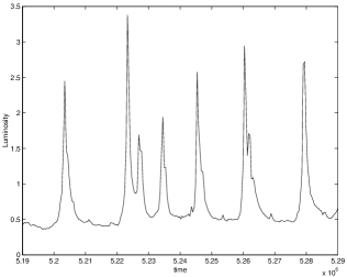
What can be noticed, in particular, from this figure is the shape of the time variation curve. A single oscillation starts with the disc luminosity $L$ that increases very steeply; then, after having reached a maximum, $L$ decreases more slowly (with an exponential-like behavior) until a value close to the initial one is reached.
We also evaluated the gas velocity field, finding a significant difference between the radial speeds ( $V_{r}$) in the two states: in the unstable region the refilled disc has a higher radial speed (with a large spread) than the collapsed one. This is what we can expect considering that the refilled disc is more luminous (since it is hotter) and therefore the accretion rate of its inner region is larger with respect to the collapsed disc. A larger accretion rate can be the effect of a larger radial speed. In fig. 6 the radial profiles of $V_{r}$ in the two states are shown.

Figure 6: The gas radial speed is shown versus $r$ in the two states (the high and the low one) of the disc. On the $x$ axis the $r$ values in units of $R_{g}$ are represented. On the $y$ axis the radial speed values in units of $c$ are represented.

It is evident from this figure what we have said above and also that in the refilled state the radial speed is often positive, besides very high. If a large radial speed is present in both inflow and outflow directions, as clearly shown in the figure, we can argue that there is a gas circulation and not only a large net accretion rate.
We highlight that this result excludes the possibility that, in 2D, a Shakura-Sunyaev disc can show a regular radial flow. This simplified one-dimensional picture is destroyed by the presence of convective and circulatory motions in the $r-z$ plane. These motions can be considered as a new turbulence, different from the one that gives rise to the $\alpha$-viscosity: the equations of the disc dynamics contain a viscosity term (the $\alpha$-term) that is physically considered the result of a supposed turbulent motion, but a disc simulated according to these equations develops another turbulent motion (that can be supposed to give rise to an additional viscosity). Our results about circulation and convection and our hypothesis that these 2D motions can be at the origin of an additional viscosity agree with the analytical study by Kippenhahn and Thomas on convective and circulatory flows in thin radiative accretion discs (Kippenhahn & Thomas, 1982). The large radial speed has also to be considered the reason for which the thermal instability causes the disc collapse and not its expansion. The local perturbative approach in itself allows to conclude that a small temperature deviation from the equilibrium state, an increase as well as a decrease, grows exponentially in time. Therefore the result should be, with the same probability, an expansion or a collapse. What we observe, instead, is that collapse is strongly preferred: in each cycle, initially the inner zone reduces largely its vertical thickness, then it swells reaching a thickness value not much larger than the equilibrium one. Our hypothesis is that what lacks in the local perturbative approach is the radial drift of matter, and therefore energy, due to the advective motion. This radial flow, carrying away thermal energy from a disc region at a certain $r$ before the expansion instability has developed at that radius, inhibits the local thermal energy growing and therefore the disc expansion.

For the case ’b’ we show the $r$-$z$ profiles of the disc particles in the two states in figs. 7 and 8. In particular, in fig. 8 we also show the boundaries of the corresponding Shakura-Sunyaev disc, from which the reader will be able to see the good agreement, in the vertical thickness, between our simulation and the canonical disc model.

Figure 7: The $r$-$z$ profile of the disc of case ’b’ in its low state is shown at the time $t=0.1016946\ 10^{7}\ R_{g}/c$ . Every SPH particle is represented by a small cross. On the $x$ axis the $r$ values in units of $R_{g}$ are represented. On the $y$ axis the $z$ values in units of $R_{g}$ are represented.

Figure 8: The $r$-$z$ profile of the same disc case ’b’ in its high state at the time $t=0.1167006\ 10^{7}\ R_{g}/c$ is shown. The solid line represents the equivalent Shakura-Sunyaev model.

The reader will notice that the whole disc is geometrically thinner in a state than in the other one. The unstable region is no more a small zone close to the black hole, as in case ’a’, but extends throughout the entire simulation radial range. This is due to the higher (supercritical) accretion rate, that makes the radiation pressure dominated zone much wider than in case ’a’. The extension of the unstable region is also apparent from the comparison between the radial profiles of the ratio $P_{rad}/P_{gas}$ in the two states, shown in fig. 9, and from the similar comparison for the temperature profiles, shown in fig. 10, where the temperature radial profile (in the disc midplane) of the corresponding Shakura-Sunyaev model is also included (in order to show also here the good degree of agreement between simulations and 1D models).

Figure 9: The ratio $P_{rad}/P_{gas}$ at the times $t=0.1016946\ 10^{7}$ and $t=0.1167006\ 10^{7}$ is shown. On the $x$ axis the $r$ values in units of $R_{g}$ are represented. The configuration at the earlier time exhibits a smaller ratio $P_{rad}/P_{gas}$ than the configuration at the later time.

Figure 10: The temperature radial profile at the times $t=0.1016946\ 10^{7}$ and $t=0.1167006\ 10^{7}$ is shown. On the $x$ axis the $r$ values in units of $R_{g}$ are represented. On the $y$ axis the temperature values in kelvin are represented. The configuration at the earlier time exhibits a smaller temperature than the configuration at the later time. The solid line represents the temperature radial profile for the equivalent Shakura-Sunyaev model.

In fact, in both figures the two profiles associated to the two states are significantly different in the whole disc: approximately up to $200R_{g}$, where the disc mass is injected, the geometrically thinner configuration is cooler and less radiation pressure dominated than the other one (the disc remains however radiation pressure dominated). So what we said about the ’a’ case is also valid in the ’b’ one: we can conclude that there is a limit-cycle oscillation between two different disc states, one thinner, cooler and therefore less luminous and the other one thicker, hotter and therefore more luminous. The luminosity oscillation is shown in fig. 11. In this figure the luminosity time behavior is represented during the entire formation and evolution of the disc from the time $t=0$, when particles begin to be injected in a totally empty space.

Figure 11: The time behavior of the disc luminosity is shown. On the $x$ axis the time values in units of $R_{g}/c$ are represented. On the $y$ axis the luminosity values in units of $L_{theor}=0.06\dot{M}c^{2}=2.05\cdot 10^{39}\hskip 5.69046pterg\hskip 5.69046ptsec^{-1}$ are represented.

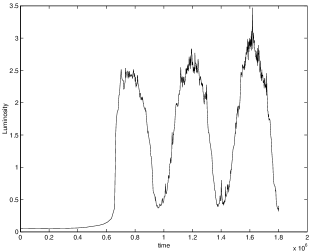
It is evident from this figure the rather different shape of the time variation curve with respect to the analogous curve for the ’a’ case. Here the luminosity $L$ increases approximately as steeply as it then decreases. So there is no exponential-like behavior as there is in the ’a’ case. We guess that this difference in the luminosity behavior is due to the much larger extension of the unstable zone in the ’b’ case. In fact, the cooling of a given disc portion is probably governed by a law closer to the exponential one if the energy density of the considered disc region is fundamentally uniform throughout the region itself. If we indicate with $E(r,t)$ the local energy density at the radius $r$ and the time $t$ in the disc, the cooling law at the position $r$ is $\frac{dE(r,t)}{dt}=-kE(r,t)$, that has for solution the exponential form for $E(r,t)$.
It is obvious that this argument holds for the total energy of an entire disc region only if the variable $E(r,t)$ to consider in the equation above is the same for the whole disc region, i.e. the energy density $E(r,t)$ is uniform in the considered region.

It is easy to notice that the oscillation shape in the ’b’ case is more similar to the light curves obtained in 1D simulations (see, for example, Watarai & Mineshige (2003), Nayakshin et al. (1985) and Szuszkiewicz & Miller (2001)) than the luminosity behavior of the ’a’ case. Our hypothesis to explain this fact is that in the ’b’ case the unstable zone is much wider. So the mass to be unloaded by the disc to pass to the collapsed state is larger. Because of this the refilled state duration is greater and the oscillation shape shows a luminosity maximum characterized by a width approximately equal to the minimum duration. In fact, we have, in the ’b’ case, two states with luminosities different by a factor 7 whose durations are about 25 $s$ each one.
In the ’a’ case, instead, when the luminosity maximum is reached the light curve starts immediately its descending (exponential) phase: the disc holds for a very short time the refilled state, probably because the disc gets soon rid of the small amount of matter contained in the small unstable zone.

Finally, we studied the radial behavior of the Mach number $M=\frac{V_{r}}{v_{s}}$.

We present the results of this analysis in the figs. 12 and 13, regarding respectively the collapsed and the refilled state. For clarity the figures show only the innermost disc region. It is clear from these figures that the disc has a sonic point, positioned nearly at $r=10R_{g}$ in the collapsed state and (very approximately) at $r=15R_{g}$ in the refilled one. From the external boundary to the sonic point the radial flow is subsonic, whereas from the sonic point to the internal boundary we have a supersonic flow. Though here our data are strongly scattered, we can say that our 2D simulated models reveal a transonic region at radii larger than in 1D calculations. For a comparison with 1D models on this aspect of the disc dynamics, one can see, for example, Szuszkiewicz & Miller (1998), where the sonic point is given around $r=3R_{g}$.

Figure 12: The radial profile of the Mach number $M=\frac{V_{r}}{v_{s}}$ for the disc of case ’b’ in its collapsed state. Every SPH particle is represented by a small cross. On the $x$ axis the $r$ values in units of $R_{g}$ are represented. On the $y$ axis the Mach number values are represented.

Figure 13: The radial profile of the Mach number $M=\frac{V_{r}}{v_{s}}$ for the disc of case ’b’ in its refilled state. Every SPH particle is represented by a small cross. On the $x$ axis the $r$ values in units of $R_{g}$ are represented. On the $y$ axis the Mach number values are represented.

5 Discussion

In this section we discuss three items:

1) confirmation by a true 2D approach of the limit-cycle behavior produced by the thermal instability;

2) differences between the results obtained by the two approaches 1D and 2D;

3) theoretical considerations about the main features of the luminosity time behavior: oscillations amplitude, typical times.

1) As we said in the first section, the limit-cycle behavior due to the Shakura-Sunyaev instability has already been shown as result of 1D time-dependent simulations (Szuszkiewicz & Miller, 1997, 1998, 2001; Janiuk et al., 2002). In this work we confirm the existence of the limit-cycle behavior using a 2D approach, obviously closer to the physical reality of accretion discs. Moreover, the 2D approach allows to reveal aspects of the accretion flow that cannot be simulated by the 1D methodology. Convection and circulation are the main ones. Also, convective motions are supposed to reduce the thermal instability (Shakura et al., 1978). Just in presence of a significant convective flow, that our 2D simulations reveal, we confirm the existence of the thermal instability.

2) In figs. 14 and 15 we show the gas velocity field in a given disc region for the two disc states. The considered case is the ’b’ one.

Figure 14: The gas velocity field in the radial range between $33R_{g}$ and $53R_{g}$ is shown for case ’b’. The disc state is the high one. On the $x$ axis the $r$ values in units of $R_{g}$ are represented. On the $y$ axis the $z$ values in the same units are represented. The arrows represent the velocity vectors, with their lengths proportional to the speed values.

Figure 15: The gas velocity field in the radial range between $33R_{g}$ and $53R_{g}$ is shown for case ’b’. The disc state is the low one. On the $x$ axis the $r$ values in units of $R_{g}$ are represented. On the $y$ axis the $z$ values in the same units are represented. The arrows represent the velocity vectors, with their lengths proportional to the speed values.

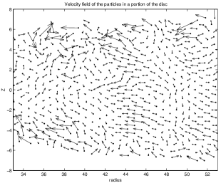
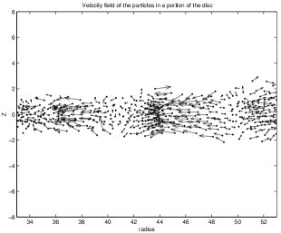
These figures make clear the different feature of the two states (high and low) as regards the convective motions in the disc. From fig. 14 we can argue the relevant presence of convective and circulatory motions in the high state, whereas from fig. 15 it is evident the poor convection in the low state.

These phenomena are important because they affect the time values that characterize the luminosity behavior. We note that the light curve we obtain is different from the curves usually obtained by 1D simulations. The luminosity behavior we find is approximately periodic, as in 1D simulations, but, in case ’a’, we obtain recurrent bursts of time duration not much smaller than the cycle-time (of about $2$ s), whereas in 1D simulations the bursts duration is very short in comparison with the cycle-time.

Moreover, convection and circulation also affect the unstable zone extension: this zone is not the full A zone, extending up to $30R_{g}$, but only a portion of it (up to $13R_{g}$), since the convective motion stabilizes a large fraction of the radiation pressure dominated region.

In case ’b’, the low and high states have about the same duration (one half of the cycle-time, that is, on average, $50$ s). In 1D simulations, instead, the high state has an extremely short duration.

Also, we have compared the disc structures we obtained from our simulations with the corresponding configurations calculated from the one-dimensional Shakura-Sunyaev model. The agreement between the results of the two approaches (the 2D simulated model and the 1D theoretical one) is in general good (see figs. 2 and 4 for case ’a’ and 8 and 10 for case ’b’), taken into account that we have a time varying disc structure. The only significant differences regard the innermost disc regions: for case ’a’, between 10 and 20 $R_{g}$, the thickness calculated from the canonical model is about 2 times the one of the simulated disc, and also the theoretical 1D temperature is larger than the simulated one (by 30 $\%$ about); for case ’b’, from 3 to 15 $R_{g}$, the thickness calculated from the canonical model is about 2-3 times the one of the simulated disc, while the theoretical 1D temperature is larger than the simulated one by 30-35 $\%$ about. So we confirm the result of Hurè and Galliano (Hurè & Galliano, 2001), who compared vertically averaged (i.e. 1D) models of accretion discs with the corresponding vertically explicit (i.e. 2D) configurations and found that the one-dimensional description of the accretion discs structure is very close to the two-dimensional one. The generally good agreement between the disc structures we simulated and the Shakura-Sunyaev model allows us to conclude that the different features between the thermal instability we found in 2D and the limit-cycle behavior obtained by the 1D calculations are not due to differences in the used disc configurations.

3) There are two time-scales that affect the time features of the limit-cycle phenomenon: the thermal time-scale, that determines the development rate of the thermal instability, and the viscous time, that is connected to the A zone refilling after the collapse due to the instability. Here we discuss the role of these time-scales for the case ’a’. In this disc the collapsing zone extends nearly from $3R_{g}$ to $13R_{g}$. We give the values of the thermal and viscous time-scales at three points in this zone. These time-scales are quantities calculated from the theoretical formulae using the values of the disc physical variables resulting from the simulation. The expression we use for the viscous time-scale is $t_{visc}=r^{2}/\nu$ and, for the thermal time-scale (Shakura & Sunyaev, 1976):

$$t_{therm}=\frac{1}{\alpha\Omega}\frac{A(\beta_{r})}{6(5\beta_{r}-3)}$$ (27)

where $A(\beta_{r})=8+51\beta_{r}-3\beta_{r}^{2}$ and $\beta_{r}=P_{rad}/P^{tot}$.

Since the viscous time depends on the disc thickness, it assumes different values in the low (collapsed) state and the high (refilled) one. So we will distinguish its values in the two states using the labels ’LS’ (Low State) and ’HS’ (High State).

$r$	$t_{visc}(LS)$	$t_{visc}(HS)$	$t_{therm}$
$3R_{g}$	$108.9$ s	$7.00$ s	$4.84\cdot 10^{-3}$ s
$7R_{g}$	$2717$ s	$6.79$ s	$2.218\cdot 10^{-2}$ s
$13R_{g}$	$25545$ s	$63.86$ s	$6.046\cdot 10^{-2}$ s

It is easy to see that the theoretical viscous time-scales are too large compared to the ’experimental’ luminosity cycle-time, whereas the thermal time-scales are too small.

We propose the following explanations. When the disc is in the low state, the accretion rate in the collapsed zone is small, but, at the outer boundary of this region, the disc is not collapsed and has a higher accretion rate. Because of this fact, the accretion flow at the outer boundary of the collapsed zone ’forces’ matter to enter the region at a rate larger than the rate due to the viscous time-scale computed inside the region itself. So the refilling process is accelerated and its time-scale reduced with respect to the viscous time. A rough estimate of this effect can be given by the value of the viscous time-scale of the disk just outside the collapsed zone. Moreover, the calculation of this viscous time-scale has to take account of the ’real’ viscosity present in the disc: the gas 2D motions (convection and circulation) give rise to a turbulent flow and consequently to an additional viscosity, of the order of magnitude $Hv_{turb}$ (where $v_{turb}$ is the speed of the turbulent flow), that has to be added to the Shakura-Sunyaev one.
To understand this procedure it must be remembered that, supposing a viscosity due to a turbulence (the Shakura-Sunyaev $\alpha$-viscosity), we have not obtained a regular flow with the turbulence ’hidden’ in the $\alpha$-viscosity term. The flow produces another turbulence, not included in the $\alpha$-viscosity term. Therefore, to express the total kinematic viscosity, we have to sum the term given by the speed of this new turbulence to the standard $\alpha$-term. In formulae, we have a total kinematic viscosity given by:

$$\nu=\alpha v_{s}H+Hv_{turb}$$ (28)

With this expression for the viscosity, the viscous time-scale $t_{visc}$ is given by:

$$t_{visc}=\frac{r^{2}}{\nu}=\frac{r^{2}}{\alpha v_{s}H+Hv_{turb}}$$ (29)

An approximate estimate for $v_{turb}$ can be obtained by adding the gas radial and vertical speeds. These formulae give for $t_{visc}$ the value of $12$ s. Finally, it has to be considered that the transition from the low to the high state is also accelerated by the process of the radial diffusion of radiation, whose typical time-scale is $\Delta t=\frac{3\tau\Delta l}{c}$, where $\Delta l$ and $\tau$ are the length and the optical depth of the region through which the radiation diffuses. Taking account of all these effects, the characteristic time of the transition LS-HS is lowered from $12$ s to about $5$, value not far from the luminosity cycle-time we obtain in case ’a’ ($2$ s).
As regards the inverse process, i.e. the transition from the high to the low state due to the thermal instability, we form the hypothesis that the instability development time, that is essentially the thermal time-scale, is increased by convection (Shakura et al., 1978). Convection is naturally simulated by our 2D code, whereas the 1D codes, obviously, cannot track the convective motions of the fluid masses and therefore do not include convection. This could be the reason for which, in 1D simulations, the high state duration is very short: the thermal time-scale is not increased by convection and therefore the instability develops very rapidly, causing the collapse of the high state in the low one in a very short time.
To support this hypothesis refer to fig. 6 for the radial speed in the two states low and high. It is clearly shown the extremely low radial speed of the collapsed zone together with the close ’active’ zone exhibiting larger radial speeds. An oscillatory radial behavior of $V_{r}$ is also evident.
It is interesting that Szuszkiewicz and Miller also found similar radial speed profiles (Szuszkiewicz & Miller, 2001), with significant oscillations in the behavior versus $r$. They claim that these oscillations are a numerical effect and, as a proof of that, show that, if an artificial diffusion is introduced, the oscillations disappear. We think, instead, that the radial speed oscillations are a real physical phenomenon, connected to the gas circulation in the disc, and that an artificial diffusion can obviously smooth away the oscillatory behavior, but this is only an artificial result due to a not physical ingredient.
Finally we want to highlight the differences between our results and Szuszkiewicz and Miller’s ones (Szuszkiewicz & Miller, 2001) about the hot gas bulge generated by the thermal instability. In their work this bulge is just the medium by which the instability propagates through the disc. When the instability arises, a small region near the black hole becomes thicker and hotter. Its thickness and temperature become larger and larger while the radial extension also increases. The hot gas bulge that is formed through this process reaches a radial extension of $90R_{g}$, then it begins to go down in the region near the black hole. The cooling wave that accompanies this process propagates gradually towards the internal boundary, until the whole gas bulge has returned to the disc equilibrium values of thickness and temperature. In our simulations the situation is different. The instability starts with the inner region collapse (therefore with the gas cooling) and not with the thickness and temperature increasing (the inverse processes). Both the collapse and the subsequent refilling are approximately simultaneous over all the unstable region: no heating and cooling waves propagate through the disc. When the unstable region is refilled, something similar to the hot bulge of Szuszkiewicz & Miller (2001) is formed. The involved region swells, but much less than in Szuszkiewicz & Miller’s simulation. It reaches a vertical thickness not much larger than the equilibrium value and, as said, does not expand radially.

6 Conclusions

We put forward evidence with true 2D simulations that the limit-cycle behavior produced by the Shakura-Sunyaev instability is present in accretion discs having a radiation pressure dominated zone (A zone). The time-scale of the instability and the shape of the light curve depend on the accretion rate. Lower accretion rates produce shorter time-scales of the oscillations.

The 2D real motions play an important role to calculate the appropriate values of the oscillation frequencies. We obtain, for the subcritical regime (case ’a’), a frequency $\nu$ of about 0.5 $Hz$ and, in the supercritical case (the ’b’), $\nu\approx 0.02$ $Hz$. In general the 2D time-scales are shorter (and the frequencies higher) than the 1D ones. We attribute this result to the shorter viscous time-scale characteristic of the zone outside the collapsed region and to the role of the large convection present in the high state.

These results may be relevant for the explanation of QPO emission in black hole candidates. More refined models are necessary for a detailed interpretation of QPO observational data, which, however, is not the purpose of this paper. Our aim is not to find an explanation of some sources behavior, but simply to see what happens to the standard disc structure during its time evolution.

References

- Bisnovatyi-Kogan & Blinnikov (1977) Bisnovatyi-Kogan G.S., Blinnikov S.I., 1977, A&A, 59, 111
- Brookshaw (1994) Brookshaw L., 1994, Mem.S.A.It., 65, n. 4, 1033
- Chakrabarti & Molteni (1993) Chakrabarti S.K., Molteni D., 1993, ApJ, 417, 671
- Dilts (1996) Dilts G.A., 1996, Los Alamos National Laboratory Report LA-UR, 96-134
- Hubeny (1990) Hubeny I., 1990, ApJ, 351, 632
- Hurè & Galliano (2001) Hurè J.-M., Galliano F., 2001, A&A, 366, 359H
- Janiuk et al. (2002) Janiuk A., Czerny B., Siemiginowska A., 2002, ApJ, 576, 908J
- Kippenhahn & Thomas (1982) Kippenhahn R., Thomas H.-C., 1982, A&A, 114, 77
- Mihalas & Klein (1982) Mihalas D., Klein R.I., 1982, Jou. Comp. Phys., 46, 97
- Molteni et al. (1998) Molteni D., Gerardi G., Valenza M.A., Lanzafame G., Ed. by Chakrabarti S.K., 1998, Observational Evidence for Black Holes in the Universe, Kluwer A.P., Dordrecht
- Monaghan (1985) Monaghan J.J., 1985, Comp. Phys. Repts., 3, 71
- Monaghan (1992) Monaghan J.J., 1992, Annu. Rev. Astron. Astrophys., 30, 543
- Nayakshin et al. (1985) Nayakshin S., Rappaport S., Melia F., 2000, ApJ, 535, 798N
- Nelson & Papaloizou (1994) Nelson R.P., Papaloizou J.C.B., 1994, MNRAS, 270, 1N
- Paczynski & Wiita (1980) Paczynski B., Wiita P.J., 1980, A&A, 88, 23
- Shakura & Sunyaev (1976) Shakura N.I., Sunyaev R.A., 1976, MNRAS, 175, 613
- Shakura et al. (1978) Shakura N.I., Sunyaev R.A., Zilitinkevich S.S., 1978, A&A, 62, 179
- Shapiro et al. (1976) Shapiro S.L., Lightman A.L., Eardley D.M., 1976, ApJ, 204, 187
- Szuszkiewicz & Miller (1997) Szuszkiewicz E., Miller J.C., 1997, MNRAS, 287, 165
- Szuszkiewicz & Miller (1998) Szuszkiewicz E., Miller J.C., 1998, MNRAS, 298, 888
- Szuszkiewicz & Miller (2001) Szuszkiewicz E., Miller J.C., 2001, MNRAS, 328, 36
- Teresi et al. (2003) Teresi V., Molteni D., Toscano E., 2003, preprint (astro-ph/0307480)
- Watarai & Mineshige (2003) Watarai K., Mineshige S., 2003, preprint (astro-ph/0306548)