Faint Galaxies in Deep ACS observations

Abstract

We present the analysis of the faint galaxy population in the Advanced Camera for Surveys (ACS) Early Release Observation fields VV 29 (UGC 10214) and NGC 4676. These observations cover a total area of 26.3 arcmin², and have depths close to that of the Hubble Deep Fields in the deepest part of the VV 29 image, with $10\sigma$ detection limits for point sources of $27.8$, $27.6$ and $27.2$ AB magnitudes in the $g_{F475W}$, $V_{F606W}$ and $I_{F814W}$ bands respectively.

Measuring the faint galaxy number count distribution is a difficult task, with different groups arriving at widely varying results even on the same dataset. Here we attempt to thoroughly consider all aspects relevant for faint galaxy counting and photometry, developing methods which are based on public software and that are easily reproducible by other astronomers. Using simulations we determine the best $SExtractor$ parameters for the detection of faint galaxies in deep HST observations, paying special attention to the issue of deblending, which significantly affects the normalization and shape of the number count distribution. We confirm, as claimed by Bernstein, Freedman and Madore (2002a,b; hereafter BFM), that Kron-like magnitudes, such as the ones generated by $SExtractor$, can miss more than half of the light of faint galaxies, what dramatically affects the slope of the number counts. We show how to correct for this effect, which depends sensitively not only on the characteristics of the observations, but also on the choice of $SExtractor$ parameters.

We present catalogs for the VV 29 and NGC 4676 fields with photometry in the $F475W,F606W$ and $F814$ bands. We also show that combining the Bayesian software BPZ with superb ACS data and new spectral templates enables us to estimate reliable photometric redshifts for a significant fraction of galaxies with as few as three filters.

After correcting for selection effects, we measure slopes of $0.32\pm 0.01$ for $22<g_{F475W}<28$, $0.34\pm 0.01$ for $22<V_{F606W}<27.5$ and $0.33\pm 0.01$ for $22<m_{F814W}<27$. The counts do not flatten (except perhaps in the $F475W$ filter), up to the depth of our observations. Our results agree well with those of BFM, who used different datasets and techniques, and show that it is possible to perform consistent measurements of galaxy number counts if the selection effects are properly considered. We find that the faint counts $m_{AB}>25.5$ can be well approximated in all our filters by a passive luminosity evolution model based on the COMBO-17 luminosity function ($\alpha=-1.5$) , with a strong merging rate following the prescription of Glazebrook et al. (1994), $\phi^{*}\propto(1+Qz)$, with $Q=4$.

1. Introduction

On March 7th 2002, the Advanced Camera for Surveys (ACS, Ford et al. 1998, 2002) was installed in HST during the space shuttle mission ST-109. ACS is an instrument designed and built with the study of the faint galaxy population as one of its main goals. Here we describe the processing and analysis of some of the first science observations taken with the ACS Wide Field Camera, called Early Release Observations (EROs).

An important result obtained with the WFPC2 observations of the Hubble Deep Fields (Williams et al. 1996, Casertano et al. 2000) was the measurement of the galaxy number count distribution to very faint $(m_{AB}\gtrsim 27)$ limits. However, it is remarkable that different groups have reached different conclusions about the slope and normalization of the number counts even when using the same software on the same dataset (see e.g. Ferguson, Dickinson & Williams 2000, Vanzella et al. 2001). One of the few results on which all groups seemed to agree was the flattening of the number counts at $I_{AB}\sim 26$. However, BFM claim that this is a spurious effect, caused by the underestimation of the true luminosity of faint galaxies by standard aperture measurements, and that the number counts continue with a slope of $0.33$ up to the limits of the HDFN V and I bands.

Two of the main goals of this paper are improving our understanding of the biases and selection effects involved in counting and measuring the properties of very faint galaxies, and developing techniques that can be applied to a wide range of observations and that are easily reproduced by other astronomers. This is essential if galaxy counting is to become a precise science. We have done this by using almost exclusively public software, and specifying the parameters used, thus ensuring that our results are repeatable.

Our final results are the number counts in the $F475W$, $F606W$ and $F814W$ bands, carefully corrected for selection effects. Using an independent procedure, we confirm the apparent absence of flattening in the number counts found by BFM. We also show that using proper priors, reasonably robust photometric redshifts can be obtained using only three ACS filters. Finally, we present photometric catalogs of field galaxies in the VV 29 and NGC 4676 fields.

The structure of the paper is the following: Section 2 describes our observations, Section 3 deals with the image processing and the generation of the catalogs, including the description of the simulations used to correct our number counts. Section 4 lists and explains the quantities included in our catalogs, Section 5 presents our number counts, and Section 6 summarizes our main results and conclusions.

2. Observations

The observations analyzed here were obtained with the Wide Field Camera of the Advanced Camera for Surveys (Ford et al. 1998, 2002) and include two fields. The first is centered on VV 29 (Vorontsov-Velyaminov 1959), also known as UGC 10214 and Arp 188 (Arp 1966), a bright spiral with a spectacular tidal tail at $z=0.032$. Due to a pointing error, the field was imaged twice, resulting in a central region with twice the exposure time of the NGC 4676 field. The galaxy itself and its associated star formation has been considered in detail by Tran et al.(2002). The second field is centered on NGC 4676 (Holmberg, 1937), an interacting galaxy pair at $z=0.022$. Figures 1 and 2 show the ACS images of these fields, and Table 1 summarizes the main characteristics of the observations.

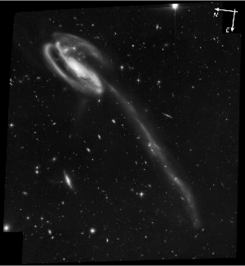
Figure 1.— Color image of VV 29, the “Tadpole”, obtained by combining the ACS WFC F475W, F606W and F814W filters. The observations are described in Table 1.

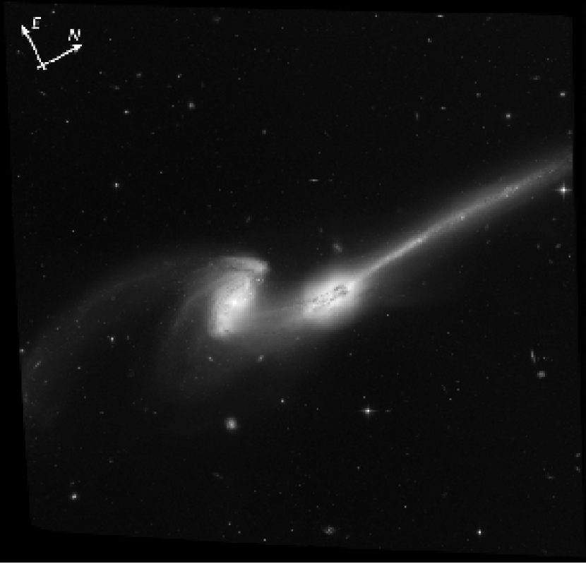
Figure 2.— Color image of NGC 4676, the “Mice” obtained by combining the ACS WFC F475W, F606W and F814W filters. The observations are described in Table 1.

Table 1Early Release Observations of VV 29(UGC 10214) and NGC 4676

Field	RA(J2000)	DEC(J2000)	ACS WFC filter	Exposure time	N exposures	Area (arcmin2)
VV 29	16:06:17.4	55:26:46	F475W	$13600$	$12$	14.48
VV 29	16:06:17.4	55:26:46	F606W	$8040$	$12$	14.49
VV 29	16:06:17.4	55:26:46	F814W	$8180$	$12$	14.46
NGC 4676	12:46:09.0	30:44:25	F475W	$6740$	$6$	11.84
NGC 4676	12:46:09.0	30:44:25	F606W	$4000$	$6$	11.84
NGC 4676	12:46:09.0	30:44:25	F814W	$4070$	$6$	11.84

3. Data analysis

3.1. Image processing

A brief description of the calibration and reduction procedures for the VV 29 field can be found in Tran et al. (2003). The raw ACS data were processed through the standard CALACS pipeline (Hack 1999) at STScI. This included overscan, bias, and dark subtraction, as well as flat-fielding. CALACS also converts the image counts to electrons and populates the header photometric keywords. About half of the images in these datasets were taken as cosmic ray (CR) split pairs that were combined into single “crj” images by CALACS; the rest were taken as single exposures.

The calibrated images were then processed through the “Apsis” ACS Investigation Definition Team pipeline, described in detail by Blakeslee et al. (2003). Briefly, Apsis finds all bright compact objects in the input images, sorts through the catalogs to remove the cosmic rays and obvious defects, corrects the object positions using the ACS distortion model (Meurer et al. 2003), and then derives the offsets and rotations for each image with respect to a selected reference image. For the present data sets, over one hundred objects were typically used in deriving the transformation for each image, and the resulting alignment errors were about 0.04 pix in each direction. The relative rotation between the first and second epoch VV 29 observations was found to be 0$\fdg$12. The offsets and rotations were then used in combining the individual frames to produce single geometrically corrected images for each bandpass.

Image combination in Apsis is done with the drizzle software written by R. Hook (Fruchter & Hook 2002). The data quality arrays enable masking of known hot pixels and bad columns, while cosmic rays and other anomalies are rejected through the iterative drizzle/blot technique described by Gonzaga et al. (1998). For these observations, we used the “square” (linear) drizzle kernel with an output scale of 0$\farcs$05 pix^-1. The full width at half maximum (FWHM) of the point spread function (PSF) was about 0$\farcs$105, or 2.1 WFC pixels. The linear drizzling of course correlates the noise in adjacent pixels, decreasing the root-mean-squared (RMS) noise fluctuations per pixel by a factor $1-\frac{1}{3l}$ for our parameters, where $l$ is the linear size of the area in which the fluctuations are measured (Casertano et al. 2000). However, Apsis calculates RMS arrays for each drizzled image, i.e., the expected RMS noise per pixel in the absence of correlation. These arrays are used later on for image detection, photometric noise estimation, etc.

Figure 3 shows the behavior of the noise as a function of the size of the area in which it is measured. We see that it follows well the predicted behavior, but it is slightly higher on large scales, an effect which was also noted in the HDFS by Casertano et al. 2000, and is probably due to intrinsically correlated fluctuations in the background galaxy density.

Figure 3.— Behavior of the empirically measured noise in apertures of varying size (solid line) vs. the expected one (dashed line), for the central part of the VV 29 F475W images, based on the drizzle parameters and the noise model of Casertano et al. 2000. As in the case of the HDFN, the measured noise is higher than the prediction. Similar behavior is observed in the other filters.

In addition Apsis detects and performs photometry of stars and galaxies in the images using $SExtractor$ (Bertin & Arnouts 1996) and obtains photometric redshifts for galaxies using the software BPZ (Benítez 2000), steps which will be described in detail below.

The stellar FWHM of our images, $\sim 0\farcs 105$ is significantly better than that of WFPC2 observations (e.g., $\sim 0\farcs 14$ for the HDFS). A detailed analysis of the ACS WFC point spread function (PSF) will be published elsewhere (Sirianni et al., in preparation). Table 2 shows the $10\sigma$ limiting magnitudes for the deep central area of VV 29 (which was imaged twice), and for the outer area of the VV 29, together with the NGC 4676 field.

The absolute accuracy of the positions derived from the information in the ACS image header is limited to $\sim 1\arcsec$ by the uncertainty in the guide star positions and the alignment of the ACS WFC to Hubble’s Fine Guidance Sensors. As a last step, we correct the astrometry of the images using the software wcstools and the Guide Star Catalog II (Mink et al. 2002). Although there are not many cataloged stars in our images, visual inspection shows that our corrected positions should be accurate to $\lesssim 0\farcs 1$.

Table 2Depth of the VV 29 and NGC 4676 fields compared with the HDFS

	VV 29	VV 29/NGC 4676	HDFS
F475W	27.61 (27.83)	27.23 (27.45)	27.97 (27.90)
F606W	27.42 (27.64)	27.09 (27.31)	28.47 (28.40)
F814W	26.98 (27.20)	26.58 (26.80)	27.84 (27.77)

Note. — Limiting magnitudes for our fields and the HDFS. In each entry, the numbers on the left represent the expected $10\sigma$ fluctuation in an 0.2 arcsec² square aperture. The number in parenthesis corresponds to the same quantity, but within a circular aperture that has a diameter 4 times the FWHM of the PSF. We use a value of $0\farcs 105$ arcsec for the WFC observations and $0\farcs 135$ for the HDFS (Casertano et al. 2000). The circular apertures allow a realistic comparison of the limiting magnitudes for point sources. The ACS stellar limiting magnitude through the $4\times$ FWHM aperture ($d\sim 0\farcs 42$) is $\sim 0.22$ magnitudes fainter than a source filling the $0\farcs 45\times 0\farcs 45$ rectangular aperture, whereas the equivalent WFC2 stellar limiting magnitude is $\sim 0.07$ magnitudes brighter because of the WFC2’s broader PSF.

The reduced images in the three filters, together with auxiliary images (detection image, rms images) can be downloaded from http://acs.pha.jhu.edu.

3.2. Galaxy identification and photometry

3.2.1 Object detection

$SExtractor$ (Bertin & Arnouts 1996) has become the de facto standard for automated faint galaxy detection and photometry. It finds objects using a connected pixel approach, including weight and flag maps if desired, and provides the user with efficient and accurate measurements of the most widely used object properties. As stated previously, one of our main goals is to understand in detail how the process of galaxy detection and analysis affect the shape of the number counts distribution, and then use this understanding to arrive at results that are as objective as possible. To achieve our goal, we carefully choose our $SExtractor$ parameters, and most importantly, characterize the biases and errors by using extensive simulations with the public software $BUCS$ (Bouwens Universe Construction Set, see Appendix A, and Bouwens, Broadhurst, and Illingworth 2003 for a detailed description). This approach will allow other astronomers to contrast and compare our results with their own in a consistent way. Because the output of $SExtractor$ sensitively depends on its input parameters, we present our parameters in Appendix B to ensure that others can repeat our analysis.

One of $SExtractor$’s more convenient features is the double image mode. This mode enables object detection and aperture definition in one image, and aperture photometry in a different image. To create our detection image, we use an inverse variance weighted average of the $F475W$, $F606W$ and $F814W$ images. This differs from the procedure followed for the HDFs by other authors, who usually only use the reddest bands, $F606W$ and $F814W$. However, we think that inclusion of the $F475W$ image is justified since it is the deepest of the three; in fact, Table 2 shows that the $F475W$ image is almost as deep as the HDFS for point sources. The PSF in the final detection image is basically identical to that of the $F606W$ image, and differs by less than $2\%$ from the stellar width of the $B$ and $I$ filters.

Although there are roughly thirteen parameters which influence the detection process in $SExtractor$, the most critical ones are $DETECT\_MINAREA$, the minimum number of connected pixels and $DETECT\_THRESH$, the detection threshold above the background. We performed tests to select these parameters, ensuring that we recovered all obvious galaxies in the field while not producing large numbers of spurious detections. We chose the rather conservative limits of $DETECT\_MINAREA=5$ and $DETECT\_THRESH=1.5$ (which provides a nominal $S/N=3.35$), because we think that given the limited scientific information to be extracted from the sources close to the detection limit, it is better to avoid adulterating our catalogs with large numbers of false sources. Figure 4 shows the results of a $SExtractor$ run in a portion of the VV 29 field. To estimate the number of isolated spurious detections, we subtracted the mean sky and changed the sign of all pixels in our images and ran $SExtractor$ on them with the same parameters and configuration as described in Appendix B. The number of spurious detections for $m_{AB}<28$ is very small in all filters, as we can see in Figure 5, but have nevertheless been corrected for in the final number counts results.

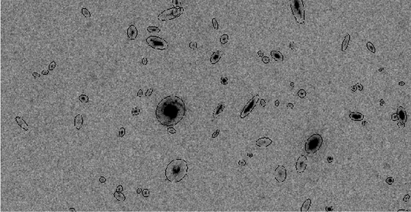
Figure 4.— Example of $SExtractor$ object finding and deblending on a section of the VV 29 field. The displayed apertures are the ones corresponding to $SExtractor$ $MAG\_AUTO$ magnitudes.

Figure 5.— Number of expected spurious detections, caused by noise caused by noise fluctuations, as a function of magnitude (see text). The thin solid line corresponds to the central part of the VV 29 field (see Table 1.), the dashed line to the outer VV 29 field and the NGC 4676 field and the thick solid line to whole field.

3.2.2 Object deblending

Two other very important parameters which govern the deblending process are DEBLEND_NTHRESH and DEBLEND_MINCONT. Typical values used by other authors are respectively $32$ and $0.01-0.03$. At least two teams using HDFN data performed part of the detection/deblending process with manual intervention (Casertano et al. 2000, Vanzella et al. 2001). This approach may be valid for an isolated field, but we think that it should not be applied to a large set of observations such as the ones which will be produced by the ACS GTO program. Not only does manual intervention require considerable effort, it also introduces subjective biases and possible inconsistencies that make repeatability by other groups difficult, as well as complicating quantification of the errors with simulations. Consequently, we decided to look for values of the deblending parameters able to perform the best possible ’blind’ detection while simultaneously keeping an eye on the biases introduced by this approach.

It soon became clear that if we wanted to avoid excessive splitting of spiral galaxies we would lose some of the faint objects close to the very brightest galaxies and stars. Because VV 29 is an exceptional field with a bright galaxy and associated tidal tail spanning the field, we decided to sacrifice the brightest galaxies by using the automatic procedure described below. The procedure generates masks which enclose the areas around bright objects in which $SExtractor$ does not work properly (see Figures 6 and 7). Thus, we were able to focus on the correct deblending of galaxies in the field.

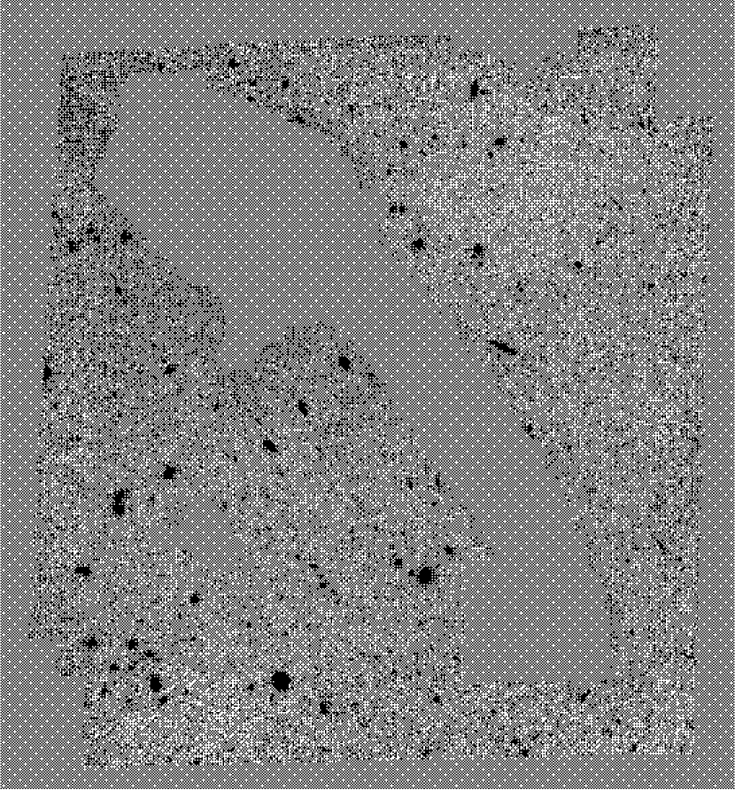
Figure 6.— Detection image for the VV 29 field obtained by combining the F475W, F606W and F814W filters weighting by the inverse of the variance, after masking the areas near bright objects where $SExtractor$ does not perform adequately (see text in Sec. 3.2.2).

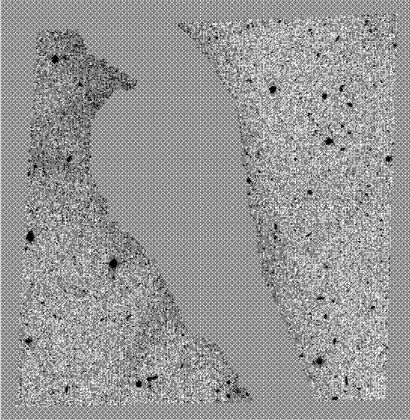
Figure 7.— Same as Fig. 6 but for the NGC 4676 field.

We first generated a simulated field with the same filters, depth, and other characteristics as our ACS observations. This was done using $BUCS$, with galaxy templates extracted from the VV 29 field itself, guaranteeing the same kind of fragmentation problems encountered in the real images. This simulated field is processed in exactly the same way as the real images, and the output $SExtractor$ catalog is matched and compared with the input catalog. A surprising result was that about $\sim 7\%$ of the input objects with $I<27$ were not present in the output catalog, in the sense that no object was detected within 0.2 arcsec of their positions. This number changed little for reasonable values of the deblending parameters. At the same time, the proportion of spurious objects (present in the output catalog but not in the input one, and formed from fragments of brighter galaxies) depended strongly on the deblending parameters, varying from $5\%$ to $17\%$. Since no choice of parameters was able to totally eliminate both effects at the same time, we decided to try to make them cancel each other out.

We ran an optimization process on the DEBLEND_NTHRESH and DEBLEND_MINCONT parameters by minimizing the difference between the magnitude distribution of spurious and “undetected” objects, $D^{2}_{su}=\Sigma[n_{s}(m)-n_{u}(m)]^{2}$. This was achieved for values of 16 and 0.025 respectively.

By definition, having $D_{su}\approx 0$ conserves the shape and normalization of the number counts. Visual inspection of the $SExtractor$ aperture maps shows that most of the parameters in this set produced very good results (see Figure 4). It should be noted that a significant part of the differences in the HDF number counts among different groups (see e.g. Vanzella 2002) may be caused by the deblending procedure. Changing DEBLEND_MINCONT from 0.025 to 0.01 and DEBLEND_NTHRESH from 16 to 32 more than doubles the numbers of spurious objects, increasing the faint number counts by $\approx 10\%$ (Figure 8). The values chosen by Casertano et al. 2002, 32 and 0.03 produce results on the ACS images quite close to the ones obtained with our optimal parameter set.

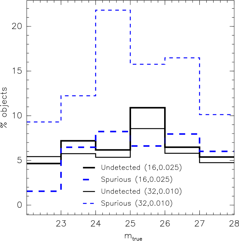
Figure 8.— Dependence of the number of spurious and undetected objects due to deblending errors as a function of magnitude for the optimal values of the $SExtractor$ parameters $DEBLEND\_MINCONT=0.025$ and $DEBLEND\_NTHRESH=16$ (see text). We also show how using different values, e.g. $DEBLEND\_MINCONT=0.01$ and $DEBLEND\_NTHRESH=32$ leaves almost unaffected the number of undetected galaxies, but more than doubles the number of spurious objects, significantly changing the normalization and shape of the number count distribution.

The parameter set chosen by us ensures that the number and magnitude distribution of galaxies in the input and output catalogs are the same. Since the objects used in the simulation are drawn from a real sample of galaxies, we hope that this will also hold for the observations. Now we turn to a delicate question, how to measure the light emitted by these galaxies.

3.2.3 Measuring magnitudes

$SExtractor$ provides a plethora of magnitude measurements. Among them are MAG_ISO, the isophotal magnitude which measures the integrated light above a certain threshold, MAG_AUTO, an aperture magnitude measured within an elliptical aperture adapted to the shape of the object and with a width of k times the isophotal radius and MAG_APER, a set of circular aperture magnitudes. The most commonly used magnitude for faint galaxy studies is MAG_AUTO, with purported accuracies of a few percent for objects detected at high signal to noise. However, BFM recently claimed that this measurement technique can be off by more than a magnitude near the detection limit.

Observational biases in faint galaxy detection and photometry hinder comparison of distant galaxy samples with lower redshift ones such as the SDSS (Yasuda et al. 2001, Blanton et al. 2003) and the 2dF (Magdwick et al. 2002). To estimate these biases we again resort to simulations performed with BUCS. Using the final VV 29 and NGC 4676 images, we “sprinkle” galaxies with the same redshift, colors, and magnitude distribution as the objects present in the HDFN onto both fields. We use HDFN templates instead of VV 29 since the former have much better color and redshift information, and therefore allow us to recreate with better accuracy realistic galaxy fields; to avoid overcrowding we use a surface density of only $20\%$ of the observed surface density. Finally we analyze the simulated images in the same way as the real images. Because we are interested in comparing the recovered or “observed” magnitudes with the “true” ones, we create galaxies with analytical profiles that have a distribution as similar as possible to the HDFN real galaxies. We repeat this procedure until $\sim 10000$ galaxies have been added to the NGC 4676 and VV 29 fields. As expected, we confirm that MAG_AUTO estimates total magnitudes much better than MAG_ISO or MAG_APER for reasonable values of the apertures, but there is still a significant amount of light being left out. We fit 5-order polynomials to the median filtered $m_{auto}-m_{true}$ vs $m_{auto}$ data. The results are shown in Figure 9. We see that our corrections do not rise as dramatically with magnitude as those of BFM, perhaps because we are using quite conservative parameters for MAG_AUTO, an aperture of $2.5$ times the isophotal radius, and a minimal radial aperture of 0.16 arcsec for faint objects. Nevertheless, there is an actual overall dependence on the depth, especially at very faint magnitudes, where the corrections for the ’shallow’ VV 29 field and the NGC 4676 field are systematically larger than that of the ’deep’ VV 29. The dependence of the correction on magnitude is quite similar for all filters, and we do observe a ’pedestal’ effect which affects even objects with $m\sim 20$. In all filters, the correction increases rapidly when approaching the detection limit of the field, so one has to be very careful in drawing conclusions about derived quantities like the luminosity function when using data close to the detection magnitude limit.

Figure 9.— Aperture corrections, defined as the difference between the total ’intrinsic’ magnitudes and the $SExtractor$ $MAG\_AUTO$ magnitude. The thick line corresponds to the central part of the VV 29 field (see Table 1.), and the thin line to the combination of the outer VV 29 field and the NGC 4676 field. Note that the behavior is similar in the relatively high S/N regime, but quickly differs at faint magnitudes.

3.2.4 Color estimation

Accurately measuring the colors of a galaxy is often a different problem than measuring its total magnitude. In our case, where all filters have very similar PSFs, using a single aperture defined by the detection image guarantees that magnitude measurements in all filters will be affected by the same systematic errors which cancel out when subtracting the magnitudes to calculate the colors. We again tested several of the $SExtractor$ measurements and concluded that colors based on MAG_ISO provide the best estimate of a galaxy’s “true” colors (provided, of course, that the object colors inside the isophotal threshold are similar to those outside of it). There seem to be two reasons for this; first, using an isophotal aperture is more efficient, in terms of signal–to–noise, than $MAG\_AUTO$, which integrates the light distribution over regions where the noise is dominant. Second, although $SExtractor$ tries to correct its aperture magnitude measurements for the presence of nearby objects, it does not always do so successfully, and there are a significant number of cases where the magnitudes are strongly contaminated by the light from close companions. Isophotal magnitudes are largely free of this problem. The comparisons between MAG_ISO and MAG_AUTO are shown in Figure 10. For bright, compact objects a small aperture with a diameter of 0.15 arcsec works slightly better than MAG_ISO, but its performance is equal or slightly worse for fainter objects, so we decided to use MAG_ISO for all objects.

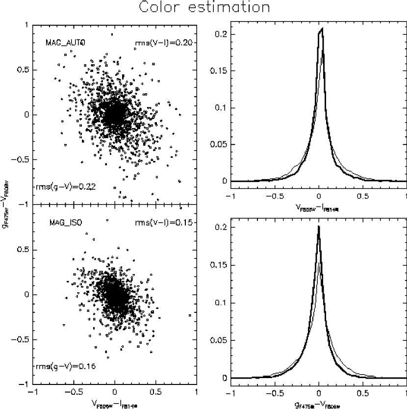
Figure 10.— On the left plots, the X-axis shows the difference between the $V-I$ color measured by SExtractor, and the intrinsic or ’true’ colors of the galaxies. The Y-axis shows the same quantity, but for the $g-V$ color. The bottom left plot corresponds to isophotal and the top left plot to Kron magnitudes. Only $20\%$ of the points are plotted for clarity. Note that the scatter is considerably smaller for isophotal magnitudes. The right plots display the color distributions as histograms. The top right plot for the $V-I$ colors and the bottom right plot for the $g-V$ ones. The thick line corresponds to the isophotal colors, the thin line to the Kron ones.

As expected, the advantages of isophotal magnitudes for estimating colors also are evident in the photometric redshifts. On average, we can estimate reliable photometric redshifts for $11\%$ more objects if we use MAG_ISO instead of MAG_AUTO (see Sec. 3.3).

We show color-color plots, together with the tracks corresponding to some of the templates introduced below, in Figure 11.

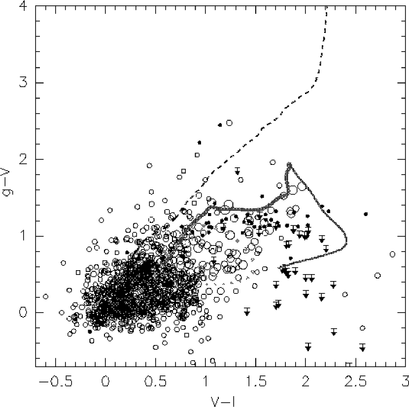
Figure 11.— Color-color plot in the VV 29 and NGC 4676 fields. Filled circles represent objects with star class $\geq 0.94$ (i.e. likely to be stars), arrows correspond to objects not detected in the $F475W$ filter (we show their $2\sigma$ detection limits), and open circles represent galaxies, with the size proportional to their magnitude (the largest ones are $I\approx 18$). The solid line corresponds to the $z<2$ color track of an elliptical galaxy, the dotted line to an Sbc with $z<3$ and the dashed line to a starburst. The thicknesses of the curves decrease with redshift. For clarity, we only plot $50\%$ of the galaxies.

3.2.5 Completeness corrections

We previously noted that $SExtractor$ is not designed to work near very bright objects and in general will produce numerous spurious detections while missing obvious real objects. We are experimenting with a wavelet-based method to fit the background that may alleviate the need to perform such steps in the future (White et al., in preparation). However, at present we must work around this problem in order to avoid significantly biasing our estimation of the number count distribution. We masked out areas around bright objects by using an automatic procedure. First we ran $SExtractor$ and identified only those objects with areas larger than 20,000 pixels, which are the ones that typically cause problems with deblending. The mask was created by setting all pixels outside these object to one, and all interior pixels to zero. To create a “buffer zone” around these objects, we convolved the mask with a 15 pixel boxcar filter. In the case of VV 29 we additionally masked a small area by hand which contained obvious contamination from star clusters belonging to VV 29 itself. The final areas that remained after applying the masking are shown in Figures 6 and 7. The objects in the masked areas are included in the catalog, but are flagged to show that they are in a masked area where $SExtractor$ is likely to produce incomplete results.

One additional problem is that $SExtractor$’s probability of detecting an object depends not only on its magnitude, but also on its size, surface brightness, and other parameters. To measure the incompleteness as a function of magnitude, we again used the simulations described in Sec. 3.2.2. We confirmed that the masking procedure has adequately excluded all the areas where the galaxy detection is compromised by bright objects. The resulting detection efficiency is shown in Figure 12.

Figure 12.— Fraction of galaxies detected for each of the filters versus total magnitude. The thick line corresponds to the central region of the VV 29 field, and the thin line corresponds to the outer region of the VV 29 field plus the NGC 4676 field. Note that the X-axis corresponds to the ’total’ intrinsic magnitudes

3.3. Photometric redshifts

The deep, multi-color HDFN observations provided a strong impetus for developing and using photometric techniques to estimate the redshifts of faint galaxies. The relatively large number of galaxies that now have ground-based redshifts provide a benchmark for testing different photometric redshift methods. The most widely used HDFN photometric catalog is that of Fernández-Soto et al. 1999, which includes PSF matched photometry of the WFPC2 $UBVI$ and ground based $JHK$ bands.

Photometric redshift techniques can be broadly divided into those which use a library of spectral energy distributions (SED), and the “empirical” methods, which try to model the color-redshift manifold in a non-parametric way (see Benítez 2000, Csabai et al. 2003 for a detailed discussion). The latter require abundant spectroscopic redshifts, and are therefore more appropriate for low redshift samples such as the Sloan Digital Sky Survey (Csabai et al. 2003).

For faint galaxy samples like the ones presented here, and in general for ACS observations, the only options are SED-based techniques, for which a critical issue is the choice of the template library. At first sight it may seem most logical to use synthetic galaxy evolution models, like the Bruzual & Charlot (1993) ones (used in Hyper-z, Bolzonella, Miralles & Pelló 2000) or the Fioc & Rocca-Volmerange (1997) ones, since they take into account age effects, dust extinction, etc. However, simple tests quickly showed that the most effective SEDs for photometric redshift estimation are obtained from observations of real galaxies, e.g. a subset of the Coleman, Wu and Weedman (1980) (CWW) spectra augmented with two Kinney et al. (1996) starbursts ( Benítez 2000, Csabai et al. 2003, Mobasher et al. in preparation). But even these templates have shortcomings. A detailed comparison of the colors predicted by the CWW+SB templates and those of real galaxies in several spectroscopic catalogs show small but significant differences. We developed a method to trace these differences back to the original templates, and model them using Chebyshev polynomials, generating a new set of “calibrated” templates which produce much better results in independent samples. We show these new templates, together with the original extended CWW set in Figure 13. A detailed description of this technique will be given elsewhere.

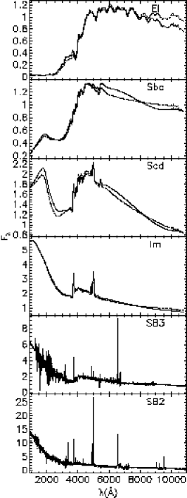
Figure 13.— The thick lines show “calibrated” templates (see text), used for photometric redshifts. The thin lines correspond to the CWW and Kinney et al. 1996 original templates.

Many observers assume that measuring accurate photometric redshifts requires as many as five or more filters. However, as we show here, useful redshift information can be derived from as few as three filters by using a Bayesian approach. The problem of determining photometric redshifts can be stated as (Benítez 2000):

$$p(z|C,m_{0})=\sum_{T}p(z,T|C,m_{0})\propto\sum_{T}p(z,T|m_{0})p(C|z,T)$$ (1)

where $z,C$ and $m_{0}$ are respectively the redshift, colors and magnitude of a galaxy, and $T$ corresponds to the templates, or spectral energy distributions (SED) used to estimate its colors. The term $p(C|z,T)$ is the likelihood, and the differences between Bayesian photometric redshifts and maximum-likelihood or $\chi^{2}$ ones arise from the presence of the prior $p(z,T|m_{0})$ and the marginalization over all the template types. The redshift-type prior is neither more nor less than the expected redshift distribution for galaxies of a given spectral type as a function of magnitude. It contains what we know about a galaxy’s redshift and type just by looking at its magnitude. In most cases this is very little, of course, but it is obvious that using this information is just translating common sense to a mathematical form: brighter galaxies tend to be at lower redshifts than fainter ones.

There is a persistent prejudice that using a prior will “bias” the redshift estimate, making the data unfit for various scientific applications like measurement of the luminosity function, whereas maximum likelihood estimates are free of such problems. It is easy to show that this is completely unjustified from the point of view of probability theory. It is clear that using maximum likelihood is similar, in this particular setting, to using a “flat” prior, i.e., $p(z,T|m_{0})=const$. This means that using maximum likelihood (or equivalently $\chi^{2}$) is not assumption-free; on the contrary, it is similar to assuming that the redshift distribution of galaxies is flat at all magnitudes. To obtain such an observed redshift distribution one has to contrive a luminosity function with enormous evolution rates, therefore tending to significantly “overproduce” the number of high-z galaxies. This is clearly shown in our tests below (see Figure 14).

Figure 14.— Comparison between spectroscopic and photometric redshifts obtained using, using basically the same filter set as the VV 29 and NGC 4676 observations. Note that the axes are inverted with respect to the typical orientation in this kind of plot. This is done to better show the effects of using photometric redshifts to select galaxy samples. In the case of Maximum Likelihood photometric redshifts, almost one third of the $z>1.5$ objects would be misclassified low redshift objects, biasing high any estimate of the the luminosity function, star formation rate, etc. obtained with them. The dashed line has slope 1 and it does not represent a fit to the data. The filled circles correspond to the objects classified as outliers in Table 3. Note that since the axis are inverted, the outliers were selected based on their horizontal distance to the dashed line with respect to the rms fluctuation.

Table 3Performance of Bayesian and Maximum Likelihood photometric redshift methods

sample	$n_{gal}$	mean	rms	$n_{out}$
$z<1.5$, bayesian	73	-0.002	0.073	5
$z<1.5$, max.likelihood	58	-0.018	0.133	3
$z>1.5$, bayesian	16	0.004	0.081	3
$z>1.5$, max.likelihood	31	-0.04	0.126	11

Ideally one would want to use the ’real’ redshift distribution $p(z,T|m_{0})$ of the field as the prior, but this is usually unknown, since it is the quantity we want to measure. But it is clear that an analytical fit to the redshift histogram from a similar blank field, like the HDFN, is always a much better approximation—in spite of the cosmic variance—than a flat redshift distribution. Thus using empirical priors such as the ones introduced in Benítez (2000), does in fact considerably reduce the biases introduced by maximum-likelihood methods. Simple comparisons like the one below using the same dataset and template sets show that, as expected, Bayesian probability gives consistently more accurate and reliable results than maximum-likelihood or $chi^{2}$ techniques (see also Benítez 2000, Csabai et al. 2003, Mobasher et al. in preparation).

To test how well we can expect to estimate photometric redshifts with our data, we performed the following test. We ran BPZ with the same set of parameters described in Appendix C, but using only the WFPC2 BVI photometry from the Fernández-Soto et al. 1999 catalog. This is almost identical in filter coverage and depth to the observations discussed here, and therefore serves as an excellent test of the performance of our photometric redshifts. The results, both for the Bayesian ($z_{B}$) and maximum likelihood photometric redshifts ($z_{ML}$) are shown in Figure 14 and Table 3. In the lower plot we excluded those objects with Bayesian odds $O<0.9$ (Benítez 2000), about $1/3$ of the sample, and performed a similar preselection for $z_{ML}$ by excluding the objects with the highest values of $\chi^{2}$, up to $1/3$ of the total. We see that despite this pruning of the data, the number of “catastrophic” maximum likelihood outliers (error $\geq 3\sigma$) seriously affects any scientific analysis, especially in the $z>1.5$ range, where $1/3$ of the objects selected using Maximum Likelihood photometric redshifts happen to be low-redshift galaxies. This is a good example of the tendency to overproduce the number of high$-z$ galaxies of the maximum likelihood or $chi^{2}$ methods discussed above.

We also performed a test based on the simulations described above to determine the “efficiency” of our photometric redshifts as a function of magnitude and redshift. We looked at the number of galaxies with Bayesian odds $O>0.9$ in the output of the simulations described in the section above as a function of total magnitude in the $F814W$ band, $I_{total}$, and ’true’ redshift. The results are shown in Figures 15 and 16. They show that, using this limited filter set, we can only expect to estimate reliable photometric redshifts for bright, $I\lesssim 24$ objects, and only for certain regions of the redshift range. This should be taken into account when using the photometric redshifts in the catalog. Figure 17 compares the redshift distribution in our fields with that of the HDFN for galaxies with $I_{F814W}<24$.

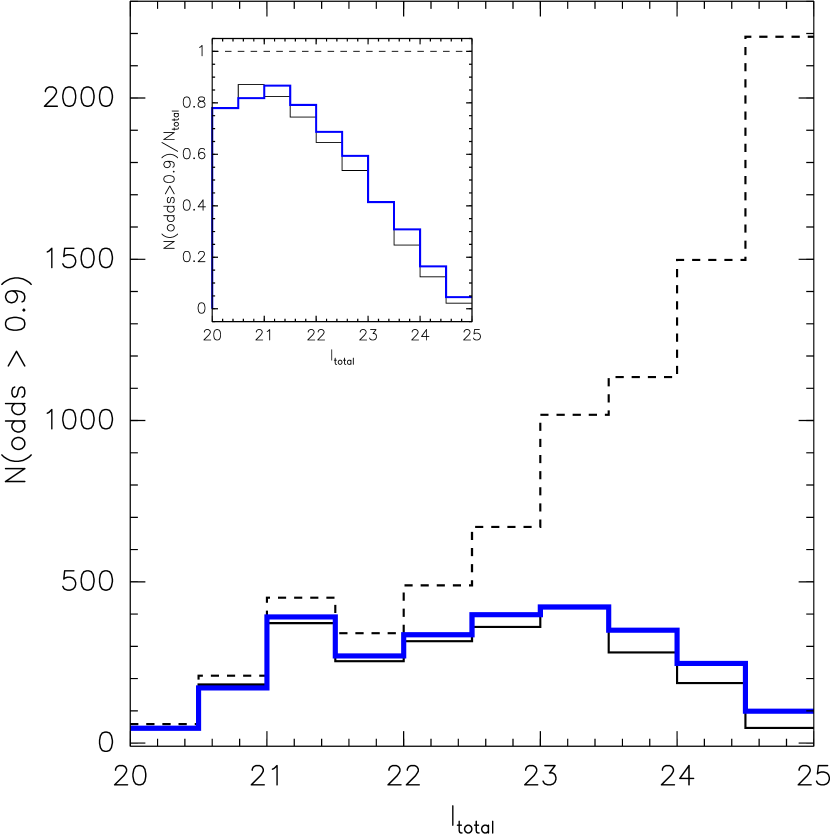
Figure 15.— Distribution of galaxies with Bayesian $odds>0.9$ (photometric redshifts with lower values are unreliable) in our simulations as a function of magnitude. This shows that there are few objects with good quality photometric redshifts for $I\gtrsim 24.5$. The thick line corresponds to isophotal magnitudes, and the thin line to Kron apertures; the figure shows that isophotal magnitudes improve the accuracy of the photometric redshifts. The dashed line corresponds to the total number of objects.

Tables 6 and 7 give the photometric and positional information for those objects whose photometric redshifts have very high values of the Bayesian odds, and which therefore can be expected to be quite accurate and reliable. Based on previous experience and comparison with other catalogs such as the HDFN, we expect an rms accuracy of $\approx 0.1(1+z)$ and only a few percent of objects with “catastrophic” redshift errors. We also provide photometric redshift information for the rest of the objects in both fields as explained below, but we note here that, as BPZ indicates, their redshifts are much more uncertain.

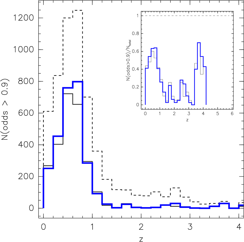
Figure 16.— Redshift distribution of $I<25$ galaxies. The meaning of the different types of lines are the same as in the previous figure.

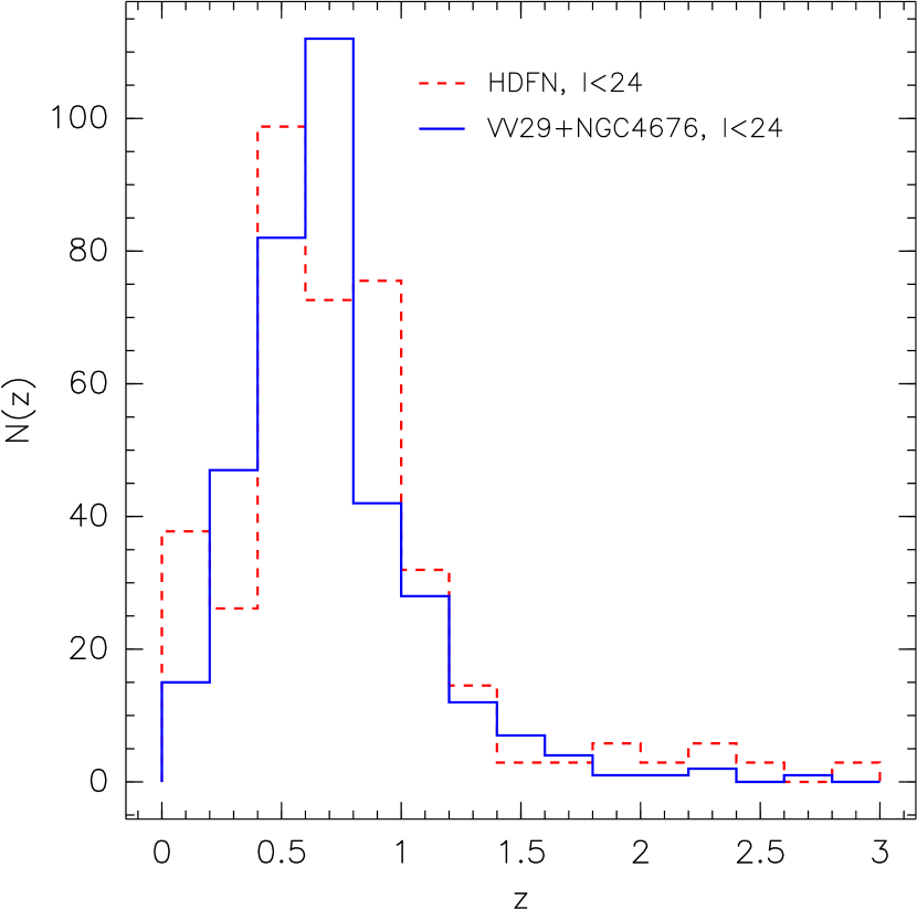
Figure 17.— Comparison between the redshift distribution of all the galaxies with $I<24$ in our observations (solid line) and the HDFN (dashed line) scaled to our total effective area.

3.4. The catalogs

For each of the fields observed by ACS we provide two catalogs which will be published electronically and also made available at the ACS website (http://acs.pha.jhu.edu).

3.4.1 Photometric Catalog

These catalogs contain all the objects detected by $SExtractor$ in each of the fields. We decided not to purge the spurious detections, but effectively eliminated them by selecting only objects with $mask\_flag=0$. The photometric catalog contains the following columns:

- $ID$. This is the $SExtractor$ ID number in the output catalog.

- $RA,DEC$. These are the right ascension and declination, calibrated with the Guide Star Catalog II. They have relative accuracies of $\lesssim 0\farcs 1$.

- $X,Y.$ Pixel coordinates in the images.

- $g_{auto},V_{auto},I_{auto}$. These are $SExtractor$, uncorrected Kron elliptical magnitudes $MAG\_AUTO$. They should be used as the best estimate of the total magnitude of a galaxy, although they miss an increasingly large fraction of the light at faint magnitudes. But, as argued above, for color estimation or photometric redshifts we recommend isophotal magnitudes.

- $g_{iso},V_{iso},I_{iso}$. These are $SExtractor$ isophotal ($MAG\_ISO$) magnitudes.

- $FWHM$. Full width at half maximum in pixels, recalling that the scale of the images is $0\farcs 05$ pixel^-1.

- $starclass$. $SExtractor$ star/galaxy classifier. We consider as stars or point sources all objects which have a value of this parameter $\geq 0.94$, and set all their photometric redshift parameters to zero.

- $flag$. $SExtractor$ detection flag.

- $maskflag$. If the value of this flag is 1, it indicates that the object is in an area strongly affected by incompleteness or the presence of spurious objects. For most science uses only objects with $maskflag=0$ should be selected.

3.4.2 Photometric redshift Catalog

We estimated Bayesian photometric redshifts for galaxies in our catalog using the parameters specified in Appendix C. The main difference relative to the method presented in Benítez 2000 is that we used the template library described above. For a more detailed discussion, see Benítez 2000.

- $z_{b}$. Bayesian photometric redshift, or maximum of the redshift probability distribution.

- $z_{b}^{min},z_{b}^{max}$. Lower and upper limits of the redshift probability $95\%$ confidence interval. Note that in some cases, this probability distribution is multimodal, so these values or $z_{b}$ are not very meaningful.

- $t_{b}$. Bayesian spectral type. The types are El (1), Sbc(2), Scd(3), Im(4), SB3(5), and SB2(6).

- $odds$. Bayesian odds. This is the integral of the redshift probability distribution in a region of $\approx 0.2(1+z_{b})$. If close to 1, it means that the redshift probability is narrow and has a single peak. Very low values of the odds indicate that the color/magnitude information is almost useless to estimate the redshift.

- $z_{ml}$. Maximum likelihood redshift. We provide this to allow users to compare with the value of $z_{b}$, and also to understand the effects of the prior on the redshift estimate. As an estimate of the redshift we recommend the use of $z_{b}$, which has been proved to be more accurate and reliable.

- $t_{ml}$. Maximum likelihood spectral type.

- $\chi^{2}$. This is the value corresponding to the maximum likelihood redshift/spectral type fit.

4. Number counts

Our number counts are shown in Figure 18 and listed in Table 4. We plot the raw number counts, as measured by $SExtractor$, the aperture corrected counts as described in Section 3.2.3, and finally correct for spurious detections and incompleteness to estimate the final number counts. The result can be very well fitted by a straight line with slopes $0.32\pm 0.01$, $0.34\pm 0.01$ and $0.33\pm 0.01$ respectively in the $F475W$, $F606W$ and $F814W$ bands (Table 5). This is in excellent agreement with the results of BFM, who measure slopes of $0.33\pm 0.01$ and $0.34\pm 0.01$ respectively in the $F606W$ and $F814W$ bands. The normalization is in remarkably good agreement too, taking into account the size of the fields and the very different correction procedures followed.

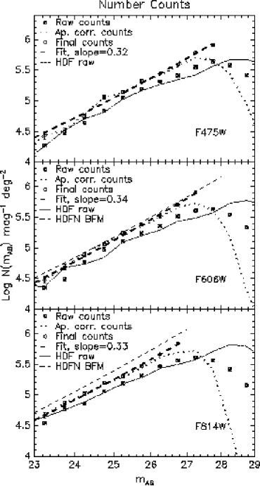
Figure 18.— Number counts distributions. The filled squares , the dotted line is our counts after applying aperture corrections, and the open circles show the final number counts after correcting for incompleteness. The thick dashed line is a least square fit to the open circles. The continuous thin lines are the number counts in the HDFS+HDFN (Casertano et al. 2000). In the two bottom plots we also show the corrected counts from Bernstein, Freedman & Madore 2002, which have slopes and normalizations close to our results even though they were obtained with a different approach.

There is a significant difference in the raw number counts between our data and the HDF’s, of about $40\%$ in the g and V bands and $20\%$ in the I band, in the sense that we find more objects than Casertano et al. (2000). Although $1/4$ of this difference goes away when we use a detection image formed by only our V and I images (instead of $gVI$), most of the difference is probably due to the fact that our PSF is more compact, with significantly less light at large radii than for WFPC2. Therefore the apertures used by $MAG\_AUTO$ will enclose more of the light from each galaxy, creating a steepening effect similar to the one produced by the aperture corrections. To test for possible contamination from star clusters belonging to the central galaxies, we mapped the distribution of extended objects with colors similar to obvious star clusters. Since they are distributed homogeneously across the field and are not particularly concentrated toward the central galaxies, they are probably not a large contaminant.

Table 4Number Counts

	$g_{F475W}$				$V_{F606W}$				$I_{F814W}$
$m_{AB}$	$N$	$N_{raw}$	$dN_{raw}$		$N$	$N_{raw}$	$dN_{raw}$		$N$	$N_{raw}$	$dN_{raw}$
23.25	27177	18909	3103		30072	22486	3384		46166	34751	4209
23.75	31849	30152	3920		48467	30663	3953		73853	59282	5499
24.25	55978	43950	4734		77776	58771	5475		103432	71547	6041
24.75	115058	68481	5910		115580	95056	6964		158452	113454	7609
25.25	140421	112943	7592		177131	129297	8123		202678	154339	8876
25.75	213130	154339	8876		239108	172737	9390		292149	208511	10317
26.25	277901	205955	10254		321145	227420	10775		459216	295901	12292
26.75	390832	259105	11502		508518	326054	12903		689457	368472	13717
27.25	616540	353651	13438		799663	405268	14386		1282821	406290	14404

Note. — Corrected numbers counts $N(m)$ in the three filters. We also present the raw number counts $N_{raw}(m)$, based on the $MAG\_AUTO$ magnitudes provided by SExtractor, and their $\sqrt{(}N)$ errors for comparison. The raw counts are measured on a $14.1$ arcmin² area, but all quantities are normalized to 1 sq. degree area

Table 5Number count slopes

Filter	$\alpha$	mag. range	$\alpha_{BFM}$	mag. range (BFM)
$F475W$	$0.32\pm 0.01$	$22<m_{AB}<28$	-	-
$F606W$	$0.34\pm 0.01$	$22<m_{AB}<27.5$	$0.33\pm 0.01$	$22<m_{AB}<27$
$F814W$	$0.33\pm 0.01$	$22<m_{AB}<27$	$0.34\pm 0.01$	$22<m_{AB}<27$

Note. — Slopes for number count fits of the form $N(m)\propto 10^{\alpha m}$, both for the results presented in these paper and those of Bernstein, Freedman and Madore (2002a,b). We also include the magnitude interval on which the fit was performed.

Galaxy number counts (especially at very faint magnitudes) provide important constraints on galaxy formation and evolution (Gronwall & Koo 1995). We compare our results with some simple galaxy number count generated using the public software ncmod (Gardner 1998) in Figure 19.We make use of the recently derived $B$-band luminosity function from the COMBO-17 survey (Wolf et al. 2003), derived at $z\sim 0.3$ and which features a rather steep slope ($\alpha=-1.5$) for the faint end of the luminosity function. We assume a flat, $\Omega_{\Lambda}=0.7$ cosmology with $H_{0}=70$ km s^-1 Mpc^-1. We generate K+e corrections using GISSEL96 synthetic templates (Bruzual & Charlot 1993). This pure luminosity evolution model works reasonably well for magnitudes brighter than $25$ in all bands, but drops significantly below the observed counts at fainter magnitudes, falling short by a factor of $\sim 2$ by $m\sim 27$. It is clear that our data have reached the magnitude levels at which merging (as expected by hierarchical models of galaxy formation) is important. Thus, we also plot the predictions of two luminosity evolution models with simple (and rather strong) merging prescriptions. Guiderdoni & Rocca-Volmerange (1990) proposed a merging rate of (1+z)^η, with $\eta=1.5$, but their predicted counts also fall short of our measurements. Following Broadhurst, Ellis & Glazebrook (1992), Glazebrook et al. (1994) proposed a model where the merging rate is proportional to $1+Q\times z$. We use $Q=4$ (such that a present day galaxy is the result of a merger between $\sim 4$ sub-units at $z\sim 1$.) and find that this prescription fits well the counts in the $m_{AB}>25.5$ range, producing a distribution which has the measured slopes and normalization in all our bands.

Figure 19.— Comparison with number count models. The points correspond to our final corrected number counts (same as the open squares in the previous plot). The thick solid line represents a no-evolution model and the dashed line a passive luminosity evolution (PLE) model. The dotted and dotted-dashed line represent PLE models including merger of galaxies following respectively the Guiderdoni & Rocca-Volmerange (1990) and the Broadhurst, Ellis & Glazebrook (1990) prescriptions. The thin solid line represents the LCDM predictions of Nagashima et al. (2002). See the text for details about the model generation and comments.

Finally, we also include the hierarchical model predictions of Nagashima et al. (2002) which, although include both the luminosity evolution and merging (as predicted by hierarchical formation theory) of galaxies, also underpredict the observed number counts by a factor of $\sim 2$.

The color distribution of galaxies with magnitude also provides important constraints on galaxy evolution models. Figure 20 shows the observed and median galaxy colors as a function of magnitude. The typical color of detected $I\approx 28$ galaxies is $g-V\sim V-I\sim 0.15$ are similar to those of blue starbursting galaxies at $1.2\leq z\leq 2.6$, as expected from the results of Benítez 2000 for the redshift distribution of faint galaxies in the HDFN.

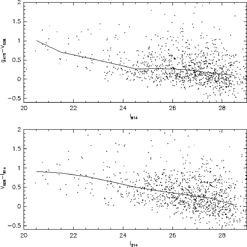
Figure 20.— Median color as a function of magnitude. The upper and lower figures show respectively the $g-V$ and $V-I$ isophotal colors of galaxies plotted as a function of their $MAG\_AUTO$ $I$ magnitude. The solid lines represent the median color of the galaxies.

We would like to note that although the prediction of the Glazebrook et al. (1994) model fits the data satisfactorily, any result of this kind is very sensitive to the choice of luminosity function parameters, and that in any case it is very unlikely that the evolution of the galaxy population is will be described by such a simple scheme. Although it is beyond the scope of this paper to explore more sophisticated models of galaxy number counts, we hope that these new data and our effort to remove instrumental biases and other corrections which hinder the measurement of the number count distribution will aid future modeling efforts.

5. Conclusions

We present the analysis of the faint galaxy population in the Advanced Camera for Surveys (ACS) Early Release Observation fields VV 29 (UGC 10214) and NGC 4676. These were the first science observations of galaxy fields with ACS and show its efficiency compared with the previous Hubble Space Telescope optical imaging preferred instrument, WFPC2. The observations cover a total area of 26.3 arcmin², with an effective area for faint galaxy studies of 14.1 arcmin², and have depths close to that of the Hubble Deep Fields in the central and deepest part of the VV 29 image, with $10\sigma$ detection limits for point sources of $27.8$, $27.6$ and $27.2$ AB magnitudes in the $g_{F475W}$, $V_{F606W}$ and $I_{F814W}$ bands respectively.

The measurement of the faint galaxy number count distribution is still a somewhat controversial subject, with different groups arriving at widely varying results even on the same dataset. Here we attempt to thoroughly consider all aspects relevant for faint galaxy counting and photometry, developing methods which are based on public software like $SExtractor$ and $BUCS$, and therefore easy to reproduce by other astronomers.

Using simulations we determine the best $SExtractor$ parameters for the detection of faint galaxies in deep HST observations, paying special attention to the issue of deblending, which significantly affects the normalization and shape of the number count distribution. We also confirm, as proposed by BFM, that Kron-like ($MAG\_AUTO$) magnitudes, like the ones generated by $SExtractor$, can miss more than half of the light of faint galaxies. This dramatic effect, which strongly changes the shape of simulated number count distributions, depends sensitively not only on the characteristics of the observations, but also on the choice of $SExtractor$ parameters, and needs to be taken into account to make meaningful comparisons with theoretical models or between the results of different authors.

We present catalogs for the VV 29 and NGC 4676 fields with photometry in the $F475W,F606W$ and $F814$ bands. We show that combining the Bayesian software BPZ with superb ACS data and new templates enables us to estimate reliable photometric redshifts for a significant fraction of galaxies with as few as three filters.

After correcting for selection effects we find that the faint number counts have slopes of $0.32\pm 0.01$ for $22<g_{F475W}<28.$, $0.34\pm 0.01$ for $22<V_{F606W}<27.5$ and $0.33\pm 0.01$ for $22<I_{F814W}<27$, and do not flatten (except perhaps in the $F475W$ filter), up to the depth of our observations. Our results agree well with those that BFM obtained with different datasets and techniques ($0.33\pm 0.01$ for $22<V_{F606W}<27$ and $0.34\pm 0.01$ for $22<I_{F814W}<27.$). This is encouraging, and shows that it is possible to perform consistent measurements of galaxy number counts if the selection effects are properly taken into account.

While some may argue that any corrections–even well motivated ones such as those we use here–are model dependent, given the magnitude of the selection effects, applying some correction is better than none at all, as the widely varying results on faint galaxy number counts demonstrate. We have presented a methodology based on freely available software that enables a consistent comparison across different datasets and against theoretical results.

We compare our counts with some simple traditional number count models using the software $ncmod$ (Gardner 1998). At brighter magnitudes ($m_{AB}<25$) the counts are well approximated by a passive luminosity evolution model based on the steep slope ($\alpha=-1.5$) quasi-local luminosity function from the COMBO-17 survey. This model underpredicts the faint end by a factor $\sim 2$, and it is necessary to introduce the merging prescription of Glazebrook et al (1994), $\phi^{*}\propto(1+Qz)$, which with $Q=4$ produces good fits to both the slope and number count normalization at $m_{AB}>25.5$ in all our filters.

Table 6Photometric Redshift catalog in the VV 29 field

ID	RA	DEC	X	Y	$z_{b}$	$g_{F475W}$	$V_{F606W}$	$I_{F814W}$	FWHM	s
33	16:06:15.69	55:28:01.7	1276.2	171.7	$0.48_{-0.20}^{+0.20}$	$22.46\pm 0.01$	$21.77\pm 0.01$	$21.32\pm 0.00$	0.49	0.04
102	16:06:25.37	55:26:53.4	3415.4	234.9	$1.22_{-0.29}^{+0.29}$	$25.01\pm 0.07$	$23.57\pm 0.02$	$21.96\pm 0.01$	0.29	0.03
127	16:06:28.55	55:26:30.0	4128.2	270.6	$0.66_{-0.22}^{+0.22}$	$22.98\pm 0.01$	$22.42\pm 0.01$	$21.77\pm 0.00$	1.13	0.03
198	16:06:23.32	55:27:01.5	3039.8	322.6	$1.35_{-0.31}^{+0.31}$	$25.32\pm 0.03$	$25.44\pm 0.03$	$25.42\pm 0.03$	0.14	0.34
201	16:06:21.53	55:27:13.1	2657.3	326.1	$1.86_{-0.38}^{+0.38}$	$25.22\pm 0.02$	$25.45\pm 0.03$	$25.66\pm 0.03$	0.15	0.15
241	16:06:18.27	55:27:22.3	2107.1	524.0	$0.38_{-0.18}^{+0.18}$	$21.61\pm 0.01$	$20.73\pm 0.00$	$20.28\pm 0.00$	0.25	0.03
275	16:06:19.79	55:27:18.6	2356.3	422.5	$0.60_{-0.21}^{+0.21}$	$25.70\pm 0.06$	$25.16\pm 0.03$	$24.61\pm 0.02$	1.37	0.00
297	16:06:15.65	55:27:44.9	1477.8	441.5	$0.72_{-0.22}^{+0.22}$	$26.80\pm 0.11$	$26.03\pm 0.06$	$25.09\pm 0.03$	0.70	0.00
343	16:06:23.45	55:26:49.0	3211.7	507.1	$0.52_{-0.20}^{+0.20}$	$23.36\pm 0.01$	$22.63\pm 0.01$	$22.11\pm 0.01$	0.14	0.04
347	16:06:14.94	55:27:46.1	1367.3	496.4	$1.38_{-0.31}^{+0.31}$	$23.57\pm 0.01$	$23.74\pm 0.01$	$23.77\pm 0.01$	0.75	0.03
389	16:06:21.45	55:26:57.2	2842.8	585.7	$0.69_{-0.22}^{+0.22}$	$23.55\pm 0.02$	$22.55\pm 0.01$	$21.48\pm 0.00$	0.40	0.03
416	16:06:12.27	55:27:58.3	860.0	584.5	$0.80_{-0.24}^{+0.24}$	$25.20\pm 0.04$	$24.71\pm 0.03$	$23.80\pm 0.01$	1.07	0.00
442	16:06:21.32	55:26:56.1	2838.4	617.9	$1.87_{-0.38}^{+0.38}$	$25.63\pm 0.03$	$26.01\pm 0.04$	$26.31\pm 0.06$	0.34	0.03
446	16:06:01.09	55:24:57.7	1579.7	4606.0	$0.67_{-0.22}^{+0.22}$	$25.68\pm 0.06$	$24.55\pm 0.02$	$23.35\pm 0.01$	0.27	0.03
467	16:06:01.41	55:24:55.9	1644.9	4602.1	$0.86_{-0.24}^{+0.24}$	$24.62\pm 0.04$	$23.50\pm 0.01$	$22.18\pm 0.01$	0.22	0.03
471	16:06:00.96	55:24:58.8	1548.5	4603.4	$2.75_{-0.49}^{+0.49}$	$24.05\pm 0.02$	$23.96\pm 0.01$	$24.28\pm 0.02$	0.76	0.03
584	16:06:02.42	55:24:49.5	1859.5	4596.8	$0.51_{-0.20}^{+0.20}$	$23.19\pm 0.01$	$22.12\pm 0.01$	$21.33\pm 0.00$	0.26	0.03
677	16:06:03.96	55:24:52.2	2032.8	4393.1	$0.76_{-0.23}^{+0.23}$	$26.21\pm 0.08$	$25.39\pm 0.04$	$24.32\pm 0.02$	0.23	0.03
689	16:06:03.68	55:24:56.0	1948.9	4363.0	$0.98_{-0.26}^{+0.26}$	$24.03\pm 0.03$	$23.15\pm 0.01$	$21.87\pm 0.01$	0.74	0.02
725	16:06:14.40	55:23:46.6	4241.3	4333.3	$0.68_{-0.22}^{+0.22}$	$26.58\pm 0.06$	$25.89\pm 0.03$	$25.12\pm 0.02$	0.24	0.03
737	16:06:03.49	55:24:57.6	1903.3	4355.7	$0.64_{-0.22}^{+0.21}$	$25.19\pm 0.04$	$24.63\pm 0.03$	$24.01\pm 0.02$	0.51	0.03
796	16:05:58.07	55:25:38.2	676.5	4282.4	$1.87_{-0.38}^{+0.38}$	$23.74\pm 0.02$	$23.99\pm 0.02$	$24.31\pm 0.03$	3.53	0.00
813	16:06:14.11	55:23:48.9	4173.7	4328.4	$0.33_{-0.17}^{+0.17}$	$22.72\pm 0.01$	$22.19\pm 0.00$	$21.96\pm 0.00$	1.76	0.03
819	16:06:04.99	55:24:42.7	2288.0	4434.4	$0.76_{-0.23}^{+0.23}$	$24.28\pm 0.03$	$23.30\pm 0.01$	$22.06\pm 0.01$	0.55	0.03
892	16:06:10.86	55:24:16.8	3394.6	4227.8	$1.11_{-0.28}^{+0.28}$	$24.85\pm 0.02$	$24.95\pm 0.02$	$24.66\pm 0.02$	0.47	0.03
960	16:06:13.49	55:24:03.5	3911.4	4163.1	$0.58_{-0.21}^{+0.21}$	$24.92\pm 0.03$	$23.81\pm 0.01$	$22.76\pm 0.01$	0.91	0.03
1135	16:06:16.61	55:23:50.7	4488.1	4035.9	$1.86_{-0.38}^{+0.38}$	$24.44\pm 0.02$	$24.67\pm 0.02$	$24.90\pm 0.02$	0.51	0.03
1266	16:05:58.73	55:25:58.5	515.4	3893.4	$1.25_{-0.30}^{+0.29}$	$25.45\pm 0.03$	$25.61\pm 0.03$	$25.43\pm 0.03$	0.16	0.03
1342	16:06:12.46	55:24:33.3	3406.5	3800.0	$2.74_{-0.49}^{+0.49}$	$25.78\pm 0.02$	$25.67\pm 0.02$	$26.04\pm 0.03$	0.17	0.07
1371	16:06:14.90	55:24:16.9	3936.3	3802.8	$1.26_{-0.30}^{+0.30}$	$24.41\pm 0.01$	$24.52\pm 0.01$	$24.39\pm 0.01$	0.59	0.03
1455	16:06:13.24	55:24:34.1	3500.8	3705.5	$0.58_{-0.21}^{+0.21}$	$25.88\pm 0.03$	$25.17\pm 0.02$	$24.57\pm 0.01$	0.17	0.04
1517	16:05:59.95	55:26:06.7	578.9	3637.0	$0.71_{-0.22}^{+0.23}$	$24.18\pm 0.03$	$23.47\pm 0.01$	$22.60\pm 0.01$	2.60	0.03
1520	16:06:00.04	55:26:06.0	599.6	3638.3	$0.62_{-0.21}^{+0.21}$	$26.04\pm 0.07$	$25.20\pm 0.03$	$24.42\pm 0.02$	0.81	0.00
1532	16:06:01.17	55:26:01.0	812.3	3598.8	$0.67_{-0.22}^{+0.22}$	$22.76\pm 0.01$	$22.14\pm 0.01$	$21.42\pm 0.00$	0.40	0.03
1538	16:06:16.15	55:24:19.8	4068.7	3625.5	$1.86_{-0.38}^{+0.38}$	$24.50\pm 0.01$	$24.70\pm 0.01$	$24.95\pm 0.02$	0.15	0.34
1558	16:06:00.33	55:26:07.5	620.4	3582.9	$0.74_{-0.23}^{+0.23}$	$24.43\pm 0.03$	$23.57\pm 0.02$	$22.50\pm 0.01$	0.79	0.03
1572	16:06:11.07	55:24:56.5	2935.9	3579.6	$0.52_{-0.20}^{+0.20}$	$25.64\pm 0.04$	$25.08\pm 0.02$	$24.66\pm 0.02$	0.28	0.02
1580	16:06:15.61	55:24:27.1	3905.4	3567.3	$0.62_{-0.21}^{+0.21}$	$24.04\pm 0.02$	$23.54\pm 0.01$	$22.98\pm 0.01$	2.05	0.00
1718	16:05:59.80	55:26:14.2	466.2	3533.5	$0.85_{-0.24}^{+0.24}$	$23.86\pm 0.03$	$22.60\pm 0.01$	$21.19\pm 0.00$	0.19	0.03
1746	16:06:15.50	55:24:37.5	3763.7	3415.4	$0.63_{-0.22}^{+0.21}$	$23.15\pm 0.01$	$22.77\pm 0.01$	$22.35\pm 0.01$	2.40	0.00
1827	16:06:11.99	55:25:04.1	2965.7	3363.4	$1.39_{-0.31}^{+0.31}$	$25.36\pm 0.02$	$25.56\pm 0.02$	$25.57\pm 0.03$	0.37	0.03
1921	16:06:03.72	55:26:05.6	1097.7	3258.4	$1.04_{-0.27}^{+0.27}$	$24.28\pm 0.02$	$23.32\pm 0.01$	$21.97\pm 0.01$	0.10	0.92
2079	16:06:12.58	55:25:12.9	2936.0	3161.4	$1.19_{-0.29}^{+0.29}$	$25.09\pm 0.02$	$25.24\pm 0.02$	$25.01\pm 0.02$	0.25	0.03
2155	16:06:02.66	55:26:17.8	806.4	3176.8	$0.88_{-0.25}^{+0.25}$	$24.24\pm 0.02$	$23.88\pm 0.01$	$22.98\pm 0.01$	0.40	0.03
2156	16:06:03.16	55:26:16.4	889.8	3146.4	$1.33_{-0.31}^{+0.31}$	$23.64\pm 0.01$	$23.77\pm 0.01$	$23.79\pm 0.01$	0.83	0.03
2499	16:06:15.18	55:25:13.6	3276.3	2878.5	$0.52_{-0.20}^{+0.20}$	$21.75\pm 0.01$	$20.96\pm 0.00$	$20.43\pm 0.00$	5.03	0.03
2685	16:06:15.22	55:25:16.7	3243.3	2826.5	$1.38_{-0.31}^{+0.31}$	$24.58\pm 0.02$	$24.71\pm 0.02$	$24.70\pm 0.02$	1.12	0.00
2694	16:06:10.76	55:25:49.4	2243.1	2776.5	$0.07_{-0.07}^{+0.14}$	$20.60\pm 0.00$	$20.54\pm 0.00$	$20.68\pm 0.00$	4.30	0.03
2696	16:06:19.89	55:24:39.7	4325.1	2920.1	$1.24_{-0.29}^{+0.29}$	$25.38\pm 0.03$	$25.51\pm 0.04$	$25.35\pm 0.03$	0.94	0.03
2730	16:06:06.50	55:26:17.5	1324.6	2779.8	$1.29_{-0.30}^{+0.30}$	$24.91\pm 0.02$	$24.98\pm 0.02$	$24.94\pm 0.02$	0.75	0.03
2736	16:06:05.25	55:26:25.2	1063.2	2789.5	$0.70_{-0.22}^{+0.22}$	$23.96\pm 0.02$	$23.15\pm 0.01$	$22.26\pm 0.00$	0.49	0.03
2785	16:06:05.67	55:26:26.0	1109.1	2732.7	$0.35_{-0.18}^{+0.18}$	$22.35\pm 0.01$	$21.78\pm 0.00$	$21.55\pm 0.00$	1.73	0.03
2845	16:06:11.81	55:25:47.1	2412.1	2702.8	$0.69_{-0.22}^{+0.22}$	$23.05\pm 0.01$	$22.74\pm 0.01$	$22.30\pm 0.00$	0.69	0.03
3002	16:06:03.76	55:26:47.4	591.2	2594.5	$1.87_{-0.38}^{+0.38}$	$25.06\pm 0.03$	$25.31\pm 0.03$	$25.76\pm 0.05$	1.06	0.03
3017	16:06:04.55	55:26:43.8	740.8	2568.6	$0.26_{-0.17}^{+0.17}$	$22.23\pm 0.00$	$21.95\pm 0.00$	$21.97\pm 0.00$	0.30	0.03
3091	16:06:08.44	55:26:20.7	1546.0	2526.0	$1.31_{-0.30}^{+0.30}$	$26.54\pm 0.10$	$25.45\pm 0.04$	$23.75\pm 0.01$	0.26	0.03
3094	16:06:10.55	55:26:09.4	1967.6	2483.0	$0.52_{-0.20}^{+0.20}$	$22.07\pm 0.01$	$21.15\pm 0.00$	$20.55\pm 0.00$	3.97	0.03
3108	16:06:07.92	55:26:26.2	1408.9	2494.6	$0.60_{-0.21}^{+0.21}$	$23.79\pm 0.02$	$23.27\pm 0.01$	$22.75\pm 0.01$	1.93	0.03
3117	16:06:03.03	55:26:58.1	359.8	2501.5	$0.90_{-0.25}^{+0.25}$	$23.70\pm 0.02$	$23.28\pm 0.01$	$22.26\pm 0.01$	0.13	0.04
3380	16:06:10.46	55:26:25.6	1757.2	2236.7	$0.29_{-0.17}^{+0.17}$	$21.78\pm 0.00$	$21.05\pm 0.00$	$20.66\pm 0.00$	2.04	0.03
3392	16:06:21.09	55:25:14.4	4059.9	2245.5	$1.26_{-0.30}^{+0.30}$	$25.24\pm 0.03$	$25.36\pm 0.03$	$25.23\pm 0.03$	2.08	0.00
3414	16:06:19.54	55:25:26.0	3709.0	2224.7	$0.57_{-0.21}^{+0.21}$	$23.41\pm 0.01$	$22.92\pm 0.01$	$22.47\pm 0.01$	0.89	0.03
3429	16:06:12.02	55:26:16.3	2081.6	2220.1	$1.30_{-0.30}^{+0.30}$	$23.89\pm 0.01$	$23.97\pm 0.01$	$23.92\pm 0.01$	2.09	0.00
3480	16:06:08.01	55:26:45.4	1184.9	2180.0	$1.88_{-0.38}^{+0.38}$	$24.39\pm 0.01$	$24.63\pm 0.01$	$25.12\pm 0.02$	0.65	0.03
3486	16:06:14.13	55:26:05.5	2496.7	2170.3	$0.77_{-0.23}^{+0.23}$	$24.91\pm 0.02$	$24.44\pm 0.01$	$23.62\pm 0.01$	0.36	0.03
3553	16:06:08.05	55:26:52.6	1100.9	2062.5	$0.26_{-0.17}^{+0.16}$	$21.67\pm 0.00$	$21.37\pm 0.00$	$21.32\pm 0.00$	5.35	0.00
3588	16:06:11.48	55:26:30.4	1835.5	2053.9	$0.12_{-0.12}^{+0.15}$	$22.84\pm 0.01$	$22.71\pm 0.01$	$22.71\pm 0.01$	0.26	0.03
3597	16:06:21.03	55:25:26.4	3904.3	2062.6	$1.36_{-0.31}^{+0.31}$	$25.73\pm 0.03$	$25.93\pm 0.03$	$25.91\pm 0.03$	0.24	0.02
3654	16:06:15.58	55:26:07.3	2669.8	1989.5	$0.62_{-0.21}^{+0.21}$	$23.22\pm 0.01$	$22.79\pm 0.01$	$22.31\pm 0.01$	2.60	0.00
3915	16:06:17.02	55:26:13.2	2790.1	1746.0	$1.15_{-0.28}^{+0.28}$	$25.51\pm 0.02$	$25.62\pm 0.02$	$25.37\pm 0.02$	0.42	0.03
3918	16:06:24.61	55:25:23.1	4424.8	1739.7	$1.24_{-0.29}^{+0.29}$	$24.54\pm 0.02$	$24.63\pm 0.02$	$24.49\pm 0.02$	0.53	0.03
3982	16:06:22.56	55:25:30.3	4060.7	1840.8	$1.88_{-0.38}^{+0.38}$	$25.13\pm 0.02$	$25.40\pm 0.02$	$25.81\pm 0.03$	0.19	0.03
3985	16:06:12.17	55:26:50.1	1685.4	1671.9	$0.66_{-0.22}^{+0.22}$	$24.39\pm 0.02$	$23.92\pm 0.01$	$23.31\pm 0.01$	1.51	0.03
4041	16:06:13.37	55:26:45.1	1907.3	1623.3	$1.24_{-0.29}^{+0.29}$	$25.73\pm 0.03$	$25.92\pm 0.04$	$25.71\pm 0.03$	0.79	0.02
4056	16:06:24.69	55:25:33.2	4310.5	1572.4	$0.60_{-0.21}^{+0.21}$	$23.94\pm 0.03$	$23.08\pm 0.01$	$22.34\pm 0.01$	2.74	0.00
4084	16:06:16.86	55:26:23.5	2642.4	1599.4	$1.35_{-0.31}^{+0.31}$	$25.76\pm 0.03$	$25.94\pm 0.03$	$25.89\pm 0.03$	0.24	0.03
4172	16:06:10.41	55:27:10.0	1204.6	1539.9	$0.52_{-0.20}^{+0.20}$	$26.16\pm 0.06$	$24.99\pm 0.02$	$24.07\pm 0.01$	0.82	0.00
4176	16:06:07.71	55:27:10.0	843.4	1824.2	$0.73_{-0.23}^{+0.23}$	$25.15\pm 0.02$	$24.75\pm 0.02$	$24.09\pm 0.01$	0.40	0.03
4213	16:06:17.45	55:26:26.2	2687.3	1495.1	$1.18_{-0.29}^{+0.29}$	$25.58\pm 0.03$	$25.72\pm 0.03$	$25.48\pm 0.03$	1.14	0.00
4227	16:06:17.06	55:26:29.8	2590.5	1478.1	$0.80_{-0.24}^{+0.24}$	$23.26\pm 0.01$	$22.93\pm 0.01$	$22.21\pm 0.01$	1.46	0.03
4329	16:06:15.08	55:26:48.7	2092.5	1387.8	$0.39_{-0.18}^{+0.18}$	$24.22\pm 0.01$	$23.92\pm 0.01$	$24.16\pm 0.01$	1.52	0.03
4404	16:06:15.33	55:26:50.7	2101.8	1329.8	$0.52_{-0.20}^{+0.20}$	$22.82\pm 0.01$	$22.11\pm 0.00$	$21.60\pm 0.00$	0.28	0.03
4447	16:06:26.56	55:25:37.5	4509.2	1308.5	$1.87_{-0.38}^{+0.38}$	$25.43\pm 0.03$	$25.81\pm 0.04$	$26.14\pm 0.06$	0.74	0.07
4489	16:06:11.78	55:27:20.1	1263.1	1237.7	$0.27_{-0.17}^{+0.17}$	$22.14\pm 0.01$	$21.83\pm 0.00$	$21.78\pm 0.00$	0.67	0.03
4572	16:06:13.50	55:27:12.0	1594.9	1185.2	$1.86_{-0.38}^{+0.38}$	$25.05\pm 0.02$	$25.24\pm 0.02$	$25.52\pm 0.03$	0.70	0.03
4684	16:06:14.02	55:27:15.8	1617.1	1071.3	$0.62_{-0.21}^{+0.21}$	$23.45\pm 0.01$	$23.03\pm 0.01$	$22.55\pm 0.01$	0.47	0.03
4777	16:06:09.91	55:27:46.7	686.5	1013.4	$1.15_{-0.28}^{+0.28}$	$24.43\pm 0.01$	$24.54\pm 0.02$	$24.29\pm 0.01$	0.64	0.03
4789	16:06:15.33	55:27:10.6	1857.7	1015.7	$0.77_{-0.23}^{+0.23}$	$25.62\pm 0.04$	$24.25\pm 0.01$	$22.82\pm 0.01$	0.19	0.03
4813	16:06:09.70	55:27:52.0	593.7	952.5	$0.36_{-0.18}^{+0.18}$	$22.06\pm 0.01$	$21.25\pm 0.00$	$20.83\pm 0.00$	0.18	0.03
4832	16:06:10.98	55:27:44.1	861.4	942.8	$0.50_{-0.20}^{+0.20}$	$22.58\pm 0.01$	$21.73\pm 0.00$	$21.18\pm 0.00$	0.24	0.03
4877	16:06:27.89	55:25:52.7	4499.9	928.4	$0.69_{-0.22}^{+0.22}$	$25.07\pm 0.04$	$24.64\pm 0.03$	$24.03\pm 0.02$	1.37	0.02
4941	16:06:11.72	55:27:43.3	970.8	878.6	$0.81_{-0.24}^{+0.24}$	$24.36\pm 0.03$	$22.97\pm 0.01$	$21.46\pm 0.00$	0.20	0.03
4960	16:06:28.09	55:25:55.5	4492.1	863.6	$0.39_{-0.18}^{+0.18}$	$23.38\pm 0.01$	$22.99\pm 0.01$	$22.97\pm 0.01$	2.27	0.03
4966	16:06:26.99	55:26:02.4	4259.2	869.5	$1.86_{-0.38}^{+0.38}$	$24.88\pm 0.02$	$25.12\pm 0.02$	$25.38\pm 0.03$	0.30	0.03
5077	16:06:11.57	55:27:50.1	866.5	785.6	$1.88_{-0.38}^{+0.38}$	$25.06\pm 0.02$	$25.31\pm 0.02$	$25.74\pm 0.03$	0.22	0.03
5097	16:06:13.42	55:27:38.3	1261.2	779.4	$1.12_{-0.28}^{+0.28}$	$25.34\pm 0.02$	$25.45\pm 0.02$	$25.17\pm 0.02$	0.20	0.03
5127	16:06:17.31	55:27:14.8	2070.5	742.0	$0.62_{-0.21}^{+0.21}$	$25.40\pm 0.04$	$24.85\pm 0.02$	$24.26\pm 0.02$	1.63	0.00
5173	16:06:20.96	55:26:52.2	2838.9	716.1	$1.87_{-0.38}^{+0.38}$	$24.95\pm 0.02$	$25.20\pm 0.03$	$25.60\pm 0.04$	1.10	0.03
5182	16:06:11.37	55:27:57.4	750.8	692.1	$0.75_{-0.23}^{+0.23}$	$25.56\pm 0.05$	$24.98\pm 0.03$	$24.11\pm 0.02$	0.96	0.00
5239	16:06:13.34	55:27:46.9	1144.2	652.2	$1.33_{-0.31}^{+0.31}$	$25.08\pm 0.03$	$25.30\pm 0.03$	$25.21\pm 0.03$	1.28	0.03
5256	16:06:15.42	55:27:33.5	1587.5	644.3	$4.46_{-0.72}^{+0.72}$	$29.01\pm 0.42$	$26.74\pm 0.06$	$25.86\pm 0.04$	0.26	0.02
5355	16:06:04.68	55:24:18.2	2548.7	4854.3	$0.72_{-0.22}^{+0.22}$	$26.36\pm 0.08$	$25.63\pm 0.04$	$24.73\pm 0.02$	0.33	0.03
5617	16:05:58.02	55:25:10.8	1006.8	4720.5	$0.61_{-0.21}^{+0.21}$	$25.76\pm 0.04$	$25.08\pm 0.02$	$24.43\pm 0.02$	0.24	0.53

Note. — Catalog with magnitudes and photometric redshifts in the VV 29 field. Only galaxies outside the masked area with $I_{F814W}<26$, and very high values of the Bayesian odds ($>0.99$) are included. This is the subsample of galaxies for which the photometric redshifts are most reliable. The full catalog published electronically contains more information about these objects and about the rest of the detections in the field.

Table 7Photometric Redshift catalog in the NGC 4676 field

ID	Ra	Dec	X	Y	$z_{b}$	$g_{F475W}$	$V_{F606W}$	$I_{F814W}$	FWHM	s
125	12:46:16.88	30:43:31.2	3425.2	3174.8	$3.66_{-0.61}^{+0.61}$	$26.56\pm 0.06$	$25.79\pm 0.03$	$25.71\pm 0.03$	0.13	0.45
167	12:46:14.50	30:42:23.2	2259.7	4108.7	$1.13_{-0.28}^{+0.28}$	$24.07\pm 0.02$	$24.19\pm 0.02$	$23.90\pm 0.01$	0.61	0.03
182	12:46:17.44	30:42:32.3	3018.0	4290.3	$0.53_{-0.20}^{+0.20}$	$24.78\pm 0.03$	$23.65\pm 0.01$	$22.73\pm 0.01$	0.18	0.03
205	12:46:17.91	30:43:42.8	3765.8	3089.1	$0.50_{-0.20}^{+0.20}$	$23.28\pm 0.01$	$22.08\pm 0.01$	$21.20\pm 0.01$	0.20	0.03
236	12:46:19.76	30:43:26.1	4038.6	3602.5	$0.54_{-0.20}^{+0.20}$	$24.41\pm 0.02$	$23.63\pm 0.01$	$23.06\pm 0.01$	0.26	0.03
238	12:46:17.25	30:43:38.3	3572.9	3092.1	$1.29_{-0.30}^{+0.30}$	$24.98\pm 0.03$	$25.17\pm 0.03$	$25.01\pm 0.03$	0.81	0.03
278	12:46:16.98	30:43:41.9	3544.5	2996.1	$0.59_{-0.21}^{+0.21}$	$22.25\pm 0.01$	$21.32\pm 0.00$	$20.57\pm 0.00$	1.25	0.03
335	12:46:20.10	30:43:16.8	4033.2	3808.1	$1.11_{-0.28}^{+0.28}$	$25.47\pm 0.04$	$25.65\pm 0.04$	$25.29\pm 0.03$	0.61	0.00
461	12:46:21.27	30:43:11.9	4258.2	4031.3	$0.79_{-0.23}^{+0.23}$	$23.22\pm 0.01$	$22.65\pm 0.01$	$21.70\pm 0.01$	0.31	0.03
543	12:46:18.84	30:44:05.1	4182.3	2799.8	$0.27_{-0.17}^{+0.17}$	$22.72\pm 0.01$	$22.43\pm 0.01$	$22.47\pm 0.01$	3.77	0.00
576	12:46:05.58	30:42:42.1	381.8	2726.5	$0.34_{-0.18}^{+0.18}$	$23.06\pm 0.01$	$22.68\pm 0.01$	$22.64\pm 0.01$	0.66	0.03
577	12:46:08.45	30:42:02.7	682.9	3765.5	$0.64_{-0.22}^{+0.21}$	$26.72\pm 0.11$	$25.98\pm 0.05$	$25.24\pm 0.03$	0.40	0.00
578	12:46:13.76	30:43:30.3	2699.7	2826.6	$0.75_{-0.23}^{+0.23}$	$26.47\pm 0.09$	$25.63\pm 0.04$	$24.56\pm 0.02$	0.15	0.03
614	12:46:17.82	30:44:02.9	3928.8	2720.1	$1.17_{-0.28}^{+0.29}$	$25.57\pm 0.03$	$25.70\pm 0.03$	$25.45\pm 0.03$	0.17	0.13
625	12:46:20.56	30:42:54.6	3938.7	4256.9	$0.75_{-0.23}^{+0.23}$	$25.20\pm 0.04$	$24.65\pm 0.03$	$23.79\pm 0.01$	1.58	0.00
719	12:46:13.23	30:43:40.8	2671.3	2576.7	$0.33_{-0.18}^{+0.17}$	$22.69\pm 0.01$	$22.32\pm 0.01$	$22.27\pm 0.01$	1.45	0.00
769	12:46:17.02	30:44:08.3	3793.6	2529.5	$1.41_{-0.32}^{+0.32}$	$24.51\pm 0.02$	$24.71\pm 0.02$	$24.74\pm 0.02$	0.37	0.05
814	12:46:06.03	30:42:58.1	631.8	2494.0	$1.94_{-0.39}^{+0.39}$	$24.71\pm 0.02$	$24.96\pm 0.02$	$25.16\pm 0.03$	0.18	0.03
825	12:46:14.84	30:42:32.0	2417.3	3990.5	$1.88_{-0.38}^{+0.38}$	$25.13\pm 0.02$	$25.48\pm 0.03$	$25.98\pm 0.05$	0.59	0.02
833	12:46:17.67	30:43:19.0	3495.3	3485.6	$0.49_{-0.20}^{+0.20}$	$22.44\pm 0.01$	$21.78\pm 0.00$	$21.34\pm 0.00$	0.44	0.03
838	12:46:15.32	30:44:01.5	3340.1	2452.3	$0.49_{-0.20}^{+0.20}$	$23.51\pm 0.02$	$22.37\pm 0.01$	$21.53\pm 0.00$	0.30	0.03
872	12:46:13.00	30:43:47.5	2680.8	2429.9	$1.30_{-0.30}^{+0.30}$	$24.64\pm 0.03$	$24.81\pm 0.03$	$24.68\pm 0.03$	1.32	0.00
982	12:46:05.70	30:43:04.2	609.7	2347.2	$3.52_{-0.59}^{+0.59}$	$25.72\pm 0.04$	$25.06\pm 0.02$	$25.08\pm 0.03$	0.36	0.03
1176	12:46:08.35	30:41:55.2	593.7	3886.6	$0.62_{-0.21}^{+0.21}$	$20.78\pm 0.00$	$20.36\pm 0.00$	$19.90\pm 0.00$	0.28	0.03
1201	12:46:13.38	30:44:09.7	2970.9	2079.1	$0.54_{-0.20}^{+0.20}$	$22.79\pm 0.01$	$22.04\pm 0.01$	$21.49\pm 0.00$	1.37	0.03
1289	12:46:04.04	30:43:14.3	321.9	1973.3	$0.54_{-0.20}^{+0.20}$	$21.22\pm 0.00$	$20.61\pm 0.00$	$20.11\pm 0.00$	0.82	0.03
1317	12:46:14.44	30:44:21.8	3322.1	1987.7	$0.49_{-0.20}^{+0.20}$	$24.26\pm 0.03$	$23.34\pm 0.01$	$22.76\pm 0.01$	1.82	0.00
1346	12:46:18.39	30:42:45.7	3357.6	4162.0	$1.88_{-0.38}^{+0.38}$	$24.72\pm 0.02$	$24.96\pm 0.02$	$25.37\pm 0.03$	0.14	0.72
1356	12:46:13.15	30:44:14.8	2962.0	1961.7	$0.68_{-0.22}^{+0.22}$	$25.81\pm 0.06$	$25.25\pm 0.04$	$24.55\pm 0.02$	0.90	0.00
1411	12:46:18.46	30:43:29.6	3774.1	3388.3	$0.53_{-0.20}^{+0.20}$	$23.08\pm 0.01$	$22.23\pm 0.01$	$21.63\pm 0.01$	0.26	0.03
1459	12:46:18.22	30:42:57.6	3427.2	3929.2	$0.58_{-0.21}^{+0.21}$	$23.16\pm 0.01$	$22.74\pm 0.01$	$22.38\pm 0.01$	0.18	0.03
1518	12:46:20.68	30:42:53.4	3954.6	4293.1	$0.41_{-0.18}^{+0.18}$	$23.75\pm 0.02$	$22.51\pm 0.01$	$21.81\pm 0.01$	0.18	0.03
1528	12:46:10.17	30:42:18.8	1226.4	3679.0	$0.58_{-0.21}^{+0.21}$	$24.57\pm 0.04$	$23.55\pm 0.02$	$22.63\pm 0.01$	0.73	0.01
1561	12:46:08.71	30:41:56.8	690.8	3900.5	$0.60_{-0.21}^{+0.21}$	$23.60\pm 0.02$	$22.77\pm 0.01$	$22.06\pm 0.01$	0.30	0.03
1581	12:46:15.30	30:42:40.8	2603.5	3888.2	$0.59_{-0.21}^{+0.21}$	$24.84\pm 0.03$	$23.81\pm 0.01$	$22.88\pm 0.01$	0.17	0.03
1795	12:46:06.38	30:43:54.5	1222.6	1529.8	$0.59_{-0.21}^{+0.21}$	$23.50\pm 0.01$	$23.09\pm 0.01$	$22.69\pm 0.01$	1.98	0.00
1821	12:46:07.89	30:42:05.5	581.4	3650.3	$1.38_{-0.31}^{+0.31}$	$24.37\pm 0.02$	$24.56\pm 0.02$	$24.57\pm 0.02$	0.38	0.03
1877	12:46:15.75	30:44:59.3	3963.2	1472.9	$0.58_{-0.21}^{+0.21}$	$23.85\pm 0.01$	$23.35\pm 0.01$	$22.87\pm 0.01$	0.76	0.03
2050	12:46:13.69	30:44:55.0	3452.3	1307.5	$0.58_{-0.21}^{+0.21}$	$23.19\pm 0.02$	$22.55\pm 0.01$	$21.98\pm 0.01$	2.31	0.00
2155	12:46:15.47	30:45:12.3	4017.6	1208.7	$0.69_{-0.22}^{+0.22}$	$22.89\pm 0.01$	$22.09\pm 0.01$	$21.23\pm 0.01$	0.25	0.03
2211	12:46:07.31	30:44:21.0	1677.7	1167.0	$1.88_{-0.38}^{+0.38}$	$24.98\pm 0.02$	$25.25\pm 0.02$	$25.71\pm 0.04$	0.19	0.07
2236	12:46:03.44	30:43:59.4	593.0	1099.1	$1.35_{-0.31}^{+0.31}$	$25.15\pm 0.03$	$25.28\pm 0.03$	$25.24\pm 0.03$	0.22	0.02
2264	12:46:13.55	30:45:05.1	3510.8	1110.6	$0.52_{-0.20}^{+0.20}$	$23.69\pm 0.02$	$22.65\pm 0.01$	$21.91\pm 0.01$	0.39	0.03
2267	12:46:05.14	30:44:11.8	1095.8	1077.6	$0.55_{-0.20}^{+0.20}$	$23.68\pm 0.01$	$23.20\pm 0.01$	$22.81\pm 0.01$	0.38	0.03
2413	12:46:16.19	30:42:30.6	2715.6	4174.7	$1.35_{-0.31}^{+0.31}$	$24.89\pm 0.02$	$25.11\pm 0.02$	$25.08\pm 0.02$	0.43	0.03
2487	12:46:05.61	30:44:26.4	1337.2	872.5	$1.16_{-0.28}^{+0.28}$	$25.11\pm 0.02$	$25.21\pm 0.02$	$24.97\pm 0.02$	0.24	0.03
2494	12:46:14.37	30:45:24.5	3876.6	861.8	$1.25_{-0.30}^{+0.29}$	$24.76\pm 0.03$	$24.89\pm 0.03$	$24.73\pm 0.03$	1.39	0.00
2621	12:46:15.63	30:43:20.3	3037.8	3221.8	$1.39_{-0.31}^{+0.31}$	$24.16\pm 0.02$	$24.31\pm 0.02$	$24.35\pm 0.02$	0.20	0.05
2681	12:46:14.85	30:45:36.8	4098.0	699.6	$0.65_{-0.22}^{+0.22}$	$25.71\pm 0.04$	$25.20\pm 0.03$	$24.59\pm 0.02$	0.25	0.03
2725	12:46:12.46	30:45:25.4	3444.6	622.9	$0.62_{-0.21}^{+0.21}$	$21.91\pm 0.01$	$21.00\pm 0.00$	$20.20\pm 0.00$	0.20	0.03
2880	12:46:12.79	30:45:36.4	3622.0	465.2	$0.79_{-0.23}^{+0.23}$	$25.50\pm 0.05$	$25.03\pm 0.03$	$24.16\pm 0.02$	1.19	0.00
2891	12:46:05.87	30:44:52.2	1630.1	443.5	$0.45_{-0.19}^{+0.19}$	$22.18\pm 0.01$	$21.18\pm 0.00$	$20.55\pm 0.00$	3.13	0.02
2936	12:46:08.67	30:45:13.0	2461.5	399.5	$0.79_{-0.23}^{+0.23}$	$23.68\pm 0.02$	$23.35\pm 0.01$	$22.64\pm 0.01$	0.88	0.03
2979	12:46:02.79	30:44:36.3	778.3	365.7	$1.25_{-0.30}^{+0.29}$	$24.58\pm 0.02$	$24.66\pm 0.02$	$24.54\pm 0.02$	0.29	0.03
3032	12:46:01.94	30:44:35.0	571.6	288.9	$1.15_{-0.28}^{+0.28}$	$24.18\pm 0.02$	$24.30\pm 0.02$	$24.03\pm 0.02$	0.86	0.01
3043	12:46:04.58	30:44:52.8	1340.2	280.3	$1.41_{-0.32}^{+0.32}$	$24.65\pm 0.02$	$24.90\pm 0.02$	$24.89\pm 0.02$	0.55	0.03
3052	12:46:08.41	30:45:19.6	2463.5	251.4	$0.73_{-0.23}^{+0.23}$	$23.30\pm 0.02$	$22.89\pm 0.01$	$22.22\pm 0.01$	1.94	0.00
3084	12:46:12.30	30:45:47.2	3605.9	214.9	$0.54_{-0.20}^{+0.20}$	$21.72\pm 0.01$	$21.22\pm 0.01$	$20.83\pm 0.01$	0.44	0.03

Note. — Catalog with magnitudes and photometric redshifts in the NGC 4676 field. Only galaxies outside the masked area with $I_{F814W}<26$, and very high values of the Bayesian odds ($>0.99$) are included. This is the subsample of galaxies for which the photometric redshifts are most reliable. The full catalog published electronically contains more information about these objects and about the rest of the detections in the field.

Appendix

Appendix A $BUCS$ simulations

A robust, model-independent way of generating realistic galaxy fields is to take deep observations already available and then rearrange the objects to generate another field. Using this approach, we simulate deep ACS images with the $BUCS$ (Bouwens Universe Construction Set) software. In the first step, we determine the number of times each object appears in a given image by drawing from a Poisson distribution with mean $\sigma_{obj}A_{sim}$, where $\sigma_{obj}$ is the surface density of the object and $A_{sim}$ is the field area being simulated. In the second step, we distribute the objects across the field assuming a uniform random distribution, i.e. no spatial clustering. In the third step, we simulate ACS images in any number of filters using the Monte-Carlo catalogs generated in the first two steps. We place objects in these images in one of two ways: using their best-fit analytic profiles or resampling the original objects onto the image. To do this properly, BUCS (1) k-corrects each object template using best-fit pixel-by-pixel and object SED and (2) corrects its PSF to match the PSF for the ACS filter being simulated. Finally, we add the expected amount of noise to the image. The formalism used to perform these final two steps is described more extensively in Bouwens, Broadhurst, and Illingworth (2003) and Bouwens (2003, in preparation).

Since these simulations are just a rearrangement of objects from an input field, they should be an extremely accurate representation of the observations, not only in number, angular size, ellipticity distributions, and color distributions, but also in morphology and pixel-by-pixel color variations.

Because BUCS is an extremely complex set of software, a more user-friendly interface, $BUCS\_LITE$, has been written. The software can be downloaded from: http://www.ucolick.org/$\sim$bouwens/bucs/index.html.

The relevant parameters used for the $BUCS\_LITE$ simulations described in this paper are given in Table A8.

Table 8Parameters for $BUCS\_LITE$ v1.0b (used with $BUCS$ v1.0)

Parameter	Value
$MAG\_MIN$	15.000
$MAG\_MAX$	30.000
$FILTER\_FILE$	ACS$wfc/filter.struct
$PROFILE\_TYPE$	ALL
$TEMPLATES$	HDF_Analytic (Tadpole_Real for the deblending simulations)

Appendix B Relevant $SExtractor$ Configuration Parameters

B.1. Detection and deblending

The SExtractor parameters used for detection and deblending of the galaxies are given in Table B9.

Table 9Parameters used for the Detection and Deblending with SExtractor v2.2.2

Parameter	Value
$BACK\_FILTERSIZE$	5
$BACK\_SIZE$	128
$FILTER$	Y
$FILTER\_NAME$	gauss_2.0_5x5.conv
$WEIGHT\_TYPE$	MAP_WEIGHT
$WEIGHT\_THRESH$	0, 1.0e30
$INTERP\_TYPE$	NONE
$DETECT\_MINAREA$	5
$DETECT\_THRESH$	1.5
$DEBLEND\_NTHRESH$	16
$DEBLEND\_MINCONT$	0.025
$CLEAN$	Y
$CLEAN\_PARAM$	1.2

B.2. Photometry and analysis

The parameters used for the SExtractor photometry and analysis are listed in Table B10.

Table 10Parameters used for Photometry and Analysis with SExtractor v2.2.2

Parameter	Value
$ANALYSIS\_THRESH$	1.5
$BACKPHOTO\_TYPE$	LOCAL
$BACKPHOTO\_THICK$	26
$MASK\_TYPE$	CORRECT
$PHOT\_APERTURES$	2,3,4,6,8,10,14,20,28,40,60,80,100,160 (diameters)
$PHOT\_AUTOPARAMS$	2.5, 3.3
$PIXEL\_SCALE$	0.05
$GAIN$	1.0
$PHOT\_FLUXFRAC$	0.5, 0.9
$STARNNW\_NAME$	default.nnw
$SEEING\_FWHM$	0.105

Appendix C BPZ parameters

The photometric redshifts in this paper were calculated with the BPZ parameters listed in Table C11 (only those different from the defaults are given in the table).

Table 11Non-default parameters used by BPZ v1.98b

Parameter	Value
$SPECTRA$	CWWSB_Benitez2003.list
$INTERP$	2
$DZ$	0.002

References

- Arp (1966) Arp, H. 1966, ApJS, 14, 1
- Benítez (2000) Benítez, N. 2000, ApJ, 536, 571
- Bernstein, Freedman, & Madore (2002) Bernstein, R. A., Freedman, W. L., & Madore, B. F. 2002a, ApJ, 571, 56
- Bernstein, Freedman, & Madore (2002) Bernstein, R. A., Freedman, W. L., & Madore, B. F. 2002b, ApJ, 571, 107
- Blakeslee et al. (2003) Blakeslee, J. P., Anderson, K. R., Meurer, G. R., Benítez, N., & Magee, D. 2003, Astronomical Data Analysis Software and Systems XII ASP Conference Series, Vol. 295, 2003 H. E. Payne, R. I. Jedrzejewski, and R. N. Hook, eds., p.257, 12, 257
- Blanton et al. (2003) Blanton, M. R. et al. 2003, AJ, 125, 2348
- Bertin & Arnouts (1996) Bertin, E. & Arnouts, S. 1996, A&AS, 117, 393
- (8) Bolzonella, M., Miralles, J.-M., & Pelló, R. 2000, A&A, 363, 476
- (9) Bouwens, R., Broadhurst, T. & Illingworth, G. 2003, ApJ, in press.
- Broadhurst, Ellis, & Glazebrook (1992) Broadhurst, T. J., Ellis, R. S., & Glazebrook, K. 1992, Nature, 355, 55
- Bruzual A. & Charlot (1993) Bruzual A., G. & Charlot, S. 1993, ApJ, 405, 538
- Casertano et al. (2000) Casertano, S. et al. 2000, AJ, 120, 2747
- Coleman, Wu, & Weedman (1980) Coleman, G. D., Wu, C.-C., & Weedman, D. W. 1980, ApJS, 43, 393
- Csabai et al. (2003) Csabai, I. et al. 2003, AJ, 125, 580
- Ferguson, Dickinson, & Williams (2000) Ferguson, H. C., Dickinson, M., & Williams, R. 2000, ARA&A, 38, 667
- Fernández-Soto et al. (1999) Fernández-Soto, A., Lanzetta, K., & Yahil, A. 1999, ApJ, 513, 34
- Fioc & Rocca-Volmerange (1997) Fioc, M. & Rocca-Volmerange, B. 1997, A&A, 326, 950
- Ford et al. (1998) Ford, H. C. et al. 1998, Proc. SPIE, 3356, 234
- Ford et al. (2002) Ford, H. C. et al. 2002, Proc. SPIE, 4854, 81
- Fruchter & Hook (2002) Fruchter, A. S. & Hook, R. N. 2002, PASP, 114, 144
- Gardner (1998) Gardner, J. P. 1998, PASP, 110, 291
- Glazebrook, Peacock, Collins, & Miller (1994) Glazebrook, K., Peacock, J. A., Collins, C. A., & Miller, L. 1994, MNRAS, 266, 65
- Gonzaga et al. (1998) Gonzaga, S., Biretta, J., Wiggs, M. S. Hsu, J. C., Smith, T. E., & Bergeron, L. 1998, The Drizzling Cookbook, ISR WFPC2-98-04 (Baltimore: STScI)
- Gronwall & Koo (1995) Gronwall, C. & Koo, D. C. 1995, ApJ, 440, L1
- Guiderdoni & Rocca-Volmerange (1990) Guiderdoni, B. & Rocca-Volmerange, B. 1990, A&A, 227, 362
- hack (1999) Hack, W.J. 1999, CALACS Operation and Implementation, ISR ACS-99-03 (Baltimore: STScI)
- Holmberg (1937) Holmberg, E. 1937, Annals of the Observatory of Lund, 6, 1
- (28) Kinney, A. L., Calzetti, D., Bohlin, R. C., McQuade, K., Storchi-Bergmann, T., & Schmitt, H. R. 1996, ApJ, 467, 38
- Loveday, Peterson, Efstathiou, & Maddox (1992) Loveday, J., Peterson, B. A., Efstathiou, G., & Maddox, S. J. 1992, ApJ, 390, 338
- Madgwick et al. (2002) Madgwick, D. S. et al. 2002, MNRAS, 333, 133
- Marzke, Huchra, & Geller (1994) Marzke, R. O., Huchra, J. P., & Geller, M. J. 1994, ApJ, 428, 43
- Meurer et al. (2003) Meurer, G. R., Lindler, D., Blakeslee, J. P, Cox, C., Martel, A. R., Tran, H. D., Bouwens, R. J., Ford, H. C., Clampin, M., Hartig, G. F., Sirianni, M. & de Marchi, G. 2003, HST Calibration Workshop, eds. S. Arribas, A. Koekemoer, B. Whitmore (Baltimore: STScI), 65
- Mink (2002) Mink, D. J. 2002, ASP Conf. Ser. 281: Astronomical Data Analysis Software and Systems XI, 11, 169
- Nagashima, Yoshii, Totani, & Gouda (2002) Nagashima, M., Yoshii, Y., Totani, T., & Gouda, N. 2002, ApJ, 578, 675
- Tran et al. (2003) Tran, H. D. et al. 2003, ApJ, 585, 750
- Vanzella et al. (2001) Vanzella, E. et al. 2001, AJ, 122, 2190
- Vorontsov-Velyaminov (1959) Vorontsov-Velyaminov, B. A. 1959, Atlas and catalog of interacting galaxies (1959)
- Williams et al. (1996) Williams, R. E. et al. 1996, AJ, 112, 1335
- Yasuda et al. (2001) Yasuda, N. et al. 2001, AJ, 122, 1104
- Yoshii & Takahara (1988) Yoshii, Y. & Takahara, F. 1988, ApJ, 326, 1