Line temperatures and elemental abundances in HII galaxies

Abstract

We present long-slit spectrophotometric observations in the red and near infrared of 12 HII galaxies. The spectral range includes the sulphur lines [SII] at $\lambda\lambda$ 6716, 6731 Å and [SIII] at $\lambda$ 6312 Å and $\lambda\lambda$ 9069, 9532 Å. For all of the observed galaxies, at least three ion-weighted temperatures from forbidden auroral to nebular line ratios have been obtained and the relations between the different line temperatures have been discussed. It is found that, for some objects, the [OII] temperatures derived from those of [OIII] through the use of photo-ionisation models, without taking into account the effect of density, can lead to a significant underestimate of the O⁺/H⁺ ionic abundance and hence of the total oxygen abundance.

For all the observed objects, we have calculated the ionic abundances of $O^{+}$, $O^{2+}$, $S^{+}$, $S^{2+}$ and $N^{+}$ and they have been used to constraint the ionisation structure of the emmitting regions with the help of photo-ionisation models. From them, the ionisation correction factors for N and S, and their corresponding total abundances, have been derived.

1 Introduction

HII galaxies form part of a wider class of galaxies called blue compact galaxies (BCG’s). Their light is dominated by a few parsecs diameter core in which an episode of violent star formation (VSF) is taking place. Their emission line spectrum is nearly identical to those from giant extragalactic HII regions (GEHR’s) and therefore they are easy to detect in objective prisms surveys.

They are systems generally metal-deficient with respect to the sun, ionised by OB star associations, and for a long time they have been considered as very young objects forming their first generation of stars and hence an important key for the understanding of the mechanism of formation and evolution of primeval galaxies. It has recently been found, however, that HII galaxies may show besides this dominant young component, stellar populations of intermediate-to-old ages (Schulte-Ladbeck et al. 1998). Their morphology, despite to be compact objects, is also varied and it is not always spherical (Telles et al., 1997).

The metallicity of HII galaxies is a parameter of recognized importance when trying to characterize their evolutionary status and link them to other objects showing overlapping properties, like Dwarf Irregular (dI) or Low Surface Brightness Galaxies (LSBG). It affects stellar evolution in different ways and its knowledge is imperative for the interpretation of integrated colours and ionised gas properties. Metal content is also at the base of global relations like those existing or searched for with luminosity (Hunter & Hoffman 1999), gas mass fraction (Pagel 1997) and/or emission line width (Melnick et al. 1987).

The spectra of HII galaxies, like the spectra of HII regions, are dominated by the properties of the continuum spectral energy distribution of their ionising clusters and the physical conditions of the ionised gas. Therefore, in principle, we can use the same methods developped for the study of HII regions to determine the chemical composition of HII galaxies. Abundances of He, N, O, Ne, S, Ar etc can be found from optical spectra and, with the exception of He, are derived from collisionally excited emission lines whose intensity depends exponentially on electron temperature. This temperature is found from the ratio of auroral to nebular line intensities of the same ion, usually [OIII]$\lambda$4363 Å/($\lambda$4959 Å +$\lambda$5007 Å).

At present there are good quality data for more than 100 objects. They show abundances in the range 7.1 $\leq$ 12+log(O/H) $\leq$ 8.3 . The oxygen abundance peaks slightly above 1/10 of the solar value. Selection effects may be responsible for this since emission line ground-based surveys select galaxies with intense forbidden oxygen lines which are strongest for an oxygen abundance of about 1/10 solar. On the other hand, for the sake of accuracy, only galaxies with measurable [OIII] $\lambda$ 4363 Å line are included in most analysis. This introduces a sharp cut to abundances at about 12+log(O/H) $\simeq$ 8.5 as well as an important bias. Auroral lines are intrisically weak and therefore in many cases (objects of moderate excitation and/or low surface brightness) remain undetected. In average, HII galaxies without measurements of the [OIII] $\lambda$ 4363 Å line show higher oxygen abundances and lower ionisation parameters than HII galaxies for which measurements of this line exist (Díaz 1999). They also show average H$\beta$ luminosities lower by about a factor of two, although the total flux range is comparable in the two subsamples and they cluster around higher redshifts.

Alternative abundance determinations consist of empirical calibrations of strong emission lines which are easily observable. The $R_{23}$ parameter, defined as the sum of the [OII]$\lambda\lambda$ 3727,29 Å and the [OIII]]$\lambda\lambda$ 4959,5007 Å lines (Pagel et al. 1979) calibrated against oxygen abundance is probably the most widely used. This calibration presents however several difficulties (see e.g. Díaz 2000, Pilyugin 2000) among them the dependence of $R_{23}$ on the degree of ionisation and the two-valued nature of the calibration, this latter one being most important when dealing with HII galaxies since about 40% of them have values of $R_{23}$ in the turn-over ill-defined region of the calibration where objects with the same value of $R_{23}$ have oxygen abundances which differ by up to an order of magnitude.

Recently, Díaz & Pérez-Montero (2000) have presented an alternative empirical abundance calibration based on the intensities of the far red sulphur lines [SII] at $\lambda\lambda$ 6717,6731 Å and [SIII] at $\lambda\lambda$ 9069,9532 Å. Due to the lower sensitive to temperature of these lines, this calibration remains single-valued up to solar metallicities and therefore can provide more accurate empirically derived abundances. This calibration should be improved however at the low metallicity end with the inclusion of more HII galaxy data which constituted only 10% of the total number of objects in the original calibration.

On the other hand, recent work on moderate excitation GEHR in spiral galaxies (Díaz et al. 2000; Castellanos et al. 2002) has shown that it is possible to detect and measure [SIII] temperatures in regions where the [OIII]$\lambda$4363 Å remains undetected. This could allow accurate abundance determinations for a large number of objects provided their ionisation structure is understood.

We have therefore undertaken a project for the observation and measure of the sulphur lines in a sample of HII galaxies with the two-folded aim of probing their ionisation structure, by comparing the directly derived different ionic temperatures with model predictions, and improving the oxygen abundance calibration through the determination of the $S_{23}$ parameter for these objects.

The characteristics of the sample objects, together with the description of the observations and reductions of the data are given in Section 2. The results are presented in Section 3 and discussed in Section 4. Finally, Section 5 summarizes the most important conclusions of this work.

2 Observations and data reduction

The sample of observed objects consists of 12 HII galaxies selected on the basis of their high $H\beta$ fluxes ($-13.60\leq logF(H\beta)\leq-14.30$, $F(H\beta)$ in $erg\cdot cm^{-2}\cdot s^{-1}$) and low metallicities ($0.06Z_{\odot}\leq Z\leq 0.2Z_{\odot}$) as determined from direct measurements of the of [OIII] auroral line at $\lambda$ 4363 Å . Most of them belong to the first and second Byurakan objective prism surveys. The characteristics of the sample objects, together with their references are given in Table 1.

Table 1: Characteristics of the observed sample galaxies

Object	Ref.	Coordinates (2000)		Other names	redshift	$-\log F(H{\beta})$	$12+\log(O/H)$	$M_{V}$
		$\alpha$	$\delta$
0553+034	1	05 55 42.8	+03 23 30	IIZw40	0.00236 $\pm$ 0.00004	13.04	8.15	–
0635+756	2	06 42 15.5	+75 37 33	Mrk5	0.00241 $\pm$ 0.00004	13.39	8.20	-15.1
0749+568	3	07 53 41.1	+56 41 51		0.01803 $\pm$ 0.00008	13.72	7.89	-16.3
0926+606	3	09 30 09.4	+60 28 06		0.01340 $\pm$ 0.00006	13.34	7.95	-16.2
0946+171	4	09 49 18.0	+16 52 46	Mrk709	0.05162 $\pm$ 0.00006	13.76	7.68	–
0946+558	5	09 49 30.4	+55 34 49	Mrk22	0.00494 $\pm$ 0.00006	13.68	8.04	-15.8
1030+583	3	10 34 10.1	+58 03 49	Mrk1434	0.00726 $\pm$ 0.00006	13.44	7.83	-15.9
1102+294	2	11 04 58.5	+29 08 22	Mrk 36	0.00178 $\pm$ 0.00005	13.26	7.81	-13.6
1124+792	3	11.27.59.9	+78.59.39	VIIZw403	-0 00058 $\pm$ 0.00009	13.33	7.73	-13.7
1148-020	2	11 51 33.0	-02 22 23	UM461	0.00310 $\pm$ 0.00004	13.47	7.80	-13.8
1150-021	2	11 52 37.3	-02 28 10	UM462	0.00318 $\pm$ 0.00005	13.03	8.00	-15.9
1223+487	3	12 26 16.0	+48 29 37	Mrk209, IZw36	0.00061 $\pm$ 0.00006	12.84	7.81	-12.6

The observations were made with the Isaac Newton Telescope (INT) in 1999 February and 2000 January at the Roque de los Muchachos Observatory using the Intermediate Dispersion Spectrograph (IDS), the 235-mm camera and a TEK - CCD detector. A R600R grating was used to cover two different spectral ranges of about 1700 Å each, centered at $\lambda$ 7050 Å and $\lambda$ 8850 Å. The spectral dispersion of 1.66 Å/pixel combined with a slit width of 2 arcsec yielded a spectral resolution of about 5 Å FWHM. The spatial resolution is about 0.9 arcsec/pixel and the seeing oscilated between $1^{\prime\prime}$ and $1^{\prime\prime}.5$. A journal of observations is given in Table 2.

Several exposures were taken for each object thus allowing an adequate removal of cosmic ray hits.

The data were reduced using the IRAF (Image Reduction and Analysis Facility) package following standard procedures. Firstly, the two dimensional spectra were bias subtracted and flat-field corrected. In order to do this we have used combined flat-fields taken before and after of each exposure. Wavelength calibration was achieved by means of comparison spectra of Ne-Ar lamps taken before and after the observation of each object. In all cases the calibration was accurate to 0.1 Å.

One dimensional sky subtracted spectra were extracted using the routine APALL. They were subsequently corrected for atmospheric extinction using an appropriate extinction curve for La Palma Observatory. Finally, flux calibration was performed using observations of the standard stars: HD19445 and HD93521.

The spectral regions around the red [SIII] lines are heavily cut up by atmospheric water vapour absorption bands. In our observations this absorption is more important at wavelengths longer that 9200 Å. This bands were removed from our spectra by dividing by the spectrum of a standard star normalized to unity and with the stellar absorption lines supressed (see Díaz, Pagel & Wilson 1985) . This method proved to be good in many cases but in some of them it was not entirely successful and therefore the [SIII] $\lambda$ 9532 Å line measurements could not be used with the necessary confidence. Fortunately, in all cases the [SIII] $\lambda$ 9069 Å line is relatively unaffected by absorption.

Table 2: Journal of observations

Object	Night	$\lambda$ range (Å)	Exposure (s)
0553+034	February 6/7 1999	6200 - 7900	1$\times$1200
0553+034	February 6/7 1999	8000 - 9700	2$\times$1200
0635+756	February 6/7 1999	6200 - 7900	2$\times$1800
0635+756	February 6/7 1999	8000 - 9700	2$\times$1800
0749+568	January 11/12 2000	6200 - 7900	1$\times$1200 + 1$\times$1800
0749+568	January 11/12 2000	8000 - 9700	2$\times$1800
0926+606	February 6/7 1999	6200 - 7900	2$\times$1800
0926+606	February 6/7 1999	8000 - 9700	2$\times$1800
0946+171	January 11/12 2000	6200 - 7900	2$\times$1800
0946+171	January 11/12 2000	8000 - 9700	2$\times$1800
0946+558	February 7/8 1999	6200 - 7900	2$\times$1800
0946+558	February 7/8 1999	8000 - 9700	2$\times$1800
1030+583	February 7/8 1999	6200 - 7900	2$\times$1800
1030+583	February 7/8 1999	8000 - 9700	2$\times$1800
1102+294	January 11/12 2000	6200 - 7900	2$\times$1200
1102+294	January 11/12 2000	8000 - 9700	1$\times$1462
1124+792	February 7/8 1999	6200 - 7900	2$\times$1800
1124+792	February 7/8 1999	8000 - 9700	2$\times$1800
1148-020	February 8/9 1999	6200 - 7900	1$\times$1800 + 1$\times$500
1148-020	February 8/9 1999	8000 - 9700	2$\times$1800
1150-021	February 8/9 1999	6200 - 7900	1$\times$1800 + 1$\times$1200
1150-021	February 8/9 1999	8000 - 9700	3$\times$1200
1223+487	February 6/7 1999	6200 - 7900	2$\times$1800
1223+487	February 6/7 1999	8000 - 9700	2$\times$1800

3 Results

Representative spectra of two of the observed galaxies: IIZw40 and UM461 in the red and near IR spectral ranges are shown in Figures 1 and 2 with the identification of the lines relevant to the determination of the sulphur abundances.

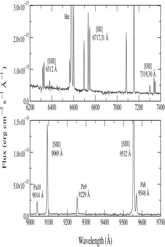
Figure 1: Spectra of IIZw40 in the two observed ranges

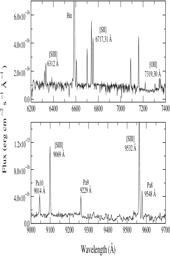
Figure 2: Spectra of UM461 in the two observed ranges

3.1 Emission lines intensities

The measurement of the emission line fluxes was made using the SPLOT routine, that integrates the line intensity over a local-fitted continuum. The errors in the line fluxes have been calculated from the expression $\sigma_{l}$ = $\sigma_{c}$N^1/2[1 + EW/(N$\Delta$)]^1/2, where $\sigma_{l}$ is the error in the line flux, $\sigma_{c}$ represents the standard deviation in a box near the measured emission line and stands for the error in the continuum placement, N is the number of pixels used in the measurement of the line flux, EW is the line equivalent width, and $\Delta$ is the wavelength dispersion in angstroms per pixel.

We have not attempted to quantify the amount of internal reddening, but have rather decided to measure each line intensity relative to that of the nearest hydrogen recombination line which, in turn, has been taken to be equal to its theoretical Case B recombination value (e.g. Osterbrock 1989) at the electron temperature estimated from the observed [OIII] lines ratio. This procedure also minimizes any possible error introduced by the flux-calibration. Only the [OII] $\lambda\lambda$ 7319, 7330 Å line intensities have been corrected for reddening for which published values of the reddening constant C(H$\beta$) have been used. In the cases in which the [SIII] $\lambda$ 9532 Å line could not be measured with the required level of confidence due to poor water absorption corrections, only the [SIII] $\lambda$ 9069 Å line was used and a ratio between the two lines of 2.44 was assumed.

Our measured emission line intensities relative to H$\beta$ = 100, are given in Table 3 together with data on the blue and visible spectral ranges taken from the literature. For most of the objects, the comparison of the intensities of the emission lines in the overlapping spectral region shows an acceptable agreement.

Table 3: Relative emission line intensities

$\lambda$ (Å)	0553+034 $\equiv$ II Zw 40		0635+756 $\equiv$ Mrk 5		0749+568
	GIT00	our data	IT98	our data	ITL97	our data
3727 [OII]	83.9$\pm$1.2		212.9$\pm$3.1		166.8$\pm$4.3
4072 [SII]					2.0$\pm$1.1
4363 [OIII]	10.9$\pm$0.4		4.4$\pm$0.5		9.8$\pm$1.1
4861 H$\beta$	100.0$\pm$1.0	100	100.0$\pm$1.5	100	100.0$\pm$2.7	100
4959 [OIII]	246.2$\pm$2.1		129.8$\pm$1.8		167.2$\pm$3.9
5007 [OIII]	740.9$\pm$5.6		381.5$\pm$4.5		488.0$\pm$9.9
5199 [NI]
6300 [OI]	1.6$\pm$0.1	1.23$\pm$0.04	4.3$\pm$0.3	3.4$\pm$0.2	4.1$\pm$0.8	5.3$\pm$0.2
6312 [SIII]	1.6$\pm$0.1	1.39$\pm$0.04	2.1$\pm$0.4	1.6$\pm$0.2	1.8$\pm$0.6	2.3$\pm$0.3
6363 [OI]		0.42$\pm$0.04	1.3$\pm$0.3	1.8$\pm$0.2	2.3$\pm$0.1	1.9$\pm$0.2
6548 [NII]		2.82$\pm$0.04		5.4$\pm$0.2		2.4$\pm$0.3
6563 H$\alpha$	287.2$\pm$2.4	281.0$\pm$0.9	285.7$\pm$3.7	283.0$\pm$2.6	279.7$\pm$6.4	280.0$\pm$1.7
6584 [NII]	6.3$\pm$0.2	5.8$\pm$0.1	13.8$\pm$0.5	13.7$\pm$0.2	7.6$\pm$0.7	6.8$\pm$0.1
6678 [HeI]	3.2$\pm$0.1	3.2$\pm$0.1	3.1$\pm$0.3	3.5$\pm$0.1	3.9$\pm$0.8	2.7$\pm$0.1
6717 [SII]	6.7$\pm$0.2	6.09$\pm$0.08	23.3$\pm$0.6	21.9$\pm$0.1	17.8$\pm$1.1	13.3$\pm$0.1
6731 [SII]	5.4$\pm$0.1	5.17$\pm$0.08	16.6$\pm$0.5	15.7$\pm$0.1	11.4$\pm$0.8	10.1$\pm$0.2
7065 [HeI]	4.2$\pm$0.1	4.9$\pm$0.1	2.5$\pm$0.2	2.1$\pm$0.1	2.4$\pm$0.5	2.2$\pm$0.2
7137 [ArIII]	7.7$\pm$0.1	9.1$\pm$0.1	8.7$\pm$0.3	8.7$\pm$0.2	6.5$\pm$0.7	5.1$\pm$0.1
7319 [OII]		1.57$\pm$0.08		2.9$\pm$0.2	3.1$\pm$0.6	1.9$\pm$0.1
7330 [OII]		1.30$\pm$0.08		2.7$\pm$0.2	1.8$\pm$0.4	1.5$\pm$0.1
9014 Pa10		1.8$\pm$0.1		1.8$\pm$0.1		1.8$\pm$0.2
9069 [SIII]		13.9$\pm$0.6		15.9$\pm$1.2		12.7$\pm$1.4
9532 [SIII]		27.9$\pm$1.0		32.2$\pm$2.2
9548 Pa8		3.5$\pm$0.1		3.6$\pm$0.2
C(H$\beta$)	0.09		0.42		0.12

Table 3: Continued

$\lambda$ (Å)	0926+606		0946+171 $\equiv$ Mrk 709		0946+558 $\equiv$ Mrk 22
	ITL97	our data	T91	our data	ITL94	our data
3727 [OII]	178.5$\pm$1.2		183.6$\pm$18.1		148.7$\pm$2.3
4072 [SII]	2.6$\pm$0.4				1.5$\pm$0.3
4363 [OIII]	8.3$\pm$0.3		8.8$\pm$0.5		8.2$\pm$0.3
4861 H$\beta$	100.0$\pm$0.7	100	100	100	100.0$\pm$1.1	100
4959 [OIII]	162.8$\pm$1.0		121.5$\pm$0.9		182.4$\pm$1.6
5007 [OIII]	477.2$\pm$2.6		369.6$\pm$4.2		545.5$\pm$4.2
5199 [NI]	0.7$\pm$0.2				0.3$\pm$0.1
6300 [OI]	3.6$\pm$0.2	3.6$\pm$0.2		7.3$\pm$0.1	1.9$\pm$0.1	1.7$\pm$0.1
6312 [SIII]	1.9$\pm$0.2	2.0$\pm$0.1		1.4$\pm$0.1	2.4$\pm$0.1	3.0$\pm$0.1
6363 [OI]	1.1$\pm$0.2	1.4$\pm$0.1		2.5$\pm$0.2	0.6$\pm$0.1	1.1$\pm$0.3
6548 [NII]		3.3$\pm$0.2		8.5$\pm$0.1		2.6$\pm$0.3
6563 H$\alpha$	280.4$\pm$1.7	282.0$\pm$0.7	286.0$\pm$ 1.0	281.0$\pm$0.7	282.5$\pm$2.5	283.0$\pm$1.3
6584 [NII]	8.3$\pm$0.4	9.3$\pm$0.4	27.9$\pm$2.2	34.2$\pm$0.2	6.4$\pm$0.2	8.0$\pm$0.1
6678 [HeI]	3.0$\pm$0.2	3.3$\pm$0.4		3.1$\pm$0.2	2.9$\pm$0.2	3.4$\pm$0.1
6717 [SII]	18.2$\pm$0.3	18.7$\pm$0.3	31.3$\pm$3.0	36.2$\pm$0.2	11.4$\pm$0.3	15.1$\pm$0.1
6731 [SII]	14.6$\pm$0.3	13.3$\pm$0.2	28.5$\pm$3.0	26.1$\pm$0.2	8.5$\pm$0.2	11.5$\pm$0.4
7065 [HeI]	2.2$\pm$0.1	2.2$\pm$0.1		2.1$\pm$0.1	2.4$\pm$0.2	2.7$\pm$0.3
7137 [ArIII]	6.6$\pm$0.2	7.4$\pm$0.1		8.0$\pm$0.1	6.5$\pm$0.2	6.8$\pm$0.2
7319 [OII]	2.6$\pm$0.2	2.2$\pm$0.1		2.9$\pm$0.1	1.6$\pm$0.2	1.0$\pm$0.2
7330 [OII]	2.0$\pm$0.1	2.1$\pm$0.1		2.8$\pm$0.1	2.0$\pm$0.2	1.6$\pm$0.1
9014 Pa10		1.8$\pm$0.1		1.8$\pm$0.1		1.8$\pm$0.3
9069 [SIII]		12.2$\pm$1.2		8.7$\pm$1.0		14.8$\pm$2.0
9532 [SIII]		36.0$\pm$4.6
9548 Pa8		3.5$\pm$0.1
C(H$\beta$)	0.29		0-0.22		0.18

Table 3: Continued

$\lambda$ (Å)	1030+583 $\equiv$ Mrk 1434		1102+294 $\equiv$ Mrk 36		1124+792 $\equiv$ VII Zw 403
	ITL97	our data	IT98	our data	ITL97	our data
3727 [OII]	96.8$\pm$0.6		129.3$\pm$1.5		133.3$\pm$0.9
4072 [SII]	1.8$\pm$0.3		1.6$\pm$0.5		1.3$\pm$0.4
4363 [OIII]	10.4$\pm$0.2		9.6$\pm$0.5		7.1$\pm$0.2
4861 H$\beta$	100.0$\pm$0.6	100	100.0$\pm$1.1	100	100.0$\pm$0.7	100
4959 [OIII]	170.4$\pm$0.8		162.2$\pm$1.6		114.3$\pm$0.8
5007 [OIII]	502.8$\pm$2.1		483.4$\pm$4.2		345.5$\pm$3.9
5199 [NI]	0.8$\pm$0.2
6300 [OI]	2.6$\pm$0.2	1.4$\pm$0.1	2.8$\pm$0.3	2.0$\pm$0.2	1.9$\pm$0.1
6312 [SIII]	1.8$\pm$0.1	1.6$\pm$0.1	1.8$\pm$0.3	1.8$\pm$0.2	1.3$\pm$0.1	1.3$\pm$0.1
6363 [OI]	0.6$\pm$0.1	0.7$\pm$0.1	1.2$\pm$0.2	0.9$\pm$0.2	1.3$\pm$0.1
6548 [NII]		1.4$\pm$0.2		1.7$\pm$0.1		1.9$\pm$0.3
6563 H$\alpha$	278.6$\pm$1.3	281.0$\pm$0.3	279.1$\pm$2.7	281.0$\pm$0.9	278.7$\pm$1.6	281.0$\pm$0.9
6584 [NII]	3.1$\pm$0.1	3.9$\pm$0.3	5.3$\pm$0.3	4.9$\pm$1.2	5.0$\pm$0.2	4.2$\pm$0.2
6678 [HeI]	2.8$\pm$0.1	2.7$\pm$0.1	2.7$\pm$0.3	2.6$\pm$0.1	2.9$\pm$0.1	2.9$\pm$0.1
6717 [SII]	9.6$\pm$0.2	9.04$\pm$0.08	11.7$\pm$0.4	11.4$\pm$0.1	10.3$\pm$0.2	7.7$\pm$0.1
6731 [SII]	6.7$\pm$0.1	6.03$\pm$0.08	8.4$\pm$0.4	8.6$\pm$0.1	7.5$\pm$0.2	5.3$\pm$0.1
7065 [HeI]	2.3$\pm$0.1	2.1$\pm$0.1	2.5$\pm$0.3	2.1$\pm$0.2	2.0$\pm$0.1
7137 [ArIII]	6.0$\pm$0.1	4.8$\pm$0.1	6.2$\pm$0.3	5.4$\pm$0.2	6.4$\pm$0.2	5.5$\pm$0.1
7319 [OII]	1.8$\pm$0.2	1.3$\pm$0.1		2.3$\pm$0.2	2.3$\pm$0.2	1.3$\pm$0.1
7330 [OII]	1.0$\pm$0.1	1.0$\pm$0.1		1.6$\pm$0.2	1.5$\pm$0.2	0.9$\pm$0.1
9014 Pa10		1.8$\pm$0.3		1.8$\pm$0.1		1.8$\pm$0.2
9069 [SIII]		9.2$\pm$0.8		11.9$\pm$1.4		11.7$\pm$1.3
9532 [SIII]				29.5$\pm$3.5
9548 Pa8				3.5$\pm$0.4
C(H$\beta$)	0.00		0.02		0.00

Table 3: Continued

$\lambda$ (Å)	1148-020 $\equiv$ UM 461		1150-021 $\equiv$ UM 462		1223+487 $\equiv$ Mrk 209
	IT98	our data	IT98	our data	ITL97	our data
3727 [OII]	52.7$\pm$1.5		174.2$\pm$1.0		71.9$\pm$0.2
4072 [SII]			2.2$\pm$0.4		1.2$\pm$0.1
4363 [OIII]	13.6$\pm$0.7		7.8$\pm$0.2		12.7$\pm$0.1
4861 H$\beta$	100.0$\pm$2.0	100	100.0$\pm$0.6	100	100.0$\pm$0.2	100
4959 [OIII]	203.9$\pm$3.4		166.3$\pm$0.9		196.0$\pm$0.3
5007 [OIII]	602.2$\pm$9.0		492.9$\pm$2.3		554.3$\pm$0.8
5199 [NI]					0.3$\pm$0.1
6300 [OI]	1.9$\pm$0.4	1.7$\pm$0.1	3.8$\pm$0.2	3.5$\pm$0.2	1.4$\pm$0.1	1.6$\pm$0.2
6312 [SIII]	1.2$\pm$0.4	2.0$\pm$0.1	1.9$\pm$0.1	2.1$\pm$0.2	1.7$\pm$0.1	1.9$\pm$0.1
6363 [OI]			1.2$\pm$0.1	1.1$\pm$0.1	0.5$\pm$0.1
6548 [NII]				3.5$\pm$0.3		1.6$\pm$0.2
6563 H$\alpha$	278.4$\pm$4.8	280.0$\pm$0.7	282.6$\pm$1.5	282.0$\pm$0.6	277.7$\pm$0.5	280.0$\pm$0.1
6584 [NII]	2.1$\pm$0.4	2.8$\pm$0.2	7.3$\pm$0.2	7.3$\pm$0.2	2.9$\pm$0.1	3.6$\pm$0.1
6678 [HeI]	2.9$\pm$0.3	3.2$\pm$0.1	3.0$\pm$0.1	3.0$\pm$0.1	2.9$\pm$0.1	3.3$\pm$0.2
6717 [SII]	5.2$\pm$0.4	5.8$\pm$0.1	16.8$\pm$0.2	16.2$\pm$0.3	6.1$\pm$0.1	5.9$\pm$0.2
6731 [SII]	4.2$\pm$0.4	4.5$\pm$0.1	11.2$\pm$0.2	12.1$\pm$0.2	4.5$\pm$0.1	4.7$\pm$0.2
7065 [HeI]	2.8$\pm$0.3	2.7$\pm$0.1	3.0$\pm$0.1	2.0$\pm$0.1	2.4$\pm$0.1	2.2$\pm$0.1
7137 [ArIII]	4.6$\pm$0.4	4.8$\pm$0.1	8.5$\pm$0.1	5.7$\pm$0.1	5.9$\pm$0.1	5.5$\pm$0.1
7319 [OII]		1.0$\pm$0.1		2.34$\pm$0.06	1.1$\pm$0.1	0.9$\pm$0.1
7330 [OII]		1.1$\pm$0.1		1.96$\pm$0.09	1.0$\pm$0.1	0.8$\pm$0.1
9014 Pa10		1.8$\pm$0.2		1.8$\pm$0.2		1.8$\pm$0.1
9069 [SIII]		12.4$\pm$0.8		10.5$\pm$1.5		12.2$\pm$1.2
9532 [SIII]		21.7$\pm$ 0.7		35.0$\pm$3.6
9548 Pa8		3.5$\pm$0.3		3.5$\pm$0.4
C(H$\beta$)	0.12		0.29		0.00

3.2 Line temperatures, number densities and ionic abundances

Electron densities were determined from the [SII] $\lambda$6717 Å/$\lambda$6731 Å ratio using a five-level statistical equilibrium model (De Robertis, Dufour & Hunt 1987; Shaw & Dufour 1995). Except in IIZw40, with a value 290 $cm^{-3}$, the diagnostic ratios give low values of the density.

For all the objects we have derived the value of t([SIII]), from the ($\lambda$9069Å+$\lambda$9532Å)/$\lambda$6312Å ratio. Besides, we have determined t([OII]), from the ratio of $\lambda$3727Å/($\lambda$7319Å+$\lambda$7330Å), by combining, in most cases, our data in the red with complementary data in the blue taken from the literature (see Table 3). The same sources of data have been used to derive t([OIII]), from the ratio of ($\lambda$4959Å+$\lambda$5007Å)/$\lambda$4363Å and, for 7 objects of the sample, t([SII]) from the ratio $\lambda$(6717Å+$\lambda$6731Å)/$\lambda$4072Å. In the cases in which the agreement between our measured line intensities and those in the literature is shown to be good, the values with the smaller observational errors have been used to derive a given line temperature. Otherwise we have preferred to use the line intensities corresponding to the same data source. In all cases, line temperatures were derived from the corresponding line ratios using the five-level atom code, assuming in each case the electron density deduced from the [SII] line ratio and using the most recent atomic collision strength data as listed in Table 4.

The [OII] $\lambda$7319Å+$\lambda$7330Å lines as well as the [SII]$\lambda$$\lambda$ 4068, 4074 Å lines can have a contribution by direct recombination which increases with temperature. We have estimated these contributions using the calculated [OIII] electron temperatures to be less than 4 % for the [OII] lines and less than 0.01 % for the [SII] lines in all cases and therefore we have not corrected for this effect.

Table 4: Sources of the effective collision strengths of each ion

Ion	References
$[OII]$	McLaughlin & Bell, 1998
$[OIII]$,$[NII]$	Lennon & Burke, 1994
$[SII]$	Ramsbotton, Bell & Stafford, 1996
$[SIII]$	Tayal & Gupta, 1999

For all the observed galaxies, at least three line temperatures have been derived. Electron densities and line temperatures, with their corresponding errors, for each of the observed galaxies are given in Table 5.

Table 5: Physical properties of the observed galaxies

Object	II Zw 40	Mrk 5	0749+568	0926+606	Mrk 709	Mrk 22
$\log U$	-2.23$\pm$0.08	-2.6$\pm$0.2	-2.55$\pm$0.10	-2.6$\pm$0.1	-2.6$\pm$0.1	-2.45$\pm$0.10
$n_{e}$([SII])	290$\pm$60	20$\pm$10	100$\pm$50	$\leq$50	$\leq$30	110$\pm$80
$t_{e}$([OII])	1.27$\pm$0.06	1.32$\pm$0.08	1.38$\pm$0.12	1.23$\pm$0.04	1.50$\pm$0.16	1.16$\pm$0.09
$t_{e}$([OIII])	1.34$\pm$0.03	1.22$\pm$0.06	1.54$\pm$0.10	1.43$\pm$0.03	1.67$\pm$0.06	1.35$\pm$0.03
$t_{e}$([SII])	–	–	–	1.04$\pm$0.14	–	0.96$\pm$0.16
$t_{e}$([SIII])	1.30$\pm$0.05	1.33$\pm$0.15	1.86$\pm$0.36	1.52$\pm$0.18	1.65$\pm$0.23	1.98$\pm$0.28
$O^{+}/H^{+}$ $(\times 10^{4})$	0.12$\pm$0.02	0.28$\pm$0.07	0.19$\pm$0.17	0.29$\pm$0.04	0.16$\pm$0.08	0.31$\pm$0.11
$O^{2+}/H^{+}$ $(\times 10^{4})$	1.08$\pm$0.08	0.73$\pm$0.12	0.51$\pm$0.10	0.59$\pm$0.04	0.31$\pm$0.03	0.78$\pm$0.05
$12+\log(O/H)$	8.08$\pm$0.03	8.00$\pm$0.08	7.84$\pm$0.09	7.95$\pm$0.04	7.68$\pm$0.09	8.04$\pm$0.06
$S^{+}/H^{+}$ $(\times 10^{6})$	0.15$\pm$0.02	0.48$\pm$0.06	0.27$\pm$0.05	0.68$\pm$0.27	0.62$\pm$0.13	0.71$\pm$0.40
$S^{2+}/H^{+}$ $(\times 10^{6})$	0.94$\pm$0.09	1.06$\pm$0.27	0.66$\pm$0.25	0.89$\pm$0.27	0.50$\pm$0.16	0.71$\pm$0.23
$\log(N^{+}/O^{+})$	-1.31$\pm$0.05	-1.29$\pm$0.05	-1.48$\pm$0.08	-1.44$\pm$0.04	-0.82$\pm$0.09	-1.47$\pm$0.07
$N^{+}/H^{+}$ $(\times 10^{6})$	0.59$\pm$0.06	1.24$\pm$0.15	0.56$\pm$0.10	0.91$\pm$0.09	2.33$\pm$0.39	0.84$\pm$0.15
$12+\log(N/H)$	6.77$\pm$0.07	6.71$\pm$0.12	6.36$\pm$0.17	6.51$\pm$0.08	6.86$\pm$0.08	6.57$\pm$0.13

Table 5: Continued

Object	Mrk 1434	Mrk 36	VII Zw 403	UM 461	UM 462	Mrk 209
$\log U$	-2.4$\pm$0.1	-2.65$\pm$0.20	-2.6$\pm$0.1	-2.1$\pm$0.1	-2.6$\pm$0.1	-2.3$\pm$0.1
$n_{e}$([SII])	$\leq$10	90$\pm$40	$\leq$10	140$\pm$70	80$\pm$60	190$\pm$140
$t_{e}$([OII])	1.24$\pm$0.08	1.37$\pm$0.12	1.42$\pm$0.12	1.64$\pm$0.18	1.19$\pm$0.03	1.22$\pm$0.08
$t_{e}$([OIII])	1.55$\pm$0.02	1.53$\pm$0.05	1.52$\pm$0.03	1.62$\pm$0.05	1.38$\pm$0.02	1.62$\pm$0.01
$t_{e}$([SII])	1.54$\pm$0.32	1.09$\pm$0.28	1.05$\pm$0.27	–	1.00$\pm$0.15	1.25$\pm$0.13
$t_{e}$([SIII])	1.73$\pm$0.20	1.62$\pm$0.30	1.30$\pm$0.14	1.95$\pm$0.16	1.66$\pm$0.25	1.60$\pm$0.17
$O^{+}/H^{+}$ $(\times 10^{4})$	0.16$\pm$0.04	0.15$\pm$0.05	0.14$\pm$0.04	0.04$\pm$0.01	0.32$\pm$0.03	0.12$\pm$0.03
$O^{2+}/H^{+}$ $(\times 10^{4})$	0.51$\pm$0.02	0.50$\pm$0.05	0.36$\pm$0.02	0.55$\pm$0.05	0.66$\pm$0.03	0.51$\pm$0.01
12+log(O/H)	7.82$\pm$0.04	7.82$\pm$0.06	7.70$\pm$0.05	7.77$\pm$0.05	8.00$\pm$0.03	7.80$\pm$0.03
$S^{+}/H^{+}$ $(\times 10^{6})$	0.15$\pm$0.07	0.43$\pm$0.37	0.30$\pm$0.28	0.09$\pm$0.02	0.67$\pm$0.32	0.15$\pm$0.04
$S^{2+}/H^{+}$ $(\times 10^{6})$	0.51$\pm$0.12	0.72$\pm$0.29	0.92$\pm$0.28	0.47$\pm$0.06	0.76$\pm$0.25	0.73$\pm$0.18
$\log(N^{+}/O^{+})$	-1.55$\pm$0.08	-1.52$\pm$0.07	-1.55$\pm$0.08	-1.27$\pm$0.09	-1.51$\pm$0.09	-1.48$\pm$0.06
$N/H^{+}$ $(\times 10^{6})$	0.38$\pm$0.08	0.38$\pm$0.15	0.36$\pm$0.08	0.18$\pm$0.05	.0.82$\pm$0.17	0.38$\pm$0.07
$12+\log(N/H)$	6.28$\pm$0.12	6.29$\pm$0.13	6.15$\pm$0.13	6.49$\pm$0.14	6.48$\pm$0.06	6.37$\pm$0.09

We have calculated the ionic abundances of $O^{+}$, $O^{2+}$, $S^{+}$, $S^{2+}$ and $N^{+}$ using standard expressions (Pagel et al. 1992), and using for each ion its corresponding line temperature, except for [SII] in the objects for which no measurements of the [SII] $\lambda\lambda$4068,4076 Å lines exist, and [NII] for which no measurements of the [NII]$\lambda$ 5755 Å are reported. In theses cases, under the assumption of a homogeneus electron temperature in the low excitation zone, we have taken the aproximation of t([NII])$\approx$t([SII])$\approx$t([OII]). The computed ionic abundances relative to H⁺ are also shown in Table 5.

3.3 Ionisation correction factors and photo-ionisation models

In order to derive the total chemical abundances we must add the contribution of unseen stages of ionisation and this requires the reconstruction of the ionisation structure of the region which, in turn, allows the determination of appropriate ionisation correction factors (ICF). To this purpose we have modelled each HII galaxy using the recent version of the photo-ionisation code CLOUDY (Ferland 2002). Each modelled galaxy has been characterized by a set of input parameters including chemical abundances, ionising continuum and nebular geometry in a very simple way: the galaxy has been assumed to be spherically symmetric with the ionised emmitting gas, assumed to be of constant density, located at a distance very large compared to its thickness, therefore resulting in a plane-parallel geometry. Its degree of ionisation of the gas has been specified in terms of the ionisation parameter U, the ratio of the ionising photon density to the particle density. This can be estimated from suitable line ratios. At low metallicities, as the ones expected for HII galaxies, the use of the sum of the [SII] lines at $\lambda\lambda$ 6717,6731 Å can be used (e.g. García-Vargas, Bressan & Díaz 1995).

The nebula has been assumed to be ionised by a source represented by a single star whose effective temperature has been estimated from the $R_{23}$ and $R_{33}$ parameters as described in Cerviño & Mas-Hesse (1994) and whose spectral energy distribution has been taken from the CoStar NLTE single-star stellar atmosphere models (Schaerer and de Koter 1997) of 0.2 times the solar metallicity. Finally, as input abundances we have used the sum of the respective ionic abundances for O and S, the N/O ratio as given by the N⁺/O⁺ ratio and the rest of heavy elements scaled to oxygen in solar proportions as given by Grevesse & Sauval (1998). The refractory elements: Fe, Mg, Al, Ca, Na, Ni have been depleted by a factor of 10, and Si by a factor of 2 (Garnett et al. 1995), to take into account the presence of dust grains. With these imput parametrers we have calculated a first photo-ionisation model which has then been optimized.

The predicted line intensities for the best fitting models, together with the resulting functional parameters: U, T_eff and chemical abundances are given in Table 6 in comparison with observations. Also listed are the ICF for S and N as well as their total abundance values.

Table 6: Comparison between observations (Obs.) and results from photo-ionisation models, as described in the text.

	II Zw 40		Mrk 5		0749+568
	Obs.	Model	Obs.	Model	Obs.	Model
$\log U$	-2.23$\pm$0.08	-2.23	-2.6$\pm$0.2	-2.85	-2.55$\pm$0.10	-2.71
$T_{eff}(K)$	–	47300	–	50100	–	50400
3727 [OII]	83.9$\pm$1.2	84.5	212.9$\pm$3.1	197.1	166.8$\pm$4.3	157.9
4363 [OIII]	10.9$\pm$0.4	10.4	4.4$\pm$0.5	5.2	9.8$\pm$1.1	6.8
4959 [OIII]	246.2$\pm$2.1	248.1	129.8$\pm$1.8	126.5	167.2$\pm$3.9	153.2
5007 [OIII]	740.9$\pm$5.6	746.7	381.5$\pm$4.5	380.7	488.0$\pm$9.9	461.3
6312 [SIII]	1.4$\pm$0.04	1.9	1.6$\pm$0.2	1.6	2.3$\pm$0.3	1.1
6720 [SII]	11.3$\pm$0.2	11.9	37.6$\pm$0.2	28.2	23.4$\pm$0.3	14.1
7325 [OII]	2.9$\pm$0.1	3.3	5.6$\pm$0.4	4.5	3.4$\pm$0.2	5.0
9069 [SIII]	13.9$\pm$0.6	17.0	15.9$\pm$1.2	14.1	12.7$\pm$1.4	9.1
9532 [SIII]	27.9$\pm$1.0	42.2	32.2$\pm$2.2	34.9	–	22.5
t([OII])	1.27$\pm$0.06	1.39	1.31$\pm$0.08	1.37	1.38$\pm$0.12	1.38
t([OIII])	1.34$\pm$0.03	1.31	1.22$\pm$0.06	1.30	1.54$\pm$0.10	1.34
t([SIII])	1.30$\pm$0.05	1.29	1.33$\pm$0.16	1.28	1.86$\pm$0.36	1.32
12+log(O+/H+)	7.08$\pm$0.07	7.15	7.45$\pm$0.10	7.45	7.28$\pm$0.28	7.34
12+log(O2+/H+)	8.03$\pm$0.03	8.04	7.86$\pm$0.07	7.67	7.71$\pm$0.08	7.75
12+log(O/H)	8.08$\pm$0.03	8.09	8.00$\pm$0.07	7.88	7.85$\pm$0.14	7.89
12+log(N+/H+)	5.77$\pm$0.04	5.85	6.09$\pm$0.05	6.26	5.75$\pm$ 0.07	5.76
ICF(N+)	–	9.13	–	3.04	–	3.90
12+log(N/H)	6.73$\pm$0.04	6.81	6.58$\pm$0.05	6.75	6.34$\pm$0.07	6.35
log(O+/N+)	1.31$\pm$0.04	1.29	1.29$\pm$0.05	1.19	1.48$\pm$0.08	1.59
12+log(S+/H+)	5.18$\pm$0.05	5.38	5.68$\pm$0.19	5.77	5.43$\pm$ 0.07	5.41
12+log(S2+/H+)	5.97$\pm$0.04	6.18	6.03$\pm$0.03	6.03	5.82$\pm$0.14	5.79
12+log($S^{+}+S^{2+}$/H+)	5.97$\pm$0.04	6.24	6.19$\pm$0.09	6.22	5.97$\pm$0.12	5.94
ICF(S++S2+)	–	1.24	–	0.86	–	0.92
ICF(S+)	–	9.09	–	2.41	–	3.09
12+log(S/H)	6.13$\pm$0.04	6.36	6.12$\pm$0.13	6.24	5.93$\pm$0.12	5.97

Table 6: Continued

	0926+606		Mrk 709		Mrk 22
	Obs.	Model	Obs.	Model	Obs.	Model
$\log U$	-2.6$\pm$0.1	-2.72	-2.6$\pm$0.1	-2.81	-2.45$\pm$0.10	-2.59
$T_{eff}$	–	50200	–	49400	–	48700
3727 [OII]	178.5$\pm$4.2	171.3	183.6$\pm$18.1	182.0	148.7$\pm$2.3	145.9
4363 [OIII]	8.3$\pm$0.3	6.4	8.8$\pm$0.5	5.4	8.2$\pm$0.3	7.5
4959 [OIII]	162.8$\pm$1.0	153.2	121.5$\pm$0.9	129.9	182.4$\pm$1.6	179.4
5007 [OIII]	477.2$\pm$2.6	461.1	369.6$\pm$4.2	391.1	545.5$\pm$4.2	539.9
6312 [SIII]	2.0$\pm$0.1	1.7	1.4$\pm$0.1	1.4	3.0$\pm$0.1	1.6
6720 [SII]	32.0$\pm$0.5	24.3	62.3$\pm$0.4	23.7	26.6$\pm$0.5	18.9
7325 [OII]	4.3$\pm$0.2	4.8	5.7$\pm$0.2	5.2	2.6$\pm$0.3	4.6
9069 [SIII]	12.2$\pm$1.7	15.0	8.7$\pm$1.0	12.7	14.8$\pm$2.0	14.4
9532 [SIII]	36.0$\pm$4.6	37.1	–	31.5	–	35.7
t([OII])	1.23$\pm$0.04	1.37	1.50$\pm$0.16	1.39	1.16$\pm$0.09	1.36
t([OIII])	1.43$\pm$0.03	1.31	1.67$\pm$0.06	1.31	1.35$\pm$0.03	1.31
t([SIII])	1.52$\pm$0.18	1.29	1.65$\pm$0.23	1.29	1.98$\pm$0.28	1.29
12+log(O+/H+)	7.46$\pm$0.06	7.40	7.20$\pm$0.18	7.41	7.49$\pm$0.13	7.34
12+log(O2+/H+)	7.77$\pm$0.03	7.77	7.49$\pm$0.04	7.68	7.89$\pm$0.03	7.86
12+log(O/H)	7.94$\pm$0.04	7.92	7.68$\pm$0.05	7.87	8.04$\pm$0.06	7.98
12+log(N+/H+)	5.96$\pm$0.04	5.88	6.37$\pm$0.07	6.45	5.92$\pm$0.07	5.85
ICF(N+)	–	3.80	–	3.26	–	4.56
12+log(N/H)	6.54$\pm$0.04	6.46	6.88$\pm$0.07	6.96	6.58$\pm$0.07	6.51
log(O+/N+)	1.43$\pm$0.04	1.52	0.81$\pm$0.03	0.97	1.47$\pm$0.07	1.49
12+log(S+/H+)	5.83$\pm$0.15	5.71	5.79$\pm$0.03	5.64	5.85$\pm$0.19	5.60
12+log(S2+/H+)	5.95$\pm$0.12	6.07	5.71$\pm$0.01	5.93	5.85$\pm$0.12	6.08
12+log($S^{+}+S^{2+}$/H+)	6.20$\pm$0.13	6.23	6.05$\pm$0.07	6.11	6.15$\pm$0.16	6.12
ICF(S++S2+)	–	0.92	–	0.87	–	0.99
ICF(S+)	–	3.04	–	2.58	–	3.92
12+log(S/H)	6.16$\pm$0.13	6.26	5.99$\pm$0.02	6.14	6.15$\pm$0.16	6.25

Table 6: Continued

	Mrk 1434		Mrk 36		VII Zw 403
	Obs.	Model	Obs.	Model	Obs.	Model
$\log U$	-2.4$\pm$0.1	-2.36	-2.65$\pm$0.20	-2.51	-2.6 $\pm$0.1	-2.62
$T_{eff}$	–	46000	–	42300	–	42500
3727 [OII]	96.8$\pm$0.6	97.3	129.3$\pm$1.5	124.1	133.3$\pm$0.9	132.3
4363 [OIII]	10.4$\pm$0.2	7.7	9.6$\pm$0.5	6.9	7.1$\pm$0.2	4.4
4959 [OIII]	170.4$\pm$0.8	171.7	162.2$\pm$1.6	170.7	114.3$\pm$0.8	117.0
5007 [OIII]	502.8$\pm$2.1	516.9	483.4$\pm$4.2	513.7	345.5$\pm$3.9	352.0
6312 [SIII]	1.6$\pm$0.1	0.8	1.8$\pm$0.2	1.8	1.3$\pm$0.1	1.3
6720 [SII]	15.1$\pm$0.2	6.8	20.0$\pm$0.2	19.6	13.0$\pm$0.2	14.4
7325 [OII]	2.3$\pm$0.2	2.7	3.9$\pm$0.4	3.8	2.2$\pm$0.2	3.5
9069 [SIII]	9.2$\pm$0.8	6.9	11.9$\pm$0.4	16.6	11.7$\pm$1.3	11.9
9532 [SIII]	–	17.1	29.5$\pm$3.5	41.2	–	29.4
t([OII])	1.24$\pm$0.08	1.38	1.37$\pm$0.12	1.37	1.41$\pm$0.12	1.33
t([OIII])	1.55$\pm$0.02	1.34	1.53$\pm$0.05	1.29	1.52$\pm$0.03	1.25
t([SIII])	1.73$\pm$0.20	1.32	1.62$\pm$0.30	1.27	1.30$\pm$0.14	1.24
12+log(O+/H+)	7.20$\pm$0.10	7.00	7.18$\pm$0.12	7.28	7.15$\pm$0.11	7.32
12+log(O2+/H+)	7.71$\pm$0.02	7.70	7.70$\pm$0.04	7.87	7.56$\pm$0.02	7.73
12+log(O/H)	7.83$\pm$0.04	7.78	7.81$\pm$0.06	7.97	7.70$\pm$0.05	7.88
12+log(N+/H+)	5.58$\pm$0.08	5.38	5.58$\pm$0.14	5.59	5.56$\pm$0.09	5.58
ICF(N+)	–	6.96	–	5.23	–	4.24
12+log(N/H)	6.42$\pm$0.08	6.22	6.30$\pm$0.14	6.31	6.18$\pm$0.09	6.21
log(O+/N+)	1.58$\pm$0.08	1.62	1.52$\pm$0.07	1.68	1.56$\pm$0.08	1.74
12+log(S+/H+)	5.18$\pm$0.17	5.15	5.63$\pm$0.27	5.63	5.48$\pm$0.29	5.51
12+log(S2+/H+)	5.71$\pm$0.09	5.76	5.86$\pm$0.15	6.16	5.96$\pm$0.12	6.02
12+log($S^{+}+S^{2+}$/H+)	5.82$\pm$0.11	5.85	6.06$\pm$0.20	6.00	6.09$\pm$0.16	6.13
ICF(S++S2+)	–	1.07	–	1.01	–	0.95
ICF(S+)	–	5.43	–	4.37	–	4.02
12+log(S/H)	5.85$\pm$0.11	5.92	6.07$\pm$0.20	6.32	6.06$\pm$0.16	6.16

Table 6: Continued

	UM 461		UM 462		Mrk 209
	Obs.	Model	Obs.	Model	Obs.	Model
$\log U$	-2.1$\pm$0.1	-2.15	-2.6$\pm$0.1	-2.65	-2.3$\pm$0.1	-2.29
$T_{eff}$	–	46600	–	48000	–	43200
3727 [OII]	52.7$\pm$1.5	57.7	174.2$\pm$1.0	170.0	71.9$\pm$0.2	68.7
4363 [OIII]	13.6$\pm$1.7	11.3	7.8$\pm$0.2	7.5	12.7$\pm$0.1	9.6
4959 [OIII]	203.9$\pm$3.4	208.8	166.3$\pm$0.9	173.1	196.0$\pm$0.3	200.8
5007 [OIII]	602.2$\pm$9.0	628.4	492.9$\pm$2.3	521.0	554.3$\pm$0.8	604.4
6312 [SIII]	2.0$\pm$0.1	0.8	2.1$\pm$0.2	2.0	1.7$\pm$0.1	1.1
6720 [SII]	10.3$\pm$0.2	4.4	28.3$\pm$0.5	24.0	10.6$\pm$0.4	6.8
7325 [OII]	2.1$\pm$0.2	1.9	4.3$\pm$0.2	5.3	1.7$\pm$0.2	2.4
9069 [SIII]	12.4$\pm$0.8	6.2	10.5$\pm$1.5	17.1	12.2$\pm$1.2	8.7
9532 [SIII]	21.7$\pm$0.7	15.3	35.0$\pm$3.6	42.5	–	21.7
t([OII])	1.66$\pm$0.19	1.49	1.19$\pm$0.03	1.38	1.23$\pm$0.08	1.40
t([OIII])	1.62$\pm$0.05	1.46	1.38$\pm$0.02	1.33	1.62$\pm$0.01	1.38
t([SIII])	1.95$\pm$0.16	1.43	1.66$\pm$0.25	1.31	1.60$\pm$0.17	1.36
12+log(O+/H+)	6.60$\pm$0.10	6.85	7.51$\pm$0.04	7.36	7.08$\pm$0.10	7.00
12+log(O2+/H+)	7.74$\pm$0.04	7.85	7.82$\pm$0.02	7.83	7.71$\pm$0.01	7.89
12+log(O/H)	7.77$\pm$0.04	7.89	7.99$\pm$0.03	7.95	7.80$\pm$0.03	7.94
12+log(N+/H+)	5.26$\pm$0.11	5.46	5.91$\pm$0.04	5.84	5.58$\pm$0.07	5.53
ICF(N+)	–	10.86	–	4.09	–	8.79
12+log(N/H)	6.29$\pm$0.11	6.50	6.53$\pm$0.04	6.45	6.52$\pm$0.07	6.48
log(O+/N+)	1.32$\pm$0.09	1.39	1.51$\pm$0.09	1.52	1.42$\pm$0.06	1.47
12+log(S+/H+)	4.95$\pm$0.09	4.90	5.83$\pm$0.17	5.65	5.18$\pm$0.10	5.15
12+log(S2+/H+)	5.67$\pm$0.05	5.68	5.88$\pm$0.12	6.14	5.86$\pm$0.10	5.86
12+log($S^{+}+S^{2+}$/H+)	5.75$\pm$0.06	5.75	6.16$\pm$0.15	6.26	5.95$\pm$0.10	5.93
ICF(S++S2+)	–	1.35	–	0.98	–	1.22
ICF(S+)	–	9.48	–	4.00	–	7.52
12+log(S/H)	5.88$\pm$0.06	5.90	6.15$\pm$0.15	6.30	6.03$\pm$0.10	6.05

4 Discussion

4.1 Line temperatures

To compute chemical abundances in ionised gas nebulae, knowledge of the electron temperature is required. Since the assumption of an isothermal gas region may not be valid due to temperature fluctuations (Peimbert 1967) and differences between the various line temperatures in each internal zone (Garnett 1992), we must use the appropriate line temperature for the calculation of the abundance of each ion. These temperatures can be deduced directly from the corresponding ratio of emission lines, but usually not all these lines are accesible in the spectra or have large associated errors. In these cases, some assumptions are usually adopted about the temperature structure through the nebula. For HII galaxies it is custommary to assume a two-zone model with a low ionisation zone where the [OII], [NII], [NeII] and [SII] lines are formed, and a high ionisation zone in which the [OIII], [NeIII] and [SIII] lines are formed; photo-ionisation models are then used to relate the temperatures representative of each zone (see, for example Pagel et al. 1992). In some cases, an intermediate zone is assumed as in Garnett (1992) for the S⁺⁺ ion.

The fact that we have been able to measure line temperatures which, in principle, correspond to these three ionisation zones, allows us to investigate to which extent these assumptions hold for the case of HII galaxies. Figure 3 shows a comparison between t([OII]) and t([SII]) for our observed objects and published data on HII galaxies for which we have derived the line temperatures in the way described in section 3.2. The 1:1 relation is shown as a dashed-dotted line. Two sequences of models of the same kind as those described in section 3.3, but with different values of the density: 10, 100 cm^-3 are also shown. Most of the data are below the 1:1 relation and are better represented, at least for our observed objects, by the sequence of models with n_e = 100 cm^-3 thus reflecting the density dependence of the two involved temperatures. However, for the whole HII galaxy sample, the average t([SII]) is still lower than predicted by models. At any rate, since for this kind of objects S²⁺ is the main contributor to the total S abundance, the commonly taken assumption of t([OII])=t([SII]) would not greatly affect the total abundance determination.

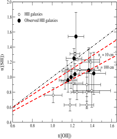
Figure 3: A comparison between the measured line temperatures of $[SII]$ and $[OII]$. Solid symbols correspond to the data in this paper. Open symbols correspond to data by Izotov et al.(1994), Izotov et al.(1997) and Izotov & Thuan (1998). The 1:1 relation is shown as a dashed-dotted line. Two sequences of models computed with electron densities of 10 and 100 cm^-3, as labelled, are also shown.

The relation between t([OII]) and t([OIII]) is shown in Figure 4. We have also added to this plot values of t([OII]) and t([OIII]) calculated from published data on HII galaxies (Izotov et al. 1994, 1997; Izotov & Thuan 1998; Guseva et al. 2000). Also shown are two relations commonly used for abundance determinations, based on photo-ionisation models from Stasińska (1980) (solid line)

$$t([OII])=0.7t([OIII])+0.3$$

and Stasińska (1990) (broken line)

$$t([OII])^{-1}=0.5(t([OIII])^{-1}+0.8)$$

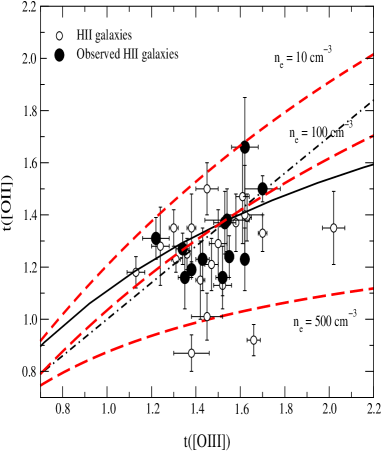
Figure 4: Comparison between the measured line temperatures of $[OIII]$ and $[OII]$. Solid symbols correspond to the data in this paper. Open symbols correspond to similar data of HII galaxies by Izotov et al.(1994), Izotov et al.(1997) and Izotov & Thuan (1998). The lines are the model-deduced relations for these line temperatures. The solid line corrresponds to the models by Stasińska (1980). The broken one corresponds to those by Stasińska (1990).

Our HII galaxies, and most of those in the literature, show t([OIII]) values between 1.2 and 1.8 and, within the errors, cluster around the model fits. The data point with the highest t([OIII]), about 2.1, shows a better agreement with the second sequence of models. There are some data points, however, that lie significantly below the theoretical relation. In this metallicity regime, large scale temperature fluctuations that would yield t([OIII]) values higher than the corresponding ion weighted mean temperature are not predicted (Garnett 1992), therefore the position of these points correspond to objects that show values of t([OII]) which are lower than predicted by the theoretical sequences. They all belong to the samples by Izotov and co-workers and correspond to: SBS0940+544N, SBS0832+699, SBS1533+574A and SBS0741+535. This latter object has a density of the order of 500 cm^-3, higher than the typical value of about 100 cm^-3. Given the density dependence of t([OII]), this could explain the position of this point in the diagram. Three sequences of models computed with different values of the density: 10, 100 and 500 cm^-3 are also shown in Fig 4 . Our model sequence for n_e = 100 cm^-3 agrees very well with the fit to the models of Stasińska (1990) and the sequence at n_e = 500 cm^-3 reproduces well the data for SBS0741+535. This explanation, however, is, in principle, not valid for the rest of the objects with low t([OII]) values for which the derived electron densities are close to the typical one. Uncertainties in reddening could also be invoked. However, in order to reconcile derived and model predicted values of t([OII]) the reddening constant should have been overestimated by an amount unplausibly large (about 1 dex). Therefore these objects require further investigation.

The adopted value of t([OII]) affects the computed ionic abundance of O⁺ and can become important in objects of relatively low excitation. For SBS0832+699, SBS1533+574A and SBS0741+535, the use of the derived t([OII]) instead of the value predicted by the Stasińska (1990) relation translates into higher O⁺/H⁺ abundances by factors of 5.2, 2.8 and 4.7 respectively and total oxygen abundances higher by 0.33, 0.21 and 0.38 dex, values much larger than the errors quoted by Izotov and co-workers (0.02, 0.03 and 0.02). Therefore, these kind of effects should be taken into account if accurate values of abundances for these objects are sought. In the absence of directly derived [OII] temperatures, higher excitation objects, where the O⁺/H⁺ fraction contributes less to the total oxygen abundance, should provide more accurate abundance determinations.

Regarding [SIII], Garnett (1992), from data on HII galaxies and GEHR, suggested that t([SIII]) is in fact intermediate between t([OII]) and t([OIII]) and provided an empirical fit:

$$t(S^{2+})=0.83t(O^{2+})+0.17$$

where t(S²⁺) and t(S²⁺) denote ion-weighted mean temperatures. The relation between both temperatures, t([OIII]) and t([SIII]) is shown in Figure 5 both for our observed galaxies and those of Garnett (1989), together with the empirical fit above. It can be seen in the figure that, although this fit works rather well when compared with the temperatures deduced directly from observations, there are non-negligible deviations that might affect the calculation of sulphur abundances in the regime of high excitation. Therefore, the validity of this relation should be further explored. It should also be taken into account that the atomic coefficients for [SIII] are suffering continuous revisions which may significantly affect the derived values of t([SIII]). This is illustrated in Table 7 where these temperatues are listed for the observed objects using different sets of coefficients.

Table 7: t([SIII]) from different sets of atomic coefficients

Refs	GMZ95	T97	TG99
II Zw 40	1.47	1.21	1.30
Mrk 5	1.51	1.26	1.33
0749+568	2.16	1.74	1.86
0926+606	1.74	1.42	1.52
Mrk 709	1.91	1.57	1.65
Mrk 22	2.32	1.85	1.98
Mrk 1434	1.97	1.61	1.73
Mrk 36	1.85	1.53	1.62
VII Zw 403	1.47	1.25	1.30
UM 461	1.98	1.84	1.95
UM 462	1.92	1.53	1.66
Mrk 209	1.84	1.52	1.60

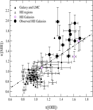
Figure 5: A comparison between the measured line temperatures of $[OIII]$ and $[SIII]$. The dark dot-dashed line is the model-deduced relation for the same ion-weighted temperatures from Garnett 1992

4.2 Ionic fractions

The fact that we can derive the ionic fractions of O, N and S allows to probe the ionisation structure of the observed nebulae and test the validity of some commonly adopted assumptions. The first of them relates to the equality of the fractions of neutral hydrogen and oxygen:

$$\frac{O^{0}}{O}=\frac{H^{0}}{H}$$

that allows to calculate O/H as:

$$\frac{O}{H}=\frac{O^{+}+O^{2+}}{H^{+}}$$

For our objects, the best fitting models yield values of O⁰/O and H⁰/H which are equal inside 95 % except for two objects: IIZw40 and Mrk209 in which the ratio deviate from unity by 20 % and 10 % respectively. These are the objects with the highest densities in our sample: 290 cm^-3 for IIZw40 and 190 cm^-3 for Mrk209. In any case, given the low proportion of neutral oxygen in these objects, the assumption above seems to be well justified.

Also the aproximation $(N/O)\approx(N^{+}/O^{+})$, seems to hold to better than 85 % and the N/O ratio, as computed using the ICFs for nitrogen from the models, equals the N⁺/O⁺ derived observationally except for one object : Mrk 5 for which this latter ratio is found to be larger by about 25 %.

The situation regarding sulphur requires further attention. Even when we observe the two major ionisation states of sulphur: S⁺ and S⁺⁺, we still have to correct for the possible presence of S³⁺ which, in the absence of IR observations of [SIV], means we have to rely on photo-ionisation models.

A first scheme for the ionisation correction necessary to calculate the total abundance of sulphur was given by Peimbert & Costero (1969) based on the similarity of the ionisation potentials of S²⁺ and O⁺. Then: S/O = (S⁺ + S⁺⁺)/O⁺ and

$$ICF(S^{+}+S^{2+})=\frac{S/H}{(S^{+}+S^{2+})/H^{+}}=\left(\frac{S}{S^{+}+S^{2+}}\right)\left(\frac{H^{+}}{H}\right)=$$

$$=\left(\frac{O}{O^{+}}\right)\left(\frac{H^{+}}{H}\right)$$

This relation, however, overestimates S/H for regions of high excitation (e.g. Barker 1978; Pagel 1980). Modified versions of it, based on photo-ionisation models by Stasińska (1978), have been proposed by Barker (1980) and French (1981). All of them can be written as:

$$ICF(S^{+}+S^{2+})=\left[1-\left(1-\frac{O^{+}}{O}\right)^{\alpha}\right]^{-1/\alpha}$$

where $\alpha$ takes the value 3, 2 or 1 in the approximations by Barker (1980), French (1981) and Peimbert & Costero (1969) respectively. More recently, Izotov et al. (1994), based on photo-ionisation models by Stasińska (1990), use a polynomial fitting with O⁺/O as the independent variable, which is very close to the expresion above for $\alpha$ = 2.

Figure 6 shows the ICFs for sulphur: ICF(S⁺ + S²⁺) as a function of O⁺/O for different values of $\alpha$ together with the values derived by our individual models for the observed objects. For most objects, the obtained ICF are close to the above experession for $\alpha$ = 3. However, the comparison with the only observational datum, comming from IR observations of the [SIV]$\lambda$ 10.5 $\mu$m by Nollenberg et al. (2002) lies nicely on the curve of $\alpha$ = 2. Obviously, more data are needed in order to assess the validity of our models.

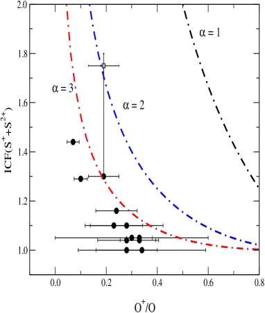
Figure 6: Ionisation correction factors, derived from our tailored photo-ionisation models for the objects in our sample. The continuous line represents the predictions by the scheme of Peimbert & Costero (1978). The dashed-dotted lines corresponds to the fits to Stasińska (1978) models of Barker (1980) for $\alpha$=3 and $\alpha$=2, as labelled. Finally, the dashed line represents the fit to Stasińska (1990) models by Izotov et al. (1994).

Another approach has been suggested by Mathis & Rosa (1991) who propose the use of both O⁺/O⁺⁺ and S⁺/S⁺⁺ to derive the ICFs for various elements exploiting the fact that models which provide given values of these two ratios have similar ICFs, even if they have different geometry, chemical composition or ionising source. They then derive the various ICFs as a polynomial fitting to these ratios.

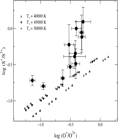
Figure 7: The S⁺/S²⁺ vs O⁺/O²⁺ diagram for the observed HII galaxies as compared with results from photo-ionisation models (see text for details).

When trying to use this method, the first question to ask is to what extent the model sequences reproduce the ionisation structure of the observed HII galaxies. We can check this by comparing the observationally derived ionic fractions and those computed by models. Figure 7 shows the S⁺/S²⁺ vs O⁺/O²⁺ values as derived from observations as compared to those predicted by our models for the objects of the sample. Models with Z/Z_⊙ 0.05 and 0.1 and 0.2 are shown. Open triangles, filled triangles and crosses correspond to stellar effective temperatures of 40,000, 45,000 and 50,000 K and the ionisation parameter varies between 10 ^-3 and 10^-2 in steps of 0.25 dex. As we can see, models distribute along a narrow diagonal band. This is to be expected since the quotient of these two ionic fractions is the “eta parameter” of Vílchez & Pagel(1988) and constitutes a measure of the “softness” of the ionising radiation. Therefore, nebula ionised by sources with similar spectral energy distribution should lie along a straight line in the diagram. The observed values are adequatelly reproduced by the models, given the large errors involved, for the objects of intermediate excitation. Significant deviations are however found for both high excitation objects, to the left of the diagram, and low excitation ones, to the right, in both cases in the sense of the models predicting lower values of S⁺/S²⁺ than observed. Figure 8 shows a comparison of the total sulphur abundances computed with the ICFs of Mathis & Rosa (1991) and those found in this work. In general, Mathis & Rosa’s provides S/H values systematically larger than ours by about 0.15 dex which is inside the quoted uncertainty. Two objects however deviate significantly: IIZw40 and UM461 which are the objects with the highest excitation in our sample.

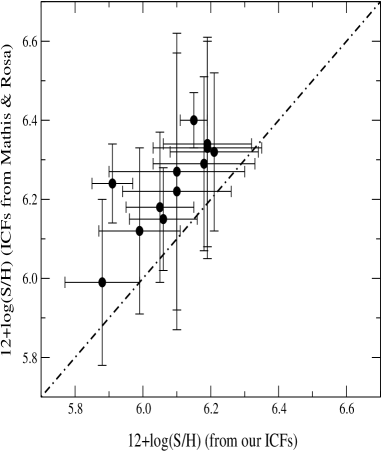
Figure 8: A comparison of the total sulphur abundances derived using Mathis & Rosa (1991) and our Ionisation correction factors. The dashed-dotted line represents the 1:1 relation.

4.3 Total abundances

The relation between the metallicity, represented by 12+log(O/H), and the N/O abundance ratio, assuming N/O = N⁺/O⁺ is plotted in Figure 9 for the observed sample of objets (solid circles) together with data corresponding to HII galaxies in the literature (open circles). Two locations for the sun are shown in the diagram, the one with the lowest N/O ratio corresponds to the data by Anders & Grevesse (1989). The other solar symbol corresponds to the more recent data of Allende Prieto et al. (2001) for oxygen and Holweger (2001) for nitrogen. Most observed objects cluster around a constant value of log(N/O) = -1.5. A couple of objects however show N/O ratios larger than expected for their low oxygen abundances. The most deviating datum corresponds to Mrk709 which shows an N/O ratio close to solar and an oxygen abundance of about one tenth solar. Our emission line data agree well with those of Terlevich et al. (1991) and the derived t_e([OIII]) and t_e([SIII]) are equal within the errors, which suggests that the oxygen abundance is probably well derived. This particular object, however, also shows relatively intense lines of [OI] $\lambda$ 6300 Å and [SII] $\lambda\lambda$ 6716, 6731 Å and has the lowest value of the equivalent width of H$\beta$ in our sample. Therefore it might constitute a case for a relatively evolved galaxy in which the contribution by shocks originated from stellar winds and/or supernovae is important. The large N/O abundance derived could be due to the enhancement of the [NII]$\lambda\lambda$ 6548, 6584 Å by the shock contribution.

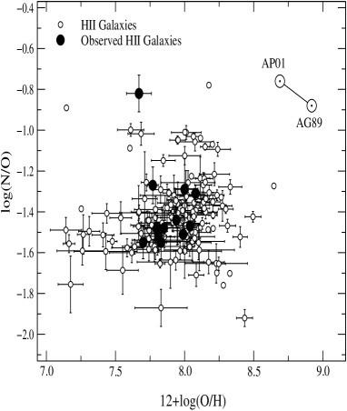
Figure 9: The N/O ratio as a function of total oxyen abundance for the objects in our sample and HII galaxy data in the literature.

The relation between the metallicity, represented by 12+log(O/H), and the S/O abundance ratio is plotted in Figure 10 for our sample objects and HII galaxies compiled from the literature. Solid circles represent the data of this work while solid squares circles correspond to data by Skillman & Kennicutt (1993) on IZw18 and Skillman et al. (1994) on UGC4483. In both cases the S²⁺ abundances have been derived from the near infrared [SIII] lines. We have added to the graph data by Izotov et al. (1994, 1997) and Izotov & Thuan (1998) represented by open circles, where the S²⁺ abundances have been derived from the weak [SIII]$\lambda$ 6312 Å line. In this latter case we have recomputed the abundances to take properly into account the observational errors and we have applied the sulphur ICFs calculated from Barker (1980) which fits best our observations.

Again two solar symbols are shown in the diagram, one corresponding to the data by Anders & Grevesse (1989) and a higher one in which the more recent value of the solar oxygen abundance by Allende Prieto et al. (2001) is adopted. In this case, all the observed objects show S/O ratios which are below the new S/O solar ratio, suggesting that some revision of the solar sulphur abundance might be needed. The sources of observational errors in the measurement of the auroral lines and the uncertainties due to the modelling of the unobserved properties of the nebulae lead to recognized difficulties in ascertaining any real trends of the relation between S/O and O/H. The data are inconclusive and keep some open questions about the behaviour of the S/O ratio in the regime of low metallicity. More good quality data are obviously needed reaching the near IR in order to explore this behaviour which can convey important information about the nucleosynthesis processes in high mass stars and the initial mass function at the high mass end. Data in the mid-IR to obtain [SIV] intensities would also help to clarify this question.

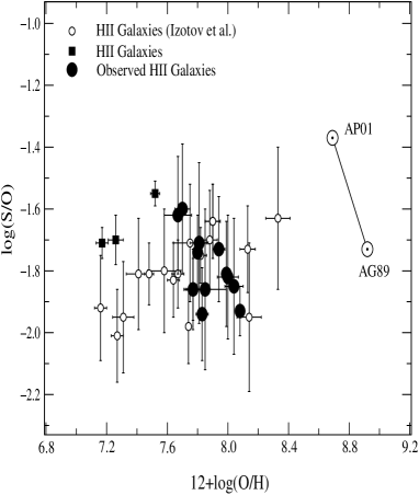
Figure 10: The S/O ratio as a function of total oxyen abundance for the objects in our sample and HII galaxy data in the literature.

Finally, we have added to the empirical calibration of the metallicity parameter, S₂₃= ([SII]+[SIII])/H$\beta$, (Díaz & Pérez-Montero, 2000) our observed HII galaxies and also recent data from Kennicutt & Garnett (2000) corresponding to HII regions in the Galaxy and the Magellanic Clouds; Oey et al. (2000) corresponding to HII regions in the LMC; and the sample of HII regions by Castellanos et al. (2002). This calibration, although showing a substantial scatter, has the potentiallity of remaining single-valued up to solar metallicity. This is specially important in the case of HII galaxies most of which show values of the commonly used oxygen abundance parameter R₂₃ in the turn-over region of the abundance calibration. In fact, this precludes the knowledge of the true abundance distribution of HII galaxies. However, more data points are needed in order to reduce the scatter of the relation and fill the existing gap at the low abundance end.

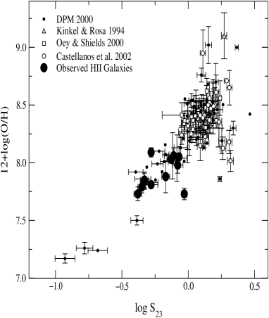
Figure 10: The parameter $S_{23}$ plotted against the metallicity of the regions

5 Conclusions

We have analyzed long-slit spectrophotometric observations of a sample of 12 HII galaxies in the red and far red including the auroral and nebular [SIII] lines at $\lambda$ 6312 Å and $\lambda\lambda$ 9069 and 9532 Å respectively and the [OII] lines at $\lambda\lambda$ 7319 and 7330 Å. For all the objects, previous data in the blue-visible exist and it has therefore been possible to derive directly at least three line temperatures: t([OII]), t([OIII]) and t([SIII]). For 7 of the 12 observed objects it has also been possible to measure t([SII]). The temperatures for [OII] and [SII] are found to be representative of the same zone. Regarding t([OII]) and t([OIII]), their values cluster around those predicted by simple photo-ionisation models with intermediate density (100 cm^-3). However, some objects show values of t([OII]) which are significantly below the theoretical relation. This could in principle be due to a higher value of the density that affects the derivation of t([OII]). The fact of using a t([OII]), representative of the low ionisation zone, computed from photo-ionisation model sequences instead of that directly derived, can lead to underestimate the O⁺/H⁺ ionic abundance and hence the total oxygen abundance by factors much larger than quoted observational errors. Regarding t([SIII]) most of the observed objects show values which are slightly larger than those predicted from t([OIII]) by the linear fit given by Garnett (1989) on the base of photo-ionisation models. The effect can be significant for the high excitation objects.

For all the objects in the sample we have derived the ionic fractions of O, N and S and have computed ICF for nitrogen and sulphur from detailed photo-ionisation model fits to the data. We have confirmed the validity of the commonly taken assumptions of O/H = (O⁺+O⁺⁺)/H⁺ and N/O = N⁺/O⁺. Regarding sulphur, our ICFs for (S⁺+S⁺⁺) are best reproduced by Barker (1980) approximation formula. On the other hand, the ionisation structure of the observed regions are not adequatelly reproduced by theoretical models for relatively low exctitation objects and the total sulphur abundances as computed with the ICF calculated from the method of Mathis & Rosa (1991) based on this ionisation structure are systematically larger than those found in this paper.

Finally, regarding total abundances, the N/O ratio for our observed objects, and also for a large sample of HII galaxies in the literature, shows values below solar, although it is far from being constant. In fact it spans almost an order of magnitude, with some objects having an N/O ratio too high for their derived oxygen abundance. For the S/O observational errors are still too high to ascertain the reality of any existing trend.

References

- [1] Allende Prieto, C., Lambert, D.L. & Asplund, M. 2001, ApJ, 556, 63
- [2] Anders, E. & Grevesse, N., 1989 Geochimica et Cosmochimica Acta, 53, 197.
- [3] Castellanos, M., Díaz, A.I. & Terlevich, E. 2002, MNRAS, 329, 315.
- [4] Cerviño, M. & Mas-Hesse, J.M. 1994, A&A, 284, 749
- [5] De Robertis, M.M., Dufour, R.J. & Hunt, R.W. 1987, JRASC, 81, 195.
- [6] Díaz, A.I., Terlevich, E., Ví lchez, J.M., Pagel, B.E.J. & Edmunds, M.G. 1991, MNRAS, 253, 245.
- [7] Díaz, A.I. 1994, in Violent star formation: from 30Doradus to Quasars. Ed. G. Tenorio-Tagle. Cambridge Univ. Press, Cambridge, p. 30.
- [8] Díaz, A.I. 1999, Ap&SS, 263, 143.
- [9] Díaz, A.I., Castellanos, M., Terlevich, E. & Garcí a-Vargas, M.L. 2000, MNRAS, 318, 462.
- [10] Díaz, A.I., Pagel, B.E.J. & Wilson, I.R.G. 1985, MNRAS, 212, 737.
- [11] Díaz, A.I., Pérez-Montero, E. 2000, MNRAS, 312, 130.
- [12] Ferland, G.J., HAZY: A brief introduction to CLOUDY. Univ. Kentucky internal report.
- [13] Galavis, M.E., Mendoza, C. & Zeippen, C.J. 1995, A&AS, 111, 347.
- [14] Garnett, D.R. 1989, ApJ, 345, 282.
- [15] Garnett, D.R. 1992, AJ, 103, 1330.
- [16] Garnett, D.R., Dufour, R.J., Peimbert, M., Torres-Peimbert, S., Shields, G.A., Skillman, E.D., Terlevich, E.& Terlevich, R. 1995, ApJ, 449, 77.
- [17] Grevesse, N.& Sauval, A.J.. 1998, SSRv. 85, 161.
- [18] Guseva, N, Izotov, Y.L. & Thuan, T.X. 2000, ApJ, 531, 776.
- [19] Holweger, H. 2001, in Joint SOHO/ACE Workshop: Solar and galactic composition. Ed. R.F. Wimmer-Schweimgruber, p. 23.
- [20] Hunter, D.A. & Hoffman, L. 1999, A&A, 117, 2789.
- [21] Izotov, Y.L., Thuan, T.X. & Lipovetsky, V.A. 1994, ApJ, 435, 647.
- [22] Izotov, Y.L., Thuan, T.X. & Lipovetsky, V.A. 1997, ApJS 108, 11.
- [23] Izotov, Y.L.& Thuan, T.X. 1998, ApJ, 500, 188.
- [24] Kennicutt, R.C. Jr., Bresolin, F., French, H. & Martin, P. 2000, ApJ, 537, 589.
- [25] Kunth, D. & Sargent, W.L.W. 1983, ApJ, 273, 81.
- [26] Lennon, D.J. & Burke, V.M. 1994, A&A, 287, 885.
- [27] McLaughlin, B.M.& Bell, K.L. 1998, JPhB, 31, 4317.
- [28] Masegosa, J., Moles, M. & Campos-Aguilar, A. 1994, ApJ 420, 576.
- [29] Melnick, J., Moles, M., Terlevich, R.& Garcí a-Pelayo, J.M. 1987, MNRAS, 226, 849.
- [30] Oey, M.S., Dopita, M.A., Shields, J.C. & Smith, R.C. (2000), ApJSS, 128, 511.
- [31] Pagel, B.E.J., Edmunds, M.G., Blackwell, D.E., Chun, M.S. & Smith, G., 1979, MNRAS, 189, 95.
- [32] Pagel, B.E.J., Simonson, E.A., Terlevich, R.J. & Edmunds, M.G. 1992, MNRAS, 255, 325.
- [33] Pagel, B.E.J. 1997 in Nucleosynthesis and chemical evolution of galaxies. Cambridge University Press.
- [34] Peimbert, M. 1967, ApJ, 150, 825.
- [35] Pilyugin, L.S. 2000, A&A, 362,325.
- [36] Ramsbottom, C.A., Bell, K.L. & Stafford, R.P. 1996, ADNDT, 63, 57.
- [37] Schaerer, D. & de Koter, A. 1997, A&A, 322, 598.
- [38] Schulte-Ladbeck, R.E., Crone, M.M. & Hopp, U. 1998, ApJ, 493, 23.
- [39] Shaw, R.A. & Dufour, R.J. 1995, PASP, 107, 896.
- [40] Skillman, E.D. & Kennicutt, R.C. 1993, ApJ 411, 655.
- [41] Skillman, E.D., Terlevich, R.J., Kennicutt, R.C., Garnett, D. & Terlevich, E. 1994, ApJ, 431, 172.
- [42] Stasińska, G. 1980, A&A, 84, 320.
- [43] Stasińska, G. 1990, A&AS, 83, 501.
- [44] Tayal, S.S. 1997, ApJS, 111, 459.
- [45] Tayal, S.S. & Gupta, G.P. 1999, ApJ, 526, 544.
- [46] Telles, E., Melnick, J. & Terlevich, R. 1997, MNRAS, 288, 78.