Statistical Interpretation of LMC Microlensing Candidates.

Abstract

: Galaxy: halo – dark matter

1 Introduction

The rotational curve of disc in the spiral galaxies shows the existence of dark matter in the halos of galaxies. MAssive Compact Halo Objects (MACHOs) like brown dwarfs, white dwarfs, neutron stars and black holes could be candidates for the baryonic component of the dark halo. The gravitational microlensing technique was proposed by Paczyński (1986) for indirect detection of MACHOs in the halo of our Galaxy. The effect of microlensing is a temporary light amplification of background stars due to MACHOs passing through our line of sight. Since early 1990s several groups like AGAPE, DUO, EROS, MACHO, OGLE and PLANET have contributed to this field and began monitoring millions of stars in the Large and Small Magellanic Clouds (LMC and SMC). In the direction of LMC, the MACHO collaboration observed $13-17$ candidates from $5.7$ years observation of $11.9$ million stars (Alcock et al. 2000). EROS also observed LMC-1 from EROS I photometric plates (Ansari et al. 1996) and the other four events from EROS II (Lasserre et al. 2000; Spiro & Lasserre 2001; Milsztajn & Lasserre 2001). Interpretation of the observed results within the framework of Galactic models has been a matter of debate in recent years. By comparing the expected and the observed numbers of microlensing events, it is possible to evaluate the mass fraction of the halo in the form of MACHOs and also the mean mass of MACHOs.
As an example, in the standard Galactic model, MACHO group obtained the optical depth of microlensing events $\tau_{LMC}=1.2^{+0.4}_{-0.3}\times 10^{-7}$ in the direction of LMC (Alcock et al. 2000) and this result is consistent with the theoretical expectation if $\sim 0.2$ times the halo mass in this model is made up of MACHOs. The mean value of the duration of events also indicates that the mean mass of lenses should be $\sim 0.5M_{\odot}$, which means that the masses of MACHOs are about the same as those of white dwarf stars. The EROS group also put a constraint on the fraction of halo in the form of MACHOs, with the masses of lenses in the range of $10^{-7}M_{\odot}$ to $4M_{\odot}$, excluding that no more than $40$ per cent of the standard halo is made of objects with up to one solar mass at $95$ per cent confidence (Spiro & Lasserre 2001).
It should be mentioned that the conclusions of EROS and MACHO groups on the contribution of MACHOs to the mass of the dark halo and the mean mass of lenses is in some cases at variance with other observations. The outline of this contradiction is as follows (Gates & Gyuk 2001).

• To allow the mass of the MACHOs to be in the range proposed by microlensing observations, the initial mass function of MACHO progenitors of the Galactic halo should be different from the disc (Adams & Laughlin 1996; Chabrier, Segretain & Mera 1996). Limits on the initial mass function of the halo arise from both low- and high-mass stars. Low mass stars $(M<1M_{\odot})$ should still be active and visible, and heavy stars $(M>8M_{\odot})$ have evolved into Type II supernovae and have ejected heavy elements into the interstellar medium.

• If there were as many white dwarfs in the halo as suggested by microlensing experiments they would increase the abundance of heavy metals via Type I Supernova explosions. Canal, Isern $\&$ Ruiz-Lapuente (1997) used this phenomenon and showed that halo fraction in the white dwarfs has to be less than $5--10$ per cent. To be compatible with the gravitational microlensing results, they proposed that the star-formation process in the halo is possibly different from the local observations for single as well as binary stars.

• Recently Green & Jedamzik (2002) mentioned that the observed distribution of microlensing duration is not compatible with what is expected from the standard halo model. They showed that the distribution of microlensing candidates in terms of the duration of events is significantly narrower compared to that expected from the standard halo model at $90-95$ per cent confidence.

Here we extend the earlier work of Green & Jedamzik (2002) (i) to include the EROS microlensing events (ii) to take into account the contribution of the LMC and luminous components of the Milky Way in the microlensing events, and (iii) and finally to consider the non-standard halo models (Alcock et al. 1996). The mass function of lenses was chosen to be a Dirac-delta function where the peak of the function and the fraction of halo in the form of MACHOs in each Galactic model are chosen according to the likelihood analysis of the MACHO group. We generate the expected distribution of events, using the observational efficiency of the experiments and compare them with the distributions of microlensing data. This comparison is performed by a Monte-Carlo simulation to generate the width and the mean of distribution and compare them with the observed data. The paper is organized as follows. In Section 2 we give a brief review of Galactic models and generate the expected distribution of events by considering the EROS and MACHO observational efficiency. Section 3 compares the expected distribution in the Galactic models and observed data using statistical parameters. The results are discussed in Section 4.

2 galactic models and the expected microlensing distribution

This section discusses the relevant components of the structure of the Milky Way, including: the power-law models of the Milky Way halo, luminous parts of Milky Way such as the disc and spheroid, and also the LMC itself. These elements can be combined to build various Galactic models that have been discussed by Alcock et al. (1996). Here we use the mass function of the MACHOs and their contribution to the mass of Galactic halo according to the likelihood analysis of the MACHO group. We obtain the theoretical distribution of the rate of events in the direction of the LMC in each model. The observational efficiencies of the EROS and MACHO experiments are applied to obtain the expected distribution of events as a function of the duration of events in these models.

2.1 Power-law halo models

Here we use the largest known set of axisymmetric models of Galactic halo, the so-called ”power-law Galactic” models (Evans 1994). The density of these models in the cylindrical coordinate system are given by

$$\rho(R,z)=\frac{{V_{a}}^{2}{R_{c}}^{\beta}}{4\pi Gq^{2}}\times\frac{{R_{c}}^{2}(1+2q^{2})+R^{2}(1-\beta q^{2})+z^{2}[2-(1+\beta)/q^{2}]}{({R_{c}}^{2}+R^{2}+z^{2}/q^{2})^{(\beta+4)/2}},$$ (1)

where $R^{2}=r^{2}+z^{2}$, $R_{c}$ is the core radius and $q$ is the flattening parameter which is the axial ratio of the concentric equipotentials. $q=1$ represents a spherical $(E0)$ halo and $q\sim 0.7$ gives an ellipticity of about $E6$. The parameter $\beta$ determines whether the rotational curve asymptotically rises, falls or is flat. At asymptotically large distances from the centre of the Galaxy in the equatorial plane, the rotation velocity is given by $V_{circ}\sim R^{-\beta}$. Therefore $\beta=0$ corresponds to a flat rotation curve, $\beta<0$ is a rising rotation curve and $\beta>0$ is a falling curve. The parameter $V_{a}$ determines the overall depth of the potential well and hence gives the typical velocities of objects in the halo. The velocity dispersion of halo also is given by

$$\sigma_{R}^{2} = \sigma_{z}^{2}=\frac{V_{a}^{4}R_{c}^{2\beta}}{8\pi Gq^{2}}\frac{2q^{2}R_{c}^{2}+(1-\beta)q^{2}R^{2}+[2-(1+\beta)q^{-2}]z^{2}}{(1+\beta)(R_{c}^{2}+R^{2}+z^{2}q^{-2})^{\beta+2}}$$ (2)

$$\sigma_{\phi}^{2} = \frac{V_{a}^{4}R_{c}^{2\beta}}{8\pi Gq^{2}}\frac{2q^{2}R_{c}^{2}+[2+2\beta-(1+3\beta)q^{2}]R^{2}+[2-(1+\beta)q^{-2}]z^{2}}{(1+\beta)(R_{c}^{2}+R^{2}+z^{2}q^{-2})^{\beta+2}}.$$ (3)

The parameters of power-law halo models are indicated in Table 1.

2.2 Luminous components of the Milky Way and LMC

The luminous and non-halo components of the Milky Way are the galactic disc and spheroid. Here we also use the contribution of the LMC disc and halo. We model the density of the thin and thick discs of the Milky Way and LMC as double exponentials (Binney & Tremaine 1987):

$$\rho(R,z)=\frac{\Sigma_{0}}{2h}\exp\left[-\frac{R-R_{0}}{R_{d}}\right]\exp\left[-\frac{|z|}{h}\right]$$ (4)

where $z$ and $R$ are cylindrical coordinates, $R_{0}$ is the distance of the Sun from the centre of the Galaxy, $R_{d}$ is the scalelength, $h$ is the scaleheight of the disc and $\Sigma_{0}$ indicates the column density of the disc. For the thin disk of the Milky Way, which mainly consists of the star population and gases, these parameters are: $R_{d}=4kpc$, $h=0.3kpc$, $\Sigma_{0}=50M_{\odot}pc^{-3}$, $R_{0}=8.5kpc$ and $\sigma_{v}=31km/s$, where $\sigma_{v}$ is the adopted one-dimensional velocity dispersion perpendicular to our line of sight. For the case of maximal disk, all the parameters are the same as the thin disk except $\Sigma_{0}=80M_{\odot}pc^{-3}$. For the thick disc of the Milky Way, the parameters are: $R_{d}=4kpc$, $h=1.0Kpc$, $\Sigma_{0}=40M_{\odot}pc^{-3}$, $R_{0}=8.5kpc$ and $\sigma_{v}=49km/s$. The mass function of the disc component is taken according to the observations with the Hubble Space Telescope (Gould, Bahcall & Flynn 1997). Here we are also interested in considering the rate of microlensing by the LMC, the so-called self-lensing. The LMC disc parameters taken from Gyuk et al. (2000) are $R_{d}=1.57kpc$, $h=0.3kpc$, $\sigma_{v}=25km/s$.
The other luminous component that may have a contribution to the microlensing events is the Milky Way spheroid. The spheroid density is given by (Guidice el al. 1994; Alcock et al. 1996):

$$\rho_{spher}=1.18\times 10^{-4}(r/R_{0})^{-3.5}M_{\odot}pc^{-3},$$ (5)

This density profile clearly must be cut off at small distances from the center of Galaxy, but this is irrelevant here since the LMC line of sight is always at $r>0.99R_{0}$. We take the dispersion velocity for this structure $\sigma_{v}=120km/s$.

2.3 Expected rate of events in the Galactic models

In this part we use the Galactic models to obtain the rate of the duration of events. To obtain the differential rate of duration of events we need entire phase space distribution function. The differential rate is give by

$$d\Gamma=\frac{1}{m}F({\bf v},{\bf x})cos\theta u_{T}R_{E}v_{t}d^{3}vdxd\alpha,$$ (6)

where $m$ is the mass of the lenses, $F(\bf{v},\bf{x})$ is the phase space distribution of the MACHOs, $u_{T}R_{E}$ is the radius of the microlensing ”tube” at position $x$ from the observer, $u_{T}R_{E}d\alpha$ is the cylindrical segment of that tube and $v_{t}$ is the transverse velocity of the MACHO in the frame of the microlensing tube (Griest 1991). We use numerical methods to obtain the differential rate of events in the standard halo model, power-law halo models and also in the disc, spheroid and LMC (Alcock et al. 1995). The Contributions of the components of the Milky Way and LMC to the total differential rate of events are given by:

$$\frac{d\Gamma}{dt}={\it f}\frac{d\Gamma}{dt}(MWhalo)+\frac{d\Gamma}{dt}(disk)+\frac{d\Gamma}{dt}(Spheroid)+\frac{d\Gamma}{dt}(LMC),$$ (7)

The first term is the halo contribution in which f is the halo fraction in the form of MACHOs. Second, third and fourth terms are the contributions of the disc, spheroid and LMC itself.

		Model :	$S$	$A$	$B$	$C$	$D$	$E$	$F$	$G$
	(1)	Description	Medium	Medium	Large	Small	E6	Maximal disk	thick disk	thick disk
	(2)	$\beta$	–	0	-0.2	0.2	0	0	0	0
	(3)	$q$	–	1	1	1	0.71	1	1	1
	(4)	$v_{a}(km/s)$	–	200	200	180	200	90	150	180
	(5)	$R_{c}(kpc)$	5	5	5	5	5	20	25	20
	(6)	$R_{0}(kpc)$	8.5	8.5	8.5	8.5	8.5	7	7.9	7.9
	(7)	$\Sigma_{0}(M_{\odot}/pc^{2})$	50	50	50	50	50	80	40	40
	(8)	$R_{d}(kpc)$	3.5	3.5	3.5	3.5	3.5	3.5	3	3
	(9)	$z_{d}(kpc)$	0.3	0.3	0.3	0.3	0.3	0.3	1	1

Table 1: The parameters of eight Galactic models. The first line indicates the description of the models; the second line, the slope of the rotation curve $(\beta=0$ flat, $\beta<0$ rising and $\beta>0$ falling); the third line, the halo flattening ($q=1$ represent spherical); the fourth line, $(v_{a})$, the normalization velocity; the fifth line, $R_{c}$, the halo core; the sixth line, the distance of the Sun from the centre of the Galaxy; the seventh line, the local column density of the disc ($\Sigma_{0}=50$ for canonical disc, $\Sigma_{0}=80$ for a maximal thin disc and $\Sigma_{0}=40$ for a thick disc); the eighth line, the disc scalelength; and the ninth line, the disk scalehight.

The parameter f and the mass function of MACHOs, which are taken to be a $\delta$-functions, can be obtained by the likelihood analysis method. Here we use the results of Alcock et al. (2000) for the $S,B$ and $F$ models and that of Alcock et al. (1997) for $A,C,D,E$ and $G$ models as shown in Table 2.

	Events	Model	Halo	$m_{ML}(M_{\odot})$	$f_{ML}$
	13	S	medium	0.54	0.20
	17	S	medium	0.72	0.22
	6	A	medium	0.32	0.41
	8	A	medium	0.32	0.55
	13	B	large	0.66	0.12
	17	B	large	0.87	0.14
	6	C	small	0.21	0.61
	8	C	small	0.21	0.83
	6	D	E6	0.31	0.37
	8	D	E6	0.31	0.50
	6	E	max disk	0.04	2.8
	8	E	max disk	0.04	$>1$
	13	F	big disk	0.19	0.39
	17	F	big disk	0.25	0.44
	6	G	big disk	0.21	0.71
	8	G	big disk	0.20	0.97

Table 2: The maximum likelihood estimates of MACHO mass m, halo fraction ${\it f}_{ML}$, for the eight Galactic models are shown in this table. The first column shows the number of detected microlensing events; the second column indicates the eight Galactic models, described in Table 1; the specifications of the models are given in the third column; and the fourth and fifth columns show the results of maximum likelihood analysis for the mass of MACHO and halo fraction in the form of MACHOs.

The results of numerical calculations for the rate of events are shown in Fig. 1.

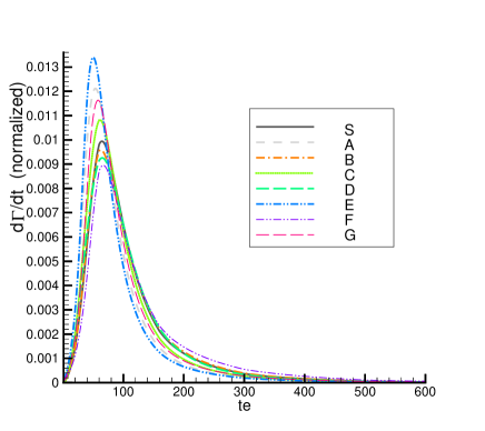
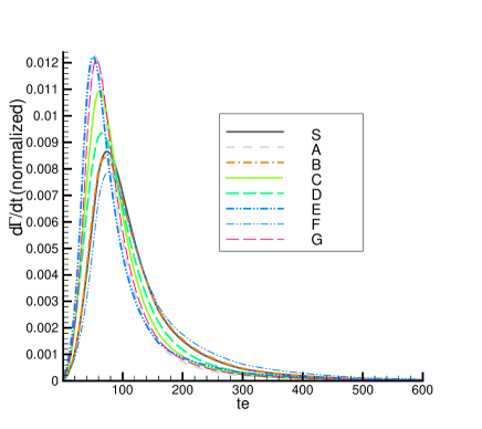
Figure 1: Theoretical differential rate of events as a function of the Einstein crossing time $t_{E}$ in the models described in Table 1. All the distributions are normalized to the total number of events in each model. According to likelihood analysis the mass function and halo fraction depend on the microlensing candidates that have been obtained by the criteria A or B. The left and right panels show the distributions of events that used the results of the A or B candidates, respectively (Alcock et al. 2000, 1997).

In order to deduce the expected distribution we need to have a reasonable knowledge of the detection efficiency of the experiments. The detection efficiency for individual events depends on many factors such as the impact parameter $u_{0}$, the moment of minimum impact parameter $t_{0}$, the duration of the event $t_{e}$, stellar magnitude of the lensed star, the strategy of observation and the weather conditions. Averaging over the parameters one can obtain the efficiency as a function of the duration of events $\epsilon(t_{e})$. The observational efficiencies of the EROS and MACHO experiments are given in (Alcock et al. 2000; Spiro & Lasserre 2001). Since in MACHO experiment two different and independent selection criteria have been used, we also use in our study two efficiencies called A and B according to the name of the criterion. The distribution of the rate of events expected from a Galactic model is obtained by multiplying the theoretical distribution by the observational efficiency:

$$\frac{d\Gamma}{dt}(expected)=\epsilon(t)\times\frac{d\Gamma}{dt}(model).$$ (8)

Fig.2 shows the expected distribution of the rate of events by applying the EROS, MACHO A and MACHO B efficiencies.

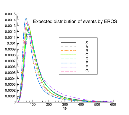
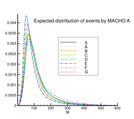
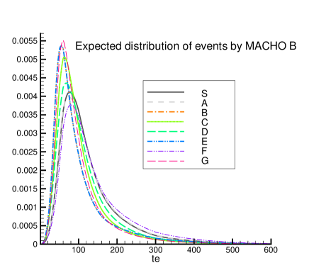
Figure 2: The expected normalized distributions of events shown in various Galactic models of $S,A,B,C,D,E,F$ and $G$. These distributions are obtained by multiplying the theoretical distributions of events to the observational efficiency.

3 Microlensing Candidates and Comparison with galactic models

In this section, the aim is to introduce the microlensing candidates observed by the EROS and MACHO groups and find the most likely models compatible with the data. Tables 3 and 4 show the microlensing candidates of the EROS and MACHO groups in terms of the duration of events in the direction of the LMC . The number of candidates depends on which of the criteria A or B have been applied in the algorithm of the data reduction process. Event 22 from the MACHO candidates seems likely to be a supernova of exceptionally long duration or an active galactic nucleus in a galaxy at redshift $z=0.23$, so it is ruled out as a microlensing candidate (Alcock et. al. 2001).

Event :	LMC-1	LMC-3	LMC-5	LMC-6	LMC-7
$t_{E}$ (days)	46	88	48	70	60

Table 3: EROS microlensing candidates in terms of the duration of events.

$Event:$	1	4	5	6	7	8	9	13	14	15	18	20	21	23	25	27
$t_{E}$ (days) B	44.	59	98	118	133	86	143	130	130	47	96	94	121	110	110	65
$t_{E}$ (days) A	41	55	92	112	125	81	–	122	122	45	90	–	113	104	104	–

Table 4: Microlensing candidates that have been observed by the MACHO during 5.7 years of observing 11.9 million LMC stars (Alcock et al. 2000). Sixteen microlensing candidate results are listed from the reduction process by criterion B and 13 events by criterion A. Events that have been selected by criterion A are included in B.

Figure 3: The expected distribution of the mean and the width of the distribution of the duration of events in the EROS, MACHO A and MACHO B experiments are shown for the standard model, and models A, B and C. The cross indicates the position of the observed value by these experiments. It is seen that non of the models gives the same width for the distribution of the duration or of the observed value.

Figure 4: The same distribution as Fig. 3 for models D, E, F and G. In these Galactic models also the observed value for the width of the duration is narrower than the expected value.

To compare the distribution of data in terms of the duration of events with the expected distribution in the Galactic models, we use the two statistical parameters called the the mean and the width of the distribution of events (Green and Jedamzik 2002). The width of the duration of events for the $N_{obs}$-th observed candidate is defined by

$$\Delta t_{E}=Max_{[j=1,N_{obs}]}(t_{j})-Min_{[j=1,N_{obs}]}(t_{j}).$$

We note that, considering the contribution of non-halo lenses, these statistical parameters depend on the best-fitting MACHO halo fraction and the mass function of the halo MACHOs. In the case of EROS candidates, the mean and the width of events according to Table 4 are obtained as $62$ and $42$ d, respectively. These parameters for the MACHO candidates, from Table 5, are $92$ and $84$ d for criterion A, and $99$ and $99$ d for criterion B. We perform a Monte Calro simulation which generates the distributions of the width and the mean of the duration of events from the expected theoretical distribution in the large sets of events where each set contains the same number of events from the observations. In other words, the number of events in each set is chosen to be equal to the number of candidates from an experiment. We chose five events in each set for generating EROS microlensing events and $13-16$ events for the MACHO events. Fig. 3 shows the two-dimensional distributions in terms of the width and the mean of the duration of events in the standard model and in models A, B and C. The crosses indicate the observed value of the mean and the width of the distribution of duration of microlensing candidates in the experiments. Fig. 4 shows the same distributions for models D, E, F and G. Since the typical mass function and the halo fraction in each model are taken from the likelihood analysis of the MACHO collaboration, the mean of the duration of candidates is compatible with what is expected from the models, while in all the diagrams it seems that the width of the observed value is much narrower than the expected distribution. To quantify this comparison, we obtain the fraction of generated event samples that yield a width smaller than the observation. Since in generating the microlensing events we take into account background events, we compare all the observed events and do not reject any of them as background. The result of this procedure, the fraction of simulations which have smaller width compared to observation in different Galactic models, are shown in Table 5. This fraction is less than about $5$ per cent in all models which means that the observed data, at least at the $95$ per cent level of confidence, are not compatible with the models.

	S	A	B	C	D	E	F	G
EROS Exp.	2	4	5	4	3	6	2	4
MACHO A Exp.	1	3	4	1.5	1	4	0.5	2.5
MACHO B Exp.	0.5	0.5	2	2.5	1	2	0.01	3

Table 5: The probability (per cent) that the the width the distribution of the duration of the observed candidates is smaller than that expected by the Galactic models. The first row indicates the name of the Galactic model and the first column shows the name of experiment. This probability is obtained by projecting the two-dimensional contour in Fig. 3 and 4 on the width axis and comparing the resulting distribution with the observed value. It is seen that the widths of the observed events are much smaller than the expected values from the models.

4 Conclusion

In this paper we have shown that in eight different Galactic models for the Milky Way, there is discrepancy between the expected distribution of microlensing events in terms of the duration of events and the data from the microlensing experiments. According to the likelihood analysis of the MACHO collaboration, two parameters have been obtained from the comparison of the models with the microlensing data: (i) the typical MACHO mass and (ii) the fraction of the halo mass in the form of MACHOs. To obtain the distribution of the duration of events, we used their results to generate the distribution of microlensing events in these halo models and added also the contribution of the non-halo components such as the disc, spheroid and LMC. After applying the observational efficiency the expected distributions of events were obtained.
We performed a Monte Carlo simulation to find the expected width of the distribution of the duration and showed that the observed width of the duration of candidates is smaller than that expected from the standard model (Green and Jedamzik 2002). We have shown that the same results are also valid for the non-standard models of the Milky Way. The contribution of the ”known” non-halo lenses in our calculation showed that this discrepancy may not be due to background events. One way to explain such a narrow distribution is that it could be due to the clumpy structure of MACHOs with small intrinsic velocity dispersion along the line of sight. If this were the case, the expected distribution of duration should be narrow compared to the ordinary halo case. The other advantage of this model could be decreasing that the mean mass of the MACHOs decrease compared to $\sim 0.5M_{\odot}$ .
The blending effect also changes our estimation of the actual value for the duration of events. The next generation of microlensing experiments, such as SUPERMACHO (Stubbs 1999) surveys with better sampling of microlensing light curves and high photometric precision, on the one hand, and increasing in the number of candidates, on the other, should reduce the ambiguity due to Poisson statistics. One of the proposed projects is to use two telescope working together, the first one to detect the microlensing events, and a follow-up 2-meter class telescope to observe the events precisely (Rahvar el al 2003). This type of survey could also partially break the degeneracy between the lens parameters by parallax, finite-size and double lens effects to localize the position and identify the mass of the lenses.

References

- [1996] Adams, F., Laughlin, G., 1996, APJ, 468, 586.
- [Alcock 1995] Alcock, C. et al. (MACHO), 1995, APJ 449, 28.
- [Alcock 1996] Alcock, C. et al. (MACHO), 1996, APJ 461, 84.
- [Alcock 1997] Alcock, C. et al. (MACHO), 1997, APJ 486, 697.
- [2000] Alcock C. et al. (MACHO), 2000, APJ 542, 281.
- [2001] Alcock, C. et al. (MACHO), 2001, APJ 550, L169.
- [1996] Ansari, R. et al. (EROS), 1996, A&A 314, 94.
- [1987] Binney S., Tremaine S., Galactic Dynamics, Princeton University Press (1987).
- [1996] Chabrier, G., Segretain, L., Mera D., 1996, APJ, 468, L21.
- [1997] Canal, R., Isern, J., Ruiz-Lapuente, P., 1997, APJ, 488, L35.
- [1994] Evans N. W., 1994, MNRAS 267, 333.
- [2001] Gates I. E., Gyuk, G., 2001, APJ 547, 786.
- [1] Gould A., Bahcall J. N., Flynn C., 1997, APJ 482, 913.
- [Green and Jedamzik 2002] Green A. M., Jedamzik K., 2002, A&A 395, 31.
- [Griest 1991] Griest, K. 1991, APJ, 366, 412.
- [Guidice et al. 1994] Guidice. G. F., Mollerach S & Roulet, E., 1994, Phys. Rev D 50, 2406.
- [Gyuk et al] Gyuk, G., Dalal, N., Griest K., 2000, APJ 535, 90.
- [Lasserre et al. 2000] Lasserre, T. et al. (EROS), 2000, A&A 355, L39.
- [2] Milsztain, A. and Lasserre, T. (EROS), 2001, Nucl. Phys. B (Proc. Suppl) 91, 413.
- [1986] Paczyński B., 1986, APJ 304, 1.
- [Rahvar et al. 2002] Rahvar S., Moniez M., Ansari R., Perdereau O. 2003, A&A, in press, preprint (astro-ph/0210563).
- [2001] Spiro M., Lasserre T, Cosmology and Particle Physics, edited by Durrer, R., Garcia-Bellido, J and Shaposhnikov, M (American Intitute of Physics),(2001) 146.
- [1998] Stubbs, C. W. 1999, APS, in the First meeting of the Northwest Section, The university of British Columbia Vancouver, BC, Canada, abstract #B2.02