Structure of pair winds from compact objects with application to emission from hot bare strange stars

Abstract

We consider a stationary, spherically outflowing wind consisting of electron-positron pairs and photons. We do not assume thermal equilibrium, and include the two-body processes that occur in such a wind: Møller and Bhaba scattering of pairs, Compton scattering, two-photon pair annihilation, and two-photon pair production, together with their radiative three-body variants: bremsstrahlung, double Compton scattering, and three-photon pair annihilation, with their inverse processes. In the concrete example described here, the wind injection source is a hot, bare, strange star. Such stars are thought to be powerful sources of pairs created by the Coulomb barrier at the quark surface. We present a new, finite-difference scheme for solving the relativistic kinetic Boltzmann equations for pairs and photons. Using this method we study the kinetics of the wind particles and the emerging emission for total luminosities of $L=10^{34}-10^{42}$ ergs s^-1 (the upper limit being set, at the moment, by computational limitations). We find the rates of particle number and energy outflows, outflow velocities, number densities, energy spectra, and other parameters for both photons and pairs as functions of the distance. We find that for $L>2\times 10^{35}$ ergs s^-1, photons dominate the emerging emission. For all values of $L$ the number rate of emerging pairs is bounded: $\dot{N}_{e}\lesssim\dot{N}_{e}^{\rm max}\simeq 10^{43}$ s^-1. As $L$ increases from $\sim 10^{34}$ to $10^{42}$ ergs s^-1, the mean energy of emergent photons decreases from $\sim 400-500$ keV to 40 keV, as the spectrum changes in shape from that of a wide annihilation line to nearly a blackbody spectrum with a high energy ($>100$ keV) tail. These results are pertinent to the deduction of the outside appearance of hot bare strange stars, which might help discern them from neutron stars.

1 Introduction

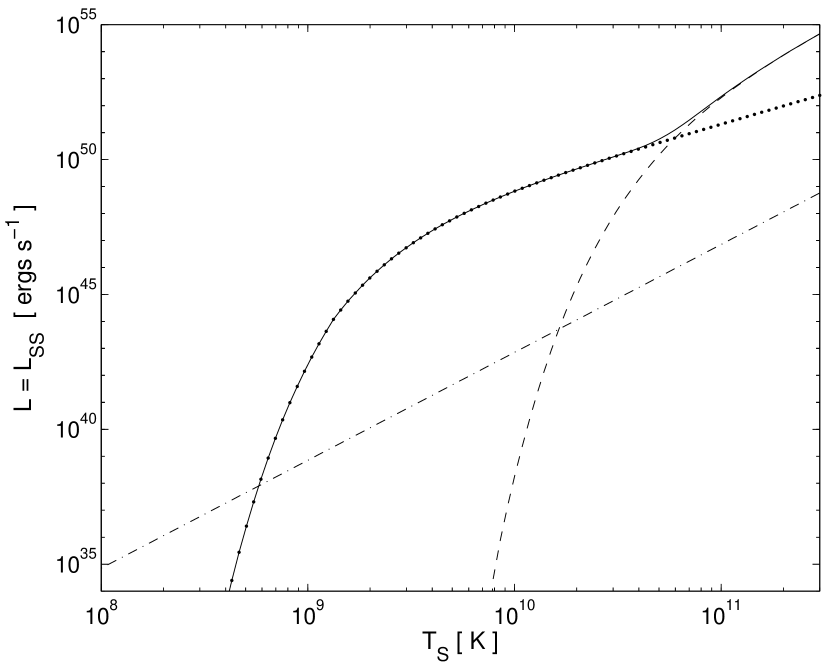
Figure 1: The luminosities of a hot, bare, strange star in $e^{+}e^{-}$ pairs (dotted line), in thermal equilibrium photons (dashed line), and the total (solid line) as functions of the surface temperature $T_{{}_{\rm S}}$. The upper limit on the luminosity in non-equilibrium photons, $L_{\rm neq}\lesssim 10^{-6}L_{\rm BB}$, is shown by the dot-dashed line, $L_{\rm BB}$ being the blackbody luminosity.

There is now compelling evidence that electron-positron ($e^{\pm}$) pairs form and flow away from many compact astronomical objects identified as neutron stars and black holes. Among these objects are pulsars (Sturrock 1971; Ruderman & Sutherland 1975, Arons 1981; Usov & Melrose 1996; Baring & Harding 2001), accretion-disc coronas of the Galactic X-ray binaries (White & Lightman 1989; Sunyaev et al. 1992), active galactic nuclei (Jelley 1966; Herterich 1974; Begelman, Blandford, & Rees 1984; Lightman & Zdziarski 1987; Sikora 1994; Blandford & Levinson 1995; Reynolds et al. 1996; Yamasaki, Takahara, & Kusunose 1999), cosmological $\gamma$-ray bursters (Eichler et al. 1989; Paczyński 1990; Usov 1992), etc. Several pair-production mechanisms are thought to operate in these objects. In pulsar magnetospheres, it is supposedly effected via conversion of single $\gamma$-photons into $e^{\pm}$ pairs in a strong magnetic field ($\gamma B\rightarrow e^{+}e^{-}B$), while in galactic nuclei, the pairs are created mostly in photon-photon collisions ($\gamma\gamma\rightarrow e^{+}e^{-}$). Thermal neutrinos and antineutrinos radiated by a very hot compact object may be absorbed near its surface and produce $e^{\pm}$ pairs ($\nu\tilde{\nu}\rightarrow e^{+}e^{-}$). For example in very young (age $<10$ s), compact objects with mean internal temperatures of $\sim 10^{11}$ K, the pair luminosity produced via this mechanism may be as high as $\sim 10^{51}$ ergs s^-1 (e.g., Eichler et al. 1989; Haensel, Paczyński, & Amsterdamski 1991), which is a typical luminosity of cosmological $\gamma$-ray bursters. Such pair winds are, therefore, discussed as possible sources of cosmological $\gamma$-ray bursts (for a review, see Piran 2000). Recently it was shown that strange stars, which are made entirely of deconfined quarks (e.g., Witten 1984; Alcock, Farhi, & Olinto 1986a; Haensel, Zdunik, & Schaeffer 1986), may also be powerful sources of $e^{\pm}$ pairs (Usov 1998, 2001a). In this case, the pairs are created in an extremely strong electric field at the quark surface. The thermal luminosity of a bare strange star in $e^{\pm}$ pairs depends on the surface temperature $T_{\rm S}$ and may be as high as $\sim 10^{50}-10^{51}$ ergs s^-1 at the moment of formation when $T_{\rm S}$ may be up to $\sim 10^{11}$ K (see Fig. 1). The luminosity of a young bare strange star in pairs may remain high enough ($\gtrsim 10^{36}$ ergs s^-1) for $\sim 10^{3}$ yr (Page & Usov 2002).

The properties of pair plasmas have been studied extensively, but most of the initial attention focused on plasmas in thermal equilibrium (e.g., Bisnovatyi-Kogan, Zeldovich, & Sunyaev 1971; Lightman 1981; Svensson 1982; Guilbert & Stepney 1985; Zdziarski 1985 and references therein). It is conceivable that such equilibrated plasmas exist in some objects. Very powerful pair winds are among these objects. For an energy injection rate of $\dot{\rm E}\gtrsim 10^{50}$ ergs s^-1, the pair density near a compact object of radius $\sim 10^{6}$ cm is very high, and the outflowing pairs and photons are nearly in thermal equilibrium almost up to the wind photosphere (e.g., Paczyński 1990). The outflow process of such a wind may be described fairly well by relativistic hydrodynamics (Paczyński 1986, 1990; Goodman 1986; Grimsrud & Wasserman 1998; Iwamoto & Takahara 2002). The emerging emission consists mostly of photons, so $L_{\gamma}\simeq\dot{\rm E}$. The photon spectrum is roughly a blackbody with a temperature of $\sim 10^{10}(\dot{\rm E}/10^{50}~{}{\rm ergs~{}s}^{-1})^{1/4}$ K. The emerging luminosity in $e^{\pm}$ pairs is very small, $L_{e}=\dot{\rm E}-L_{\gamma}\sim 10^{-6}L_{\gamma}\ll L_{\gamma}$. All this applies roughly down to $\dot{\rm E}\sim 10^{42}-10^{43}$ ergs s^-1. For $\dot{\rm E}<10^{42}$ ergs s^-1, which is the region we explore, the thermalization time for the $e^{\pm}$ pairs and photons is longer than the escape time, and pairs and photons are not in thermal equilibrium (see below). Recently, a brief account of the emerging emission from such a pair wind has been given by Aksenov, Milgrom, & Usov (2003). In the present paper, we study numerically the kinetics of $e^{\pm}$ pairs and photons in a stationary pair wind with energy injection rates $\dot{\rm E}\leq 10^{42}$ ergs s^-1, and find the structure of the wind and its emerging emission in $e^{\pm}$ pairs and photons. We assume that the outflowing wind consist of $e^{\pm}$ pairs and photons only. For the sake of concreteness, we take, in the present study, the input pair injection at the inner surface to correspond to a hot bare strange star. We use the Boltzmann equations for both $e^{\pm}$ pairs and photons (kinetic theory approach). The principal advantage of this approach compared to the Monte Carlo method is that it gives better photon statistics. Besides, the kinetic theory approach may still be used when the optical thickness is $\gg 1$, where the Monte Carlo method is ineffective. Some examples of the kinetic theory approach for investigations of non-equilibrium pair plasmas can be found in Fabian et al. (1986), Ghisellini (1987), Svensson (1987), and Coppi (1992). The remainder of the paper is organized as follows. In § 2 we formulate the equations that describe the pair wind from a hot bare strange star, and the boundary conditions. In § 3 we describe the computational method used to solve these equations. In § 4 we present the results of our numerical simulations. Finally, in § 5, we discuss some astrophysical applications.

2 Formulation of the problem

We consider, then, an $e^{\pm}$ pair wind that flows away from a hot, bare, unmagnetized, strange star with a radius of $R=10^{6}$ cm. We assume that the temperature is the same over the surface of the star. The pair flux $F_{e}$ from the unit surface of strange quark matter (SQM) depends on the surface temperature $T_{\rm S}$ only (Usov 1998, 2001a); and the pair wind is spherical. At a distance $r$ from the stellar center and at time $t$, the state of the plasma may be described by the distribution functions $f_{e^{\pm}}({\bf p},r,t)$ and $f_{\gamma}({\bf p},r,t)$ for positrons $(+)$, electrons $(-)$, and photons, respectively, where ${\bf p}$ is the momentum of particles. There is no emission of nuclei from the stellar surface, and therefore, the distribution functions of positrons and electrons are identical, $f_{e^{+}}=f_{e^{-}}=f_{e}/2$.

In the first run of our simulations the outflow of $e^{\pm}$ pairs from the stellar surface starts at the moment $t=0$, and its rate is constant with time ($\dot{\rm E}=10^{34}$ ergs s^-1) till the moment when a steady state is established in the examined space domain (see below). Then, the rate of the pair outflow increases instantly by a factor of 10, and the second run starts and continues till a new steady state is established, and so on. So, we find the structure of stationary $e^{\pm}$ pair winds and their emerging radiation for $\dot{\rm E}=10^{34},\,10^{35},\,...\,,\,10^{42}$ ergs s^-1.

2.1 Equations

We use the relativistic Boltzmann equations for the $e^{\pm}$ pairs and photons, whereby the distribution function for the particles of type $i$, $f_{i}(|{\bf p}|,\mu,r,t)$, ($i=e$ for $e^{\pm}$ pairs and $i=\gamma$ for photons), satisfies (e.g., de Groot, van Leeuwen, & van Weert 1980; Mihalas 1984; Mezzacappa & Bruenn 1993)

$$\frac{1}{c}\frac{\partial f_{i}}{\partial t}+\beta_{i}\left(\mu\frac{\partial f_{i}}{\partial r}+\frac{1-\mu^{2}}{r}\frac{\partial f_{i}}{\partial\mu}\right)=\sum_{q}\left[\tilde{\eta}_{i}^{q}-\chi_{i}^{q}f_{i}\right],$$ (1)

where $\mu=\cos\theta$, $\theta$ is the angle between the radius-vector ${\bf r}$ from the stellar center and the particle momentum ${\bf p}$, $p=|{\bf p}|$, and

$$\beta_{e}=v_{e}/c=[1-(m_{e}c^{2}/\epsilon_{e})^{2}]^{1/2},\,\,\,\,\,\,\,\beta_{\gamma}=1\,,$$ (2)

while

$$\epsilon_{e}=c[p^{2}+(m_{e}c)^{2}]^{1/2}\,\,\,\,\,\,\,{\rm and}\,\,\,\,\,\,\,\epsilon_{\gamma}=pc$$ (3)

are the energy of electrons and photons, respectively. Also $\tilde{\eta}_{i}^{q}$ is the emission coefficient for the production of a particle of type $i$ via the physical process labeled by $q$, and $\chi_{i}^{q}$ is the corresponding absorption coefficient. The summation runs over all considered physical processes that involve a particle of type $i$. Gravity is neglected (but its effects are briefly discussed in §5). This is a good approximation for $\dot{\rm E}>\tilde{L}_{\rm Edd}$, while for $\dot{\rm E}\lesssim\tilde{L}_{\rm Edd}$ the gravity effects may be important, where

$$\tilde{L}_{\rm Edd}\simeq 7\times 10^{34}(M/M_{\odot})~{}{\rm ergs~{}s}^{-1}\,,$$ (4)

is the Eddington luminosity for the pair plasma, above which radiation-pressure forces dominate over gravity.

The particle densities are given by

$$n_{i}(r,t)=\int f_{i}({\bf p},r,t)d{\bf p}\,.$$ (5)

For convenience of numerical simulations we use, instead of $f_{i}$, the quantities

$$E_{i}(\epsilon_{i},\mu,r,t)={2\pi\epsilon_{i}^{3}\beta_{i}f_{i}\over c^{3}},$$ (6)

as are used in the “conservative” numerical method, which can provide exact conservation of energy on a finite computational grid (see below). Since

$$\epsilon_{i}f_{i}d\mathbf{r}d\mathbf{p}={2\pi\epsilon_{i}^{3}\beta_{i}f_{i}\over c^{3}}d\mathbf{r}d\epsilon_{i}d\mu=E_{i}d\mathbf{r}d\epsilon_{i}d\mu\,,$$ (7)

we see that $E_{i}$ is the energy density in the $\{{\bf r},\mu,\epsilon_{i},\}$ phase space, in which the volume element is $d\mathbf{r}d\epsilon_{i}d\mu=4\pi r^{2}drd\epsilon_{i}d\mu$.

From equations (1) and (6) the Boltzmann equations can be written in terms of $E_{i}$ as

$$\frac{1}{c}\frac{\partial E_{i}}{\partial t}+{\mu\over r^{2}}\frac{\partial}{\partial r}(r^{2}\beta_{i}E_{i})+\frac{1}{r}\frac{\partial}{\partial\mu}\left[(1-\mu^{2})\beta_{i}E_{i}\right]$$

$$=\sum_{q}\left[\eta_{i}^{q}-\chi_{i}^{q}E_{i}\right],$$ (8)

where

$$\eta_{i}^{q}={2\pi\epsilon_{i}^{3}\beta_{i}\tilde{\eta}_{i}^{q}\over c^{3}}$$ (9)

This form of the Boltzmann equations is said to be “conservative”, in the case without gravity, because the “transport” terms can be written as a derivative of a flux divided by a volume (Harleston & Holcomb 1991). This allows one to develop a conservative finite difference code for numerical simulations and to carry out calculations with large time steps even for very large optical depths. In our simulations we use the Boltzmann equations (8) for both pairs and photons.

2.2 Boundary conditions

The computational boundaries are

$$r_{\rm int}<r<r_{\rm ext},\,\,\,\,\,\,\,0<t<t_{\rm st}\,,$$ (10)

where $r_{\rm ext}=1.65\times 10^{8}$ cm is chosen as the radius of the external boundary, and $t_{\rm st}$ is the time when the wind approaches stationary closely enough. The internal radius is that typical of a strange star ($r_{\rm int}=R$). At this radius, the injection rate of pairs is taken as (Usov 1998, 2001a)

$$\dot{N}_{e}^{\rm in}=4\pi R^{2}F_{e}\,,$$ (11)

where

$$F_{e}=3\times 10^{42}\exp\,(-0.593\zeta)$$

$$\times\left[\frac{\displaystyle\ln(1+2\zeta^{-1})}{\displaystyle(1+0.074\zeta)^{3}}+\frac{\displaystyle\pi^{5}\zeta}{\displaystyle 2(13.9+\zeta)^{4}}\right]\,{\rm cm}^{-2}{\rm s}^{-1},$$ (12)

and $\zeta=20(T_{\rm S}/10^{9}\,{\rm K})^{-1}$. The energy spectrum of injected pairs is thermal with temperature $T_{\rm S}$, and their angular distribution is isotropic for $0\leq\mu\leq 1$.

The energy injection rate is equal to the thermal luminosity of the strange star in $e^{\pm}$ pairs,

$$\dot{\rm E}=L_{\rm SS}=\dot{N}_{e}^{\rm in}[m_{e}c^{2}+(3/2)k_{\rm B}T_{\rm S}]\,,$$ (13)

where $k_{\rm B}$ is the Boltzmann constant (Usov 2001a). For the range of the energy injection rates we consider, $\dot{\rm E}=10^{34}-10^{42}$ ergs s^-1, the surface temperature is in a rather narrow range, $T_{\rm S}\simeq 4\times 10^{8}-10^{9}$ K (see Fig. 1).

The thermal emission of photons from the surface of a bare strange star is strongly suppressed if the surface temperature is not very high, $T_{\rm S}\ll 10^{11}$ K (Alcock et al. 1986a). The reason is that the plasma frequency of quarks in SQM is very large, $\hbar\omega_{\rm p}\simeq 20-25$ MeV, and only hard photons with energies $\epsilon_{\gamma}>\hbar\omega_{\rm p}$ can propagate in SQM. The luminosity in such hard photons, which are in thermodynamic equilibrium with quarks, decreases very fast for $T_{\rm S}\ll\hbar\omega_{\rm p}/k_{\rm B}$ (Chmaj, Haensel, & Slomiński 1991; Usov 2001a), and in our case when $T_{\rm S}$ is $\lesssim 10^{9}$ K, it is negligible (see Fig. 1). However, low-energy ($\epsilon_{\gamma}<\hbar\omega_{\rm p}$) photons may leave SQM if they are produced by a nonequilibrium process in the surface layer of thickness of $\sim c/\omega_{\rm p}\sim 10^{-12}$ cm (Chmaj et al. 1991). Recently, the emissivity of SQM in nonequilibrium quark-quark bremsstrahlung radiation has been estimated by Cheng & Harko (2003), taking into account the Landau-Pomeranchuk-Migdal effect, and it is shown that the SQM emission in nonequilibrium photons is suppressed at least by a factor of $10^{6}$ in comparison with blackbody emission (see Fig. 1). It was argued that SQM is a color superconductor with a very high critical temperature $T_{c}\sim 10^{11}-10^{12}$ K (Alford, Rajagopal, & Wilczek 1999; Alford, Bowers, & Rajagopal 2001). In this case, the nonequilibrium emission is suppressed further. In our simulations, we neglect the surface emission of photons altogether.

The stellar surface is assumed to be a perfect mirror for both $e^{\pm}$ pairs and photons. At the external boundary ($r=r_{\rm ext}$), the pairs and photons escape freely from the studied region, i.e., the inward ($\mu<0$) flux of both $e^{\pm}$ pairs and photons vanishes.

2.3 Physical processes in the pair plasma

Although the pair plasma ejected from the strange-star surface contains no radiation, as the plasma moves outwards photons are produced by pair annihilation ($e^{+}e^{-}\rightarrow\gamma\gamma$). Other two-body processes that occur in the outflowing plasma are Møller ($e^{+}e^{+}\rightarrow e^{+}e^{+}$ and $e^{-}e^{-}\rightarrow e^{-}e^{-}$) and Bhaba ($e^{+}e^{-}\rightarrow e^{+}e^{-}$) scattering, Compton scattering ($\gamma e\rightarrow\gamma e$), and photon-photon pair production ($\gamma\gamma\rightarrow e^{+}e^{-}$). Two-body processes do not change the total number of particles in a system, and thus cannot, in themselves, lead to thermal equilibrium. For this reason, we include radiative processes (bremsstrahlung, double Compton scattering, and three photon annihilation with their inverse processes) that change the particle number even though their cross-sections are at least $\sim\alpha^{-1}\sim 10^{2}$ times smaller than those of the two-body processes ($\alpha=e^{2}/\hbar c=1/137$ is the fine structure constant). Radiative pair production, $\gamma\gamma\leftrightarrow e^{+}e^{-}\gamma$, which is a radiative variant of photon-photon pair production, $\gamma\gamma\rightarrow e^{+}e^{-}$, is not essential and is ignored in our simulations. The processes we include are listed in Table 1.

3 The computational method

In the numerical scheme we define a grid in the $\{{\bf r},\mu,\epsilon\}$ phase-space as follows. The $r$ domain ($R<r<r_{\rm ext}$) is divided into $j_{\rm max}$ spherical shells whose boundaries are designated with half integer indices. The $j$ shell ($1\leq j\leq j_{\rm max}$) is between $r_{j-1/2}$ and $r_{j+1/2}$, with $\Delta r_{j}=r_{j+1/2}-r_{j-1/2}$ ($r_{1/2}=R$ and $r_{j_{\rm max}+1/2}=r_{\rm ext}$).

The $\mu$-grid is made of $k_{\rm max}$ intervals $\Delta\mu_{k}=\mu_{k+1/2}-\mu_{k-1/2}$: $1\leq k\leq k_{\rm max}$.

The energy grids for photons and electrons are different. They are both made of $\omega_{\rm max}$ energy intervals $\Delta\epsilon_{i,\omega}=\epsilon_{i,\omega+1/2}-\epsilon_{i,\omega-1/2}$: $1\leq\omega\leq\omega_{\rm max}$, but the lowest energy for photons is 0, while that for pairs is $m_{e}c^{2}$.

The quantities we compute are the energy densities averaged over phase-space cells

$$E_{i,\omega,k,j}(t)=\frac{1}{\Delta X}\int_{\Delta\epsilon_{\omega},\Delta\mu_{k},\Delta r_{j}}E_{i}d\epsilon d\mu r^{2}dr.$$ (14)

where $\Delta X=\Delta\epsilon_{\omega}\Delta\mu_{k}\Delta(r^{3}_{j})/3$ and $\Delta(r^{3}_{j})=r^{3}_{j+1/2}-r^{3}_{j-1/2}$.

Replacing the space and angle derivatives in the Boltzmann equations (6) by finite differences, we have the following set of ordinary differential equations (ODE) for $E_{i,\omega,k,j}$ specified on the computational grid:

$$\frac{1}{c}\frac{dE_{i,\omega,k,j}}{dt}+\beta_{i,\omega}\frac{\Delta[r^{2}\mu_{k}E_{i,\omega,k}]_{j}}{\Delta(r_{j}^{3})/3}$$

$$+\left<\frac{1}{r}\right>_{j}\beta_{i,\omega}\frac{\Delta\left[(1-\mu^{2})E_{i,\omega,j}\right]_{k}}{\Delta\mu_{k}}$$

$$=\sum_{q}[\eta_{i,\omega,k,j}^{q}-(\chi E)_{i,\omega,k,j}^{q}],$$ (15)

where $\beta_{\gamma,\omega}=1$,

$$\beta_{e,\omega}=\sqrt{1-(m_{e}c^{2}/\epsilon_{i,\omega})^{2}}\,,$$ (16)

$$\epsilon_{i,\omega}=(\epsilon_{i,\omega-1/2}+\epsilon_{i,\omega+1/2})/2\,,$$ (17)

$$\mu_{k}=(\mu_{k+1/2}+\mu_{k-1/2})/2\,,$$ (18)

$$\left<\frac{\displaystyle 1}{\displaystyle r}\right>_{j}=\frac{\displaystyle(r_{j+1/2}^{2}-r_{j-1/2}^{2})/2}{\displaystyle(r_{j+1/2}^{3}-r_{j-1/2}^{3})/3}\,,$$ (19)

$$\Delta[r^{2}\mu_{k}E_{i,\omega,k}]_{j}=r_{j+1/2}^{2}[\mu_{k}E_{i,\omega,k}]_{r=r_{j+1/2}}$$

$$-r_{j-1/2}^{2}[\mu_{k}E_{i,\omega,k}]_{r=r_{j-1/2}},$$ (20)

$$\Delta\left[(1-\mu^{2})E_{i,\omega,j}\right]_{k}=(1-\mu_{k+1/2}^{2})[E_{i,\omega,j}]_{\mu=\mu_{k+1/2}}$$

$$-(1-\mu_{k-1/2}^{2})[E_{i,\omega,j}]_{\mu=\mu_{k-1/2}}\,,$$ (21)

$$E_{i,\omega,k}(r)=\frac{1}{\Delta\epsilon_{\omega}\Delta\mu_{k}}\int_{\Delta\epsilon_{\omega},\Delta\mu_{k}}E_{i}(\epsilon,\mu,r)d\epsilon d\mu\,,$$ (22)

$$E_{i,\omega,j}(\mu)=\frac{3}{\Delta\epsilon_{\omega}\Delta r_{j}^{3}}\int_{\Delta\epsilon_{\omega},\Delta r_{j}}E_{i}(\epsilon,\mu,r)d\epsilon r^{2}dr\,,$$ (23)

$$[\mu_{k}E_{i,\omega,k}]_{r=r_{j+1/2}}=(1-\tilde{\chi}_{i,\omega,k,j+1/2})$$

$$\times\biggl{(}\frac{\displaystyle\mu_{k}+|\mu_{k}|}{\displaystyle 2}E_{i,\omega,k,j}+\frac{\displaystyle\mu_{k}-|\mu_{k}|}{\displaystyle 2}E_{i,\omega,k,j+1}\biggr{)}$$

$$+\tilde{\chi}_{i,\omega,k,j+1/2}\mu_{k}\frac{\displaystyle E_{i,\omega,k,j}+E_{i,\omega,k,j+1}}{\displaystyle 2}\,,$$ (24)

$$\tilde{\chi}_{i,\omega,k,j+1/2}^{-1}=1+\frac{1}{\chi_{i,\omega,k,j}\Delta r_{j}}+\frac{1}{\chi_{i,\omega,k,j}\Delta r_{j+1}},$$ (25)

$$[E_{i,\omega,j}]_{\mu=\mu_{k+1/2}}=E_{i,\omega,k,j}$$

$$+\frac{\Delta\mu_{k}(E_{i,\omega,k,j}-E_{i,\omega,k-1,j})}{\Delta\mu_{k-1}+\Delta\mu_{k}}\,,$$ (26)

$$\eta_{i,\omega,k,j}^{q}=\frac{\displaystyle 1}{\displaystyle\Delta X}\int_{\Delta\epsilon_{\omega},\Delta\mu_{k},\Delta r_{j}}\eta_{i}^{q}d\epsilon d\mu r^{2}dr,$$ (27)

$$(\chi E)_{i,\omega,k,j}^{q}=\frac{\displaystyle 1}{\displaystyle\Delta X}\int_{\Delta\epsilon_{\omega},\Delta\mu_{k},\Delta r_{j}}\chi_{i}E_{i}^{q}d\epsilon d\mu r^{2}dr,$$ (28)

For the physical processes included in our simulations the expressions $\eta_{i,\omega,k,j}^{q}$ and $(\chi E)_{i,\omega,k,j}^{q}$ are given in the Appendix.

The dimensionless coefficient $\tilde{\chi}$ is introduced to describe correctly both the optically thin and optically thick computational cells by means of a compromise between the high order method and the monotonic transport scheme (see Richtmeyer & Morton 1967; Mezzacappa & Bruenn 1993; Aksenov 1998).

Energy conservation on the grid may be written as

$$\sum_{i,\omega,k}\frac{1}{c}\frac{dE_{i,\omega,k,j}}{dt}\Delta\epsilon_{\omega}\Delta\mu_{k}\frac{\Delta(r_{j}^{3})}{3}+F_{j+1/2}-F_{j-1/2}=0,$$ (29)

where

$$F_{j+1/2}=r_{j+1/2}^{2}\sum_{i,\omega,k}\Delta\epsilon_{\omega}\Delta\mu_{k}\beta_{i,\omega}[\mu_{k}E_{i,\omega,k}]_{r=r_{j+1/2}}$$

is the energy flux through the sphere of radius $r_{j+1/2}$. In our scheme this is exactly satisfied. Particle number is also explicitly conserved when only two-body processes are taken into account; particle production occurs only via three-body processes.

There are several characteristic times in the system. Some are related to particle reaction times, some to the time to reach steady state. These times may greatly differ from each other, especially at high luminosities ($\gtrsim 10^{38}$ ergs s^-1), when the pair wind is optically thick. The set of equations (15), which describes the optically thick wind is said to be stiff. (A set of differential equations is called stiff if at least some eigenvalues of Jacobi matrix differ significantly, and the real parts of eigenvalues are negative.) In contrast to Mezzacappa & Bruenn (1993) we use the Gear’s method (Hall & Watt 1976) to solve the Boltzmann equations (15). This high order implicit method was developed especially to find a solution of stiff sets of ODE. To solve a system of linear algebraic equations at any time step of the Gear’s method we use the cyclic reduction method (Mezzacappa & Bruenn 1993). The number of operations per time step is $\propto(\omega_{\mathrm{max}}k_{\mathrm{max}})^{3}j_{\mathrm{max}}$, which increases rapidly with the increase of $\omega_{\rm max}$ and $k_{\rm max}$. Therefore, the numbers of energy and angle intervals are rather limited in our simulations.

Below, we use the $\epsilon,\mu,r$-grid with $\omega_{\mathrm{max}}=k_{\mathrm{max}}=8$ and $j_{\rm max}=100$. The discrete energies of the $\epsilon$-grid are

$$\epsilon_{i,\omega-1/2}=m_{i}c^{2}+\frac{m_{e}c^{2}}{2}\times\cases{1-\cos\pi x_{\omega},&$x_{\omega}\leq 1$,\cr 3+\cos\pi x_{\omega},&$x_{\omega}>1$,}$$ (30)

and $\epsilon_{i,\omega_{\rm max}+1/2}=\infty$, where $x_{\omega}=(\omega-1)/(\omega_{\mathrm{max}}-3)$. This gives a denser grid at low energies and near the threshold of pair production, $\epsilon=m_{e}c^{2}$. For photons $(m_{\gamma}=0)$ the discrete energies (in keV) of the $\epsilon$-grid are 0, 48.8, 176.5, 334.4, 462.1, 510.9, 559.7, 687.4, and $\infty$, i.e., three energy intervals are above the pair production threshold. The $\mu$-grid is uniform, $\Delta\mu_{k}=2/k_{\mathrm{max}}=1/4$. The shell thicknesses are geometrically spaced, $\Delta r_{j}=1.3\Delta r_{j-1}$, and the thickness of the initial shell is $\Delta r_{1}=2\times 10^{-4}\mbox{ cm}$.

We ran two test problems. In the first we assumed that the external boundary is a perfect mirror for both $e^{\pm}$ pairs and photons. Pair injection was stopped at some moment, and the subsequent evolution of the system was followed. We found that it evolved eventually to the state when the distributions of photons and pairs are completely isotropic and uniform. In the second we verified that the processes we included lead to thermal equilibrium in a spatially uniform system (this also checks the adequacy of our energy grid). Following Pilla & Shaham (1997), we considered the time evolution of photons and pairs that start far from thermal equilibrium but have isotropic and uniform distributions. At $t=0$ the total energy density of photons and pairs was taken to be that in thermal equilibrium at $T=10^{9}$ K ($k_{\rm B}T\simeq 100$ keV). The initial photon and the pair distributions were flat and nonzero within the the energy interval $10^{-2}\leq(\epsilon_{i}-m_{i}c^{2})/m_{e}c^{2}\leq 2$. The initial densities of photons and pairs were equal. As seen in Figures 2 and 3, at time $t=2.7\times 10^{-8}$ s, when the system is almost stationary, photons and pairs are near thermal equilibrium. For photons and electrons, the differences between the calculated and equilibrium spectral energy densities are a few tens percents (attributed to the coarseness of the grid) which is then the accuracy of calculations of energy spectra in our simulations.

To check the effects of grid coarseness we also performed test computations with $k_{\rm max}=4$ and 6, and separately with $\omega_{\rm max}=6$ and 7 for the discrete energies of the $\epsilon$-grid given by equation (30) where $x_{\omega}=(\omega-1)/(\omega_{\rm max}-2)$, i.e., only two high-energy intervals are above the pair production threshold. We did not observe essential changes in the results. This implies that the main results of our simulations are not sensitive to the $\epsilon,\mu$-grid in spite of its being rather coarse.

4 Numerical results

We give here the results for the properties of pair winds. The energy injection rate, $\dot{\rm E}$, is the only parameter we vary in our simulations. As explained in § 2, we start from an empty wind injecting pairs at a rate $10^{34}$ ergs s^-1. After a steady state is reached we start a new run with this steady state as initial condition, increase the energy injection rate by a factor of 10, wait for steady state, and so on. Figure 4 shows the total emerging luminosity in photons and in pairs at the external boundary as a function of time $t$. We see that in each run this luminosity increases eventually to its maximum value $L$, which equals the energy injection rate, $L=L_{e}+L_{\gamma}=\dot{\rm E}$. The rise time is $\sim 10^{-3}-10^{-2}$ s, which is the characteristic time on which the pair wind becomes stationary in the examined space domain. We next present the results for the structure of the stationary winds and their emerging emission. Figure 5 shows the mean optical depth for photons, from $r$ to $r_{\rm ext}$, defined as

$$\tau_{\gamma}(r)=\int_{r}^{r_{\rm ext}}dr\left[{\int d\epsilon\,d\mu\,\chi_{\gamma}\,E_{\gamma}(\epsilon,\mu,r)\over\int d\epsilon\,d\mu\,E_{\gamma}(\epsilon,\mu,r)}\right],$$ (31)

where

$$\chi_{\gamma}=\sum_{q}\chi_{\gamma}^{q}\,.$$ (32)

The contribution from $r_{\rm ext}$ to infinity is negligible for $r<10^{8}$ cm, so $\tau_{\gamma}(r)$ is practically the mean optical depth from $r$ to infinity for these values of $r$. The pair wind is optically thick [$\tau_{\gamma}(R)>1$] for $\dot{\rm E}>10^{37}$ ergs s^-1. The radius of the wind photosphere $r_{\rm ph}$, determined by condition $\tau(r_{\rm ph})=1$, varies from $\sim R$ for $\dot{\rm E}=10^{37}$ ergs s^-1 to $\sim 10R\simeq 10^{7}$ cm for $\dot{\rm E}=10^{42}$ ergs s^-1. The wind photosphere is always deep inside our chosen external boundary ($r_{\rm ph}<0.1r_{\rm ext}$), justifying our neglect of the inward $(\mu<0)$ fluxes at $r=r_{\rm ext}$.

The emerging luminosities in $e^{\pm}$ pairs ($L_{e}$) and photons ($L_{\gamma}$) are shown as fractions of the total luminosity $L=L_{e}+L_{\gamma}$ in Figure 6. For $L<L_{\rm eq}\simeq 2\times 10^{35}$ ergs s^-1, the injected pairs remain intact, and they dominate in the emerging emission ($L_{e}>L_{\gamma}$). For $L>L_{\rm eq}$, the emerging emission consists mostly of photons ($L_{\gamma}>L_{e}$). This simply reflects the fact that in this case the pair annihilation time $t_{\rm ann}\sim(n_{e}\sigma_{\rm T}c)^{-1}$ is less than the escape time $t_{\rm esc}\sim R/c$, so most injected pairs annihilate before they escape ($\sigma_{\rm T}$ is the Thomson cross section). The condition $t_{\rm ann}\simeq t_{\rm esc}$ implies (e.g., Beloborodov 1999 and references therein)

$$L\simeq{2\pi m_{e}c^{3}R\over\sigma_{\rm T}}\simeq 2.3\times 10^{35}\,\,{\rm ergs~{}s}^{-1}\,,$$ (33)

which practically coincides with $L_{\rm eq}$. For very high luminosities $(L\gg L_{\rm eq})$, reconversion of photons into pairs is inefficient, as the mean photon energy at the wind photosphere is rather below the pair-creation threshold (see below), and photons strongly dominate in the emerging emission, $L_{\gamma}\simeq\dot{\rm E}\gg L_{e}$.

Figure 7 shows the rates of outflow of $e^{\pm}$ pairs ($\dot{N}_{e}$) and photons ($\dot{N}_{\gamma}$) through the surface at radius $r$ as functions of $r$. At $r=R$, the pair outflow rate is put equal to the rate of pair injection

$$\dot{N}_{e}^{\rm in}\simeq 10^{48}(\dot{\rm E}/10^{42}\,{\rm ergs~{}s}^{-1})\,\,{\rm s}^{-1},$$ (34)

while the photon outflow rate is zero ($\dot{N}_{\gamma}^{\rm in}=0$). (Because the surface temperature depends weakly on $\dot{\rm E}$, $\dot{N}_{e}^{\rm in}$ is nearly proportional to $\dot{\rm E}$.) There is the upper limit on the rate of emerging pairs $\dot{N}_{e}^{\rm max}\simeq 10^{43}$ s^-1. If $\dot{N}_{e}^{\rm in}\gg\dot{N}_{e}^{\rm max}$, the rate of pair outflow $\dot{N}_{e}$ decreases sharply at the distance

$$l_{\rm ann}={1\over n_{e,s}\sigma_{\rm ann}}\simeq 10^{-2}\left({\dot{\rm E}\over 10^{42}\,{\rm ergs~{}s}^{-1}}\right)^{-1}\,{\rm cm}$$ (35)

from the stellar surface, where $n_{e,s}=\dot{N}^{\rm in}_{e}/4\pi R^{2}v^{\rm out}_{e,s}$ is the density of pairs at the surface, $v^{\rm out}_{e,s}\simeq 10^{9}$ cm s^-1 is the velocity of the pair plasma outflow near the surface (see below), $\sigma_{\rm ann}\simeq\sigma_{\rm T}(c/\langle v_{e}\rangle)$ is the pair annihilation cross section, and $\langle v_{e}\rangle\simeq(3k_{\rm B}T_{\rm S}/m_{e})^{1/2}\simeq 10^{10}$ cm s^-1 is the mean velocity of injected pairs. As a result, the rate of emerging pairs is limited to $\dot{N}_{e}^{\rm max}$ within a factor of 2. For $\dot{\rm E}\gtrsim 10^{38}$ ergs s^-1, radiative three-body processes are important, and the total rate of the particle outflow $\dot{N}=\dot{N}_{e}+\dot{N}_{\gamma}$ increases with radius (see Fig. 7). For $\dot{\rm E}=10^{42}$ ergs s^-1, when photons strongly prevail in the emerging emission, the rate of emerging photons increases by a factor of 15 in comparison with $\dot{N}_{e}^{\rm in}$. The rates of energy outflow in $e^{\pm}$ pairs $(\dot{\rm E}_{e})$ and photons $(\dot{\rm E}_{\gamma})$ vary with radius more or less similarly to the particle outflow rates, except that the total energy rate $(\dot{\rm E}_{e}+\dot{\rm E}_{\gamma})$ doesn’t depend on radius and equals to the energy injection rate $\dot{\rm E}$ (see Fig. 8). The upper limit on the emerging luminosity in $e^{\pm}$ pairs is $L_{e}^{\rm max}\simeq 2\times 10^{37}$ ergs s^-1 (which includes the rest energies). The existence of the upper limits $\dot{N}_{e}^{\rm max}$ and $L_{e}^{\rm max}$ are connected with production of photons via radiative three-body processes. This can be seen in Figure 9, which shows the rates of particle outflow when only two-body processes are included. We see that for $\dot{\rm E}\gg 10^{37}$ ergs s^-1 and $r-R\gg l_{\rm ann}$ the outflow rate of $e^{\pm}$ pairs is only a few times less than that of photons.

The bulk velocity of the pair plasma outflow

$$v^{\rm out}_{e}=\dot{N}_{e}/4\pi r^{2}n_{e}$$ (36)

is shown in Figure 10, where $n_{e}$ is the pair number density. We see that at low luminosities ($\dot{\rm E}\lesssim 10^{37}$ ergs s^-1) $v^{\rm out}_{e}$ increases with distance from the surface, reaching, for $\dot{\rm E}=10^{37}$ ergs s^-1, as high a value as $0.7c$. For such luminosities the wind is optically thin, $\tau_{\gamma}\lesssim 1$ (see Fig. 5), and pairs and photons flow away more or less independently. The increase of $v^{\rm out}_{e}$ occurs because outflowing pairs are heated by annihilation photons via Compton scattering. At high luminosities $(\dot{\rm E}\gtrsim 10^{38}$ ergs s^-1) the velocity of the pair plasma outflow decreases at $r-R\gtrsim l_{\rm ann}$ and is as small as $\sim 2\times 10^{7}$ cm s^-1 for $\dot{\rm E}\simeq 10^{41}-10^{42}$ ergs s^-1 (see Fig. 10). To explain the decrease of $v_{e}^{\rm out}$ we introduce the bulk velocity of the photon gas outflow

$$v^{\rm out}_{\gamma}=\dot{N}_{\gamma}/4\pi r^{2}n_{\gamma}\,,$$ (37)

where $n_{\gamma}$ is the photon number density. The ratio $v_{\gamma}^{\rm out}/c$ is a measure of photon anisotropy and varies from zero at the stellar surface to 1 far from the wind photosphere (see Fig. 11). In our case when the injected plasma consists of pairs with mean velocity $\langle v_{e}\rangle\sim c$, the free path length of Compton scattering, which is the main mechanism of opacity for photons, is of the order of the free path length of pair annihilation $l_{\rm ann}$. Therefore, at the distance of $\sim l_{\rm ann}$ from the stellar surface the outflowing pair plasma is decelerated by nearly isotropic ($v_{\gamma}^{\rm out}/c\ll 1)$ photons. Then, the pair plasma, which is optically thick, flows away with nearly the same velocity as the photon gas ($v^{\rm out}_{e}\simeq v^{\rm out}_{\gamma}$) up to the wind photosphere (see Figs. 10 and 11). It is worth noting that for $\dot{\rm E}\gtrsim 10^{38}$ ergs s^-1 and $r-R\gg l_{\rm ann}$, when photons prevail, the wind dynamics is mostly determined by photons, pairs being only responsible for photon opacity.

Figure 12 shows the pair number density as a function of the distance from the stellar surface. As seen in Figures 7, 10 and 12, for $\dot{N}_{e}^{\rm in}\gg\dot{N}_{e}^{\rm max}$ the rate of pair number outflow $\dot{N}_{e}=4\pi r^{2}n_{e}v_{e}^{\rm out}$ decreases very fast with radius at $r-R\gtrsim l_{\rm ann}$ because both $n_{e}$ and $v_{e}^{\rm out}$ decrease fast at the same distances.

Figures 13 and 14 show, respectively, the mean energies of photons and pairs, which are determined by

$$\langle\epsilon_{i}\rangle={\int\epsilon_{i}^{3}f_{i}(\epsilon_{i},\mu,r)\,d\epsilon_{i}\,d\mu\over\int\epsilon_{i}^{2}f_{i}(\epsilon_{i},\mu,r)\,d\epsilon_{i}\,d\mu}-m_{i}c^{2}\,,$$ (38)

as functions of the distance from the surface. We see that the mean photon energy $\langle\epsilon_{\gamma}\rangle$ decreases with the increase of $\dot{\rm E}$ at all radii. In the $\dot{\rm E}$ range from $\sim 10^{34}$ to $\sim 10^{37}$ ergs s^-1, where most of the photons in the system are produced via pair annihilation, the decrease of $\langle\epsilon_{\gamma}\rangle$ is rather weak and occurs because of energy transfer from annihilation photons to $e^{\pm}$ pairs via Compton scattering. As a result, the emerging pairs are heated up to a mean kinetic energy $\langle\epsilon_{e}\rangle\simeq 500$ keV at $\dot{\rm E}\simeq 10^{37}$ ergs s^-1 (see Fig. 14). For $\dot{\rm E}\gtrsim 10^{38}$ ergs s^-1, $\langle\epsilon_{\gamma}\rangle$ decreases mainly because of production of rather low-energy photons in the radiative three-body processes (see Fig. 15). For $\dot{\rm E}=10^{42}$ ergs s^-1 we have $\langle\epsilon_{\gamma}\rangle\sim 40$ keV for the emerging photons. This value of $\langle\epsilon_{\gamma}\rangle$ is near the mean energy of blackbody photons for the same energy density as that of the photons at the wind photosphere, which is $\langle\epsilon_{\gamma}^{\rm bb}\rangle\simeq 30$ keV. (The difference between $\langle\epsilon_{\gamma}\rangle$ and $\langle\epsilon_{\gamma}^{\rm bb}\rangle$ is less than the energy resolution of the $\epsilon$-grid at low energies, which is $\sim 20$ keV.)

Our Figure 15 shows that for high luminosities ($L>2\times 10^{37}$ ergs s^-1) the mean energies of photons and pairs decrease with luminosity. This is consistent with previous studies showing a similar behavior for large enough values of the compactness parameter

$$l={L\sigma_{\rm T}\over m_{e}c^{3}R}=2\pi{L\over L_{\rm eq}}$$ (39)

(Svensson 1984 and references therein).

Figures 16 and 17 present the energy spectra of the emergent photons and pairs. At low luminosities, $\dot{\rm E}\sim 10^{34}-10^{37}$ ergs s^-1, photons that form by pair annihilation escape more or less freely, and the photon spectra resemble a very wide annihilation line. For $\dot{\rm E}\gtrsim 10^{38}$ ergs s^-1, changes in the particle number due to radiative three-body processes are essential, and their role in thermalization of the outflowing plasma increases with the increase of $\dot{\rm E}$. We see in Figure 14 that for $\dot{\rm E}=10^{42}$ ergs s^-1 the photon spectrum is near blackbody, except for the presence of a high-energy tail at $\epsilon_{\gamma}>100$ keV. Such a hard spectrum of photons together with the anti-correlation between spectral hardness and photon luminosity (see Fig. 15) could be a good observational signature of a hot, bare, strange star.

The high-energy tail of the emergent photons covers six $\epsilon$-grid intervals and is real. Moreover, if the energy injection rate $\dot{\rm E}$ is less than $10^{43}$ ergs s^-1, such a high-energy tail has to be present, i.e., the energy spectrum of the emergent photons cannot be completely a Planckian at high energies. Indeed, if at the wind photosphere, photons and pairs are in thermal equilibrium, their temperature is

$$T_{\rm ph}^{\rm eq}\simeq\left({\dot{\rm E}\over 4\pi r_{\rm ph}^{2}\sigma}\right)^{1/4}\,.$$ (40)

For $\dot{\rm E}=10^{42}$ ergs s^-1, when $r_{\rm ph}$ is $\sim 10^{7}$ cm (see Fig. 5), we have $T_{\rm ph}^{\rm eq}\simeq 0.61\times 10^{8}$ K. At this temperature the density of equilibrium pairs is (e.g., Paczyński 1986)

$$n_{e,{\rm ph}}\simeq 4.4\times 10^{30}\left({kT_{\rm ph}^{\rm eq}\over m_{e}c^{2}}\right)^{3/2}\exp\left({-m_{e}c^{2}\over kT_{\rm ph}^{\rm eq}}\right),$$ (41)

or numerically, $n_{e,{\rm ph}}\sim 10^{15}$ cm^-3, while for $\dot{\rm E}>10^{37}$ ergs s^-1 the pair density at the photosphere cannot be essentially smaller than $\sim 1/(r_{\rm ph}\sigma_{\rm ann})\sim 10^{17}-10^{18}$ cm^-3 (see Fig. 12), at which the optical depth for pair annihilation is $\sim 1$. Even if we take the stellar radius as the radius of the wind photosphere, $r_{\rm ph}=R$, for $\dot{\rm E}=10^{42}$ ergs s^-1 from equations (40) and (41) we have $T_{\rm ph}^{\rm eq}\simeq 1.93\times 10^{8}$ K and $n_{e,{\rm ph}}\simeq 10^{15}\ll 1/(r_{\rm ph}\sigma_{\rm ann})$. Hence, in this case the energy spectrum of the emergent photons cannot be a Planckian at high energies, and it has to range to $\sim m_{e}c^{2}$. This spectrum might be completely a Planckian starting only from $\dot{\rm E}\simeq 10^{43}$ ergs s^-1, at which for $r\simeq R$, we have $T_{\rm ph}^{\rm eq}\simeq 3\times 10^{8}$ K and $n_{e,{\rm ph}}\gtrsim 1/(r_{\rm ph}\sigma_{\rm ann})$.

5 Discussion

We have identified certain characteristics of the expected radiation from hot, bare, strange stars that, we hope, will help identify such stars if they exist. The spectrum, we find, is rather hard for the studied luminosity range. This makes such stars amenable to detection and study by sensitive, high energy instruments, such as INTEGRAL (e.g., Schoenfelder 2001), which is more sensitive in this range than previous detectors.

As the emission from bare, strange stars is characterized by super-Eddington luminosities (see Fig. 1) and, as we now find, also by hard X-ray spectra, soft $\gamma$-ray repeaters (SGRs), which are the sources of short bursts of hard X-rays with super-Eddington luminosities (up to $\sim 10^{42}-10^{45}~{}{\rm ergs~{}s}^{-1}$), are potential candidates for strange stars (e.g., Alcock, Farhi, & Olinto 1986b; Cheng & Dai 1998; Usov 2001b). The bursting activity of SGRs may be explained by fast heating of the stellar surface up to the temperature of $\sim(1-2)\times 10^{9}$ K and its subsequent thermal emission (Usov 2001b,c). The heating mechanism may be either impacts of comets onto bare strange stars (Zhang, Xu, & Qiao 2000; Usov 2001b) or fast decay of superstrong ($\sim 10^{14}-10^{15}$ G) magnetic fields (Usov 1984; Thompson & Duncan 1995; Heyl & Kulkarni 1998). For typical luminosities of SGRs ($L\sim 10^{41}-10^{42}$ ergs s^-1), the mean photons energy we find is $\sim 40$ keV (see Fig. 15), which is consistent with observations of SGRs (Hurley 2000). The rise time ($\sim 10^{-3}-10^{-2}$ s) of the emerging luminosity (see Fig. 4) implies that the variability of bursts from SGRs may be explained in the strange star model.

Another important idiosyncrasy that we find is a strong anti-correlation between spectral hardness and luminosity. While at very high luminosities ($L>10^{42}-10^{43}$ ergs s^-1) the spectral temperature increases with luminosity as in blackbody radiation, in the range of luminosities we studied, where thermal equilibrium is not achieved, the expected correlation is opposite (see Fig. 15). Such anti-correlations were, indeed, observed for SGR 1806-20 and SGR 1900+14 where the burst statistic is high enough (e.g., Feroci et al. 2001; Gogus et al. 2001; Ibrahim et al. 2001). This is encouraging, but a direct comparison of this data with results such as ours will require a more detailed analysis. In particular, the effects of strong magnetic fields have to be included. The processes we consider can be significantly modified by such fields, especially above $10^{13}$ G (e.g., Daugherty & Harding 1989). Qualitatively new processes such as photon splitting (e.g., Adler 1971; Baring & Harding 2001; Usov 2002) may become important in a strong magnetic field. The observed periodic variations in the SGRs may be due to a rotation of a star with non-uniform surface temperature, while our result apply for isotropic emission. We hope to deal with these effects elsewhere.

We noted that there is an upper limit to the rate of emerging pairs $\dot{N}_{e}^{\rm max}\simeq 10^{43}$ s^-1. Positrons can then annihilate in an ambient medium. Hence, the luminosity in annihilation emission from the region far from a hot bare strange star may be as high as $2mc^{2}\dot{N}_{e}^{\rm max}\simeq 10^{37}$ ergs s^-1.

In our simulations, gravity is neglected. Gravity decelerates the pair wind and increases the pair density near the surface. Also, photons are red shifted when they escape from the star’s vicinity. To estimate the effects of gravity we ran simulations for a star mass of $1.4M_{\odot}$, where gravity was included in the Newtonian approximation. We found that at low luminosities ($\dot{\rm E}\lesssim\tilde{L}_{\rm Edd}\simeq 10^{35}$ ergs s^-1) the pair density $n_{e}$ does indeed increase significantly near the surface, and for $\dot{\rm E}=10^{34}$ ergs s^-1 the value of $n_{e}$ is about ten times higher than without gravity. At such low luminosities the velocity of the pair plasma outflow deceases by about a factor of 3 because of gravity effects and is equal to $10^{9}$ cm s^-1 within a factor of 2 (cf. Fig. 10). The probability of pair annihilation increases because of the pair density increase, and photons dominate the emerging emission for $L=\dot{\rm E}>3\times 10^{34}$ ergs s^-1 (cf. Fig. 6). At high luminosities ($\dot{\rm E}>\tilde{L}_{\rm Edd}$) gravity doesn’t affect the pair wind structure significantly, especially at $\dot{\rm E}\gg L_{\rm Edd}$. For $\dot{\rm E}<10^{37}$ ergs s^-1 when the pair wind is optically thin (see Fig. 5) the mean energy of emergent photons $\langle\epsilon_{\gamma}\rangle$ deceases by $\sim 20$% because of the red shift, while for $\dot{\rm E}>10^{38}$ ergs s^-1 the decrease of $\langle\epsilon_{\gamma}\rangle$ is less than a few percents, compared with the accuracy of our simulations, which is not higher than $\sim 10-20$% because the $\epsilon,\mu$-grid is rather coarse. Note also that gravity corrections in the Newtonian approximation are valid for the relativistic Boltzmann equations with an accuracy of a factor of two, and, while capturing some of the effects of gravity, they are not completely self-consistent. We have thus preferred to present our results for the self consistent case without gravity, deferring the full inclusion of relativistic gravity for a later treatment.

APPENDIX

Appendix A Emission and absorption coefficients for two- and three-body processes

We use two sets of independent variables ${\bf p},r,t$, and $\epsilon,\mu,r,t$. We take a uniform distribution of particle density inside the grid volume $\Delta\epsilon_{\nu,\omega}\Delta\mu_{k}\Delta(r_{j}^{3})/3$:

$$n_{i}(\epsilon,\mu,r)={E_{i}(\epsilon,\mu,r)\over\epsilon}=\frac{E_{i,\omega,k,j}}{\epsilon_{i,\omega}}\,\,\,\mbox{ for }\epsilon_{i,\omega-1/2}<\epsilon<\epsilon_{i,\omega+1/2},\mbox{ }\,\,\mu_{k-1/2}<\mu<\mu_{k+1/2},\mbox{ }\,\,r_{j-1/2}<r<r_{j+1/2},$$ (A1)

where $\epsilon_{i,\omega}=\epsilon_{i,\omega-1/2}+\Delta\epsilon_{i,\omega}/2$. (We suppress the $r$-dependence of functions.)

A.1 Compton scattering

The time evolution of the distribution functions of photons and pair particles due to Compton scattering, $\gamma e\rightarrow\gamma^{\prime}e^{\prime}$, may be described by (Ochelkov et al 1979; Berestetskii et al. 1982)

$$\left(\frac{\partial f_{\gamma}(\mathbf{k},t)}{\partial t}\right)_{\mathrm{\gamma e\rightarrow\gamma^{\prime}e^{\prime}}}=\int d\mathbf{k}^{\prime}d\mathbf{p}d\mathbf{p}^{\prime}w_{\mathbf{k}^{\prime},\mathbf{p}^{\prime};\mathbf{k},\mathbf{p}}[f_{\gamma}({\mathbf{k}^{\prime},t)}f_{e}({\mathbf{p}^{\prime}},t)-f_{\gamma}(\mathbf{k},t)f_{e}(\mathbf{p},t)],$$ (A2)

$$\left(\frac{\partial f_{e}(\mathbf{p},t)}{\partial t}\right)_{\mathrm{\gamma e\rightarrow\gamma^{\prime}e^{\prime}}}=\int d\mathbf{k}d\mathbf{k}^{\prime}d\mathbf{p}^{\prime}w_{\mathbf{k}^{\prime},\mathbf{p}^{\prime};\mathbf{k},\mathbf{p}}[f_{\gamma}({\mathbf{k}^{\prime}},t)f_{e}({\mathbf{p}^{\prime}},t)-f_{\gamma}(\mathbf{k},t)f_{e}(\mathbf{p},t)],$$ (A3)

where

$$w_{\mathbf{k}^{\prime},\mathbf{p}^{\prime};\mathbf{k},\mathbf{p}}=\frac{c\delta(\epsilon_{\gamma}-\epsilon_{e}-\epsilon_{\gamma}^{\prime}-\epsilon_{e}^{\prime})}{(2\pi\hbar)^{2}}\delta(\mathbf{k}+\mathbf{p}-\mathbf{k}^{\prime}-\mathbf{p}^{\prime})\frac{|M_{fi}|^{2}}{16\epsilon_{\gamma}\epsilon_{e}\epsilon_{\gamma}^{\prime}\epsilon_{e}^{\prime}},$$ (A4)

is the probability of the process,

$$|M_{fi}|^{2}=2^{7}(\pi\hbar)^{2}r_{e}^{2}m_{e}^{2}c^{7}\Biggl{\{}\frac{m_{e}^{2}c^{2}}{s-m_{e}^{2}c^{2}}+\frac{m_{e}^{2}c^{2}}{u-m_{e}^{2}c^{2}}+\left(\frac{m_{e}^{2}c^{2}}{s-m_{e}^{2}c^{2}}+\frac{m_{e}^{2}c^{2}}{u-m_{e}^{2}c^{2}}\right)^{2}$$

$$-\frac{1}{4}\left(\frac{s-m_{e}^{2}c^{2}}{u-m_{e}^{2}c^{2}}+\frac{u-m_{e}^{2}c^{2}}{s-m_{e}^{2}c^{2}}\right)\Biggr{\}},$$ (A5)

is the square of the matrix element $M_{fi}$, $r_{e}=\displaystyle e^{2}/(m_{e}c^{2})$ is the classical electron radius, $s=(\mathfrak{p}+\mathfrak{k})^{2}$ and $u=(\mathfrak{p}-\mathfrak{k}^{\prime})^{2}$ are invariants, $\mathfrak{k}=(\epsilon_{\gamma}/c)(1,\mathbf{e}_{\gamma})$ and $\mathfrak{p}=(\epsilon_{e}/c)(1,\beta\mathbf{e}_{e})$ are energy-momentum four vectors of photons and electrons, respectively, $d\mathbf{p}=d\epsilon do\epsilon^{2}\beta_{\nu}/c^{3}$, and $do=d\mu d\phi$.

As an example, we calculate the value $(\chi E)_{\gamma,\omega,k}^{\mathrm{\gamma e\rightarrow\gamma^{\prime}e^{\prime}}}$ . We start this calculation by considering the negative term in equation (A2), which is responsible for the Compton absorption of photons:

$$\left(\frac{\partial f_{\gamma}(\mathbf{k},t)}{\partial t}\right)_{\mathrm{\gamma e\rightarrow\gamma^{\prime}e^{\prime}}}^{\mathrm{abs}}=-\int d\mathbf{k}^{\prime}d\mathbf{p}d\mathbf{p}^{\prime}w_{\mathbf{k}^{\prime},\mathbf{p}^{\prime};\mathbf{k},\mathbf{p}}f_{\gamma}(\mathbf{k},t)f_{e}(\mathbf{p},t)\,.$$ (A6)

Substituting equation (A4) into equation (A6) we can obtain

$$\left(\frac{\partial f_{\gamma}(\mathbf{k},t)}{\partial t}\right)_{\mathrm{\gamma e\rightarrow\gamma^{\prime}e^{\prime}}}^{\mathrm{abs}}=-\int do_{\gamma}^{\prime}d\mathbf{p}\frac{c\epsilon_{\gamma}^{\prime}|\tilde{M}_{fi}|^{2}}{16\epsilon_{e}\epsilon_{\gamma}\epsilon_{e}^{\prime}}f_{\gamma}(\mathbf{k},t)f_{e}(\mathbf{p},t),$$ (A7)

where

$$\epsilon_{\gamma}^{\prime}=\frac{\displaystyle\epsilon_{e}\epsilon_{\gamma}(1-\beta\mathbf{b}_{e}\mathbf{\cdot}\mathbf{b}_{\gamma})}{\displaystyle\epsilon_{e}(1-\beta\mathbf{b}_{e}\mathbf{\cdot}\mathbf{b}_{\gamma}^{\prime})+\epsilon_{\gamma}(1-\mathbf{b}_{\gamma}\mathbf{\cdot}\mathbf{b}_{\gamma}^{\prime})}\,,\,\,\,\,\,\epsilon_{e}^{\prime}=\epsilon_{e}+\epsilon_{\gamma}-\epsilon_{\gamma}^{\prime}\,,$$ (A8)

$\mathbf{b}_{i}=\mathbf{p}_{i}/p$, $\mathbf{b}_{i}^{\prime}=\mathbf{p}_{i}^{\prime}/p^{\prime}$, $\mathbf{b}_{e}^{\prime}=(\beta\epsilon_{e}\mathbf{b}_{e}+\epsilon_{\gamma}\mathbf{b}_{\gamma}-\epsilon_{\gamma}^{\prime}\mathbf{b}_{\gamma}^{\prime})/(\beta^{\prime}\epsilon_{e}^{\prime})$, and $|\tilde{M}_{fi}|^{2}=|M_{fi}|^{2}/[c^{3}(2\pi\hbar)^{2}]$.

For photons, the absorption coefficient in the Boltzmann equations (1) is

$$\chi_{\gamma}^{\mathrm{\gamma e\rightarrow\gamma^{\prime}e^{\prime}}}f_{\gamma}=-\frac{1}{c}\left(\frac{\partial f_{\gamma}}{\partial t}\right)_{\mathrm{\gamma e\rightarrow\gamma^{\prime}e^{\prime}}}^{\mathrm{abs}}=\int dn_{e}do_{\gamma}^{\prime}\frac{\epsilon_{\gamma}^{\prime}|\tilde{M}_{fi}|^{2}}{16\epsilon_{e}\epsilon_{\gamma}\epsilon_{e}^{\prime}}f_{\gamma},$$ (A9)

where $dn_{i}=d\epsilon_{i}do_{i}\epsilon_{i}^{2}\beta_{i}f_{i}/c^{3}=d\epsilon_{i}do_{i}E_{i}/(2\pi\epsilon_{i})$.

From equations (A2) and (A9), we can write the absorption coefficient for photon energy density $E_{\gamma}$ averaged over the $\epsilon,\mu$-grid with zone numbers $\omega$ and $k$ as

$$(\chi E)_{\gamma,\omega,k}^{\mathrm{\gamma e\rightarrow\gamma^{\prime}e^{\prime}}}\equiv\frac{\int_{\epsilon_{\gamma}\in\Delta\epsilon_{\gamma,\omega}\atop\mu_{\gamma}\in\Delta\mu_{k}}d\epsilon_{\gamma}d\mu_{\gamma}(\chi E)_{\gamma}^{\mathrm{\gamma e\rightarrow\gamma^{\prime}e^{\prime}}}}{\Delta\epsilon_{\gamma,\omega}\Delta\mu_{k}}=\frac{1}{\Delta\epsilon_{\gamma,\omega}\Delta\mu_{k}}\int_{\epsilon_{\gamma}\in\Delta\epsilon_{\gamma,\omega}\atop\mu_{\gamma}\in\Delta\mu_{k}}dn_{\gamma}dn_{e}do_{\gamma}^{\prime}\frac{\epsilon_{\gamma}^{\prime}|\tilde{M}_{fi}|^{2}}{16\epsilon_{e}\epsilon_{e}^{\prime}}.$$ (A10)

Similar integrations can be performed for the other terms of equations (A2), (A3), and we have

$$\eta_{\gamma,\omega,k}^{\mathrm{\gamma e\rightarrow\gamma^{\prime}e^{\prime}}}\equiv\frac{\int_{\epsilon_{\gamma}\in\Delta\epsilon_{\gamma,\omega}\atop\mu_{\gamma}\in\Delta\mu_{k}}d\epsilon_{\gamma}d\mu_{\gamma}\eta_{\gamma}^{\mathrm{\gamma e\rightarrow\gamma^{\prime}e^{\prime}}}}{\Delta\epsilon_{\gamma,\omega}\Delta\mu_{k}}=\frac{1}{\Delta\epsilon_{\gamma,\omega}\Delta\mu_{k}}\int_{\epsilon_{\gamma}^{\prime}\in\Delta\epsilon_{\gamma,\omega}\atop\mu_{\gamma}^{\prime}\in\Delta\mu_{k}}dn_{\gamma}dn_{e}do_{\gamma}^{\prime}\frac{\epsilon_{\gamma}^{\prime 2}|\tilde{M}_{fi}|^{2}}{16\epsilon_{e}\epsilon_{\gamma}\epsilon_{e}^{\prime}},$$ (A11)

$$\eta_{e,\omega,k}^{\mathrm{\gamma e\rightarrow\gamma^{\prime}e^{\prime}}}\equiv\frac{\int_{\epsilon_{e}\in\Delta\epsilon_{e,\omega}\atop\mu_{e}\in\Delta\mu_{k}}d\epsilon_{e}d\mu_{e}\eta_{e}^{\mathrm{\gamma e\rightarrow\gamma^{\prime}e^{\prime}}}}{\Delta\epsilon_{e,\omega}\Delta\mu_{k}}=\frac{1}{\Delta\epsilon_{e,\omega}\Delta\mu_{k}}\int_{\epsilon_{e}^{\prime}\in\Delta\epsilon_{e,\omega}\atop\mu_{e}^{\prime}\in\Delta\mu_{k}}dn_{\gamma}dn_{e}do_{\gamma}^{\prime}\frac{\epsilon_{\gamma}^{\prime}|\tilde{M}_{fi}|^{2}}{16\epsilon_{e}\epsilon_{\gamma}},$$ (A12)

$$(\chi E)_{e,\omega,k}^{\mathrm{\gamma e\rightarrow\gamma^{\prime}e^{\prime}}}\equiv\frac{\int_{\epsilon_{e}\in\Delta\epsilon_{e,\omega}\atop\mu_{e}\in\Delta\mu_{k}}d\epsilon_{e}d\mu_{e}(\chi E)_{e}^{\mathrm{\gamma e\rightarrow\gamma^{\prime}e^{\prime}}}}{\Delta\epsilon_{e,\omega}\Delta\mu_{k}}=\frac{1}{\Delta\epsilon_{e,\omega}\Delta\mu_{k}}\int_{\epsilon_{e}\in\Delta\epsilon_{e,\omega}\atop\mu_{e}\in\Delta\mu_{k}}dn_{\gamma}dn_{e}do_{\gamma}^{\prime}\frac{\epsilon_{\gamma}^{\prime}|\tilde{M}_{fi}|^{2}}{16\epsilon_{\gamma}\epsilon_{e}^{\prime}}.$$ (A13)

The emission and absorption coefficients in the Boltzmann equations (12) are given by

$$\eta^{q}_{i,\omega,k,j}={1\over\Delta(r^{3}_{j})/3}\int_{r\in\Delta r_{j}}\eta^{q}_{i,\omega,k}r^{2}dr\,,\,\,\,\,\,\,\,(\chi E)^{q}_{i,\omega,k,j}={1\over\Delta(r^{3}_{j})/3}\int_{r\in\Delta r_{j}}(\chi E)^{q}_{i,\omega,k}r^{2}dr\,,$$ (A14)

where $q$ is $\gamma e\rightarrow\gamma^{\prime}e^{\prime}$ for Compton scattering.

To integrate equations (A10)-(A13) numerically over $\phi$ ($0\leq\phi\leq 2\pi$) we introduce a uniform grid $\phi_{l\mp 1/2}$ with $1\leq l\leq l_{\mathrm{max}}$ and $\Delta\phi_{l}=(\phi_{l+1/2}-\phi_{l-1/2})/2=2\pi/l_{\rm max}$. We assume that any function of $\phi$ in equations (A10)-(A13) in the interval $\Delta\phi_{j}$ is equal to its value at $\phi=\phi_{j}=(\phi_{l-1/2}+\phi_{l+1/2})/2$. Since the problem is axi-symmetric it is necessary to integrate over $\phi$ only once at the start of calculations. The number of intervals of the $\phi$-grid is taken as $l_{\mathrm{max}}=2k_{\rm max}=16$.

A.2 Two-photon pair annihilation and creation

The rates of change of the distribution function due to $e^{-}e^{+}\rightleftarrows\gamma_{1}\gamma_{2}$ are

$$\left(\frac{\partial f_{\gamma_{i}}(\mathbf{k}_{i},t)}{\partial t}\right)_{e^{-}e^{+}\rightarrow\gamma_{1}\gamma_{2}}=\int d\mathbf{k}_{j}d\mathbf{p}_{-}d\mathbf{p}_{+}w_{\mathbf{k}_{1},\mathbf{k}_{2};\mathbf{p}_{-},\mathbf{p}_{+}}f_{e^{-}}(\mathbf{p}_{-},t)f_{e^{+}}(\mathbf{p}_{+},t)\,,$$ (A15)

$$\left(\frac{\partial f_{\gamma_{j}}(\mathbf{k}_{i},t)}{\partial t}\right)_{\gamma_{1}\gamma_{2}\rightarrow e^{-}e^{+}}=-\int d\mathbf{k}_{j}d\mathbf{p}_{-}d\mathbf{p}_{+}w_{\mathbf{p}_{-},\mathbf{p}_{+};\mathbf{k}_{1},\mathbf{k}_{2}}f_{\gamma_{1}}(\mathbf{k}_{1},t)f_{\gamma}(\mathbf{k}_{2},t)\,,$$ (A16)

for $i=1,~{}j=2$, and for $j=1,~{}i=2$.

$$\left(\frac{\partial f_{e^{\pm}}(\mathbf{p}_{\pm},t)}{\partial t}\right)_{e^{-}e^{+}\rightarrow\gamma_{1}\gamma_{2}}=-\int d\mathbf{p}_{\mp}d\mathbf{k}_{1}d\mathbf{k}_{2}w_{\mathbf{k}_{1},\mathbf{k}_{2};\mathbf{p}_{-},\mathbf{p}_{+}}f_{e^{-}}(\mathbf{p}_{-},t)f_{e^{+}}(\mathbf{p}_{+},t)\,,$$ (A17)

$$\left(\frac{\partial f_{e^{\pm}}(\mathbf{p}_{\pm},t)}{\partial t}\right)_{\gamma_{1}\gamma_{2}\rightarrow e^{-}e^{+}}=\int d\mathbf{p}_{\mp}d\mathbf{k}_{1}d\mathbf{k}_{2}w_{\mathbf{p}_{-},\mathbf{p}_{+};\mathbf{k}_{1},\mathbf{k}_{2}}\frac{f_{\gamma}(\mathbf{k}_{1},t)f_{\gamma}(\mathbf{k}_{2},t)}{2}\,,$$ (A18)

where

$$w_{\mathbf{p}_{-},\mathbf{p}_{+};\mathbf{k}_{1},\mathbf{k}_{2}}=\frac{c\delta(\epsilon_{-}+\epsilon_{+}-\epsilon_{1}-\epsilon_{2})}{(2\pi\hbar)^{2}}\delta(\mathbf{p}_{-}+\mathbf{p}_{+}-\mathbf{k}_{1}-\mathbf{k}_{2})\frac{|M_{fi}|^{2}}{16\epsilon_{-}\epsilon_{+}\epsilon_{1}\epsilon_{2}},$$ (A19)

$f_{e^{+}}=f_{e^{-}}=f_{e}/2$ and $f_{\gamma_{1,2}}=f_{\gamma}/2$. Here, the matrix element $|M_{fi}|^{2}$ is given by equation (A5) with the new invariants $s=(\mathfrak{p}_{-}-\mathfrak{k}_{1})^{2}$ and $u=(\mathfrak{p}_{-}-\mathfrak{k}_{2})^{2}$ (Berestetskii et al. 1982).

The energies of photons created via annihilation of a $e^{\pm}$ pair are

$$\epsilon_{1}(\mathbf{b}_{1})=\frac{\displaystyle m_{e}^{2}c^{4}+\epsilon_{-}\epsilon_{+}(1-\beta_{-}\beta_{+}\mathbf{b}_{-}\mathbf{\cdot}\mathbf{b}_{+})}{\displaystyle\epsilon_{-}(1-\beta_{-}\mathbf{b}_{-}\mathbf{\cdot}\mathbf{b}_{1})+\epsilon_{+}(1-\beta_{+}\mathbf{b}_{+}\mathbf{\cdot}\mathbf{b}_{1})}\,,\,\,\,\,\,\,\,\,\,\,\,\,\,\epsilon_{2}(\mathbf{b}_{1})=\epsilon_{-}+\epsilon_{+}-\epsilon_{1}\,,$$ (A20)

while the energies of pair particles created by two photons are

$$\epsilon_{-}(\mathbf{b}_{-})=\frac{\displaystyle B\mp\sqrt{B^{2}-AC}}{\displaystyle A}\,,\,\,\,\,\,\,\,\,\,\,\,\,\,\,\epsilon_{+}(\mathbf{b}_{-})=\epsilon_{1}+\epsilon_{2}-\epsilon_{-}\,,$$ (A21)

where $A=(\epsilon_{1}+\epsilon_{2})^{2}-[(\epsilon_{1}\mathbf{b}_{1}+\epsilon_{2}\mathbf{b}_{2})\mathbf{\cdot}\mathbf{b}_{-}]^{2}$, $B=(\epsilon_{1}+\epsilon_{2})\epsilon_{1}\epsilon_{2}(1-\mathbf{b}_{1}\mathbf{\cdot}\mathbf{b}_{2})$, $C=m_{e}^{2}c^{4}[(\epsilon_{1}\mathbf{b}_{1}+\epsilon_{2}\mathbf{b}_{2})\mathbf{\cdot}\mathbf{b}_{-}]^{2}+\epsilon_{1}^{2}\epsilon_{2}^{2}(1-\mathbf{b}_{1}\mathbf{\cdot}\mathbf{b}_{2})^{2}$. The sign in equation (A21) has to be chosen so that momentum is conserved in the reaction.

Integration of equations (A15)-(A18) yields

$$\eta_{\gamma,\omega,k}^{e^{-}e^{+}\rightarrow\gamma_{1}\gamma_{2}}=\frac{1}{\Delta\epsilon_{\gamma,\omega}\Delta\mu_{k}}\left(\int_{\epsilon_{1}\in\Delta\epsilon_{\gamma,\omega}\atop\mu_{1}\in\Delta\mu_{k}}dn_{e^{-}}dn_{e^{+}}do_{1}\frac{\epsilon_{1}^{2}|\tilde{M}_{fi}|^{2}}{16\epsilon_{-}\epsilon_{+}\epsilon_{2}}+\int_{\epsilon_{2}\in\Delta\epsilon_{\gamma,\omega}\atop\mu_{2}\in\Delta\mu_{k}}dn_{e^{-}}dn_{e^{+}}do_{1}\frac{\epsilon_{1}|\tilde{M}_{fi}|^{2}}{16\epsilon_{-}\epsilon_{+}}\right),$$ (A22)

$$(\chi E)_{e,\omega,k}^{e^{-}e^{+}\rightarrow\gamma_{1}\gamma_{2}}=\frac{1}{\Delta\epsilon_{e,\omega}\Delta\mu_{k}}\left(\int_{\epsilon_{-}\in\Delta\epsilon_{e,\omega}\atop\mu_{-}\in\Delta\mu_{k}}dn_{e^{-}}dn_{e^{+}}do_{1}\frac{\epsilon_{1}|\tilde{M}_{fi}|^{2}}{16\epsilon_{+}\epsilon_{2}}+\int_{\epsilon_{+}\in\Delta\epsilon_{e,\omega}\atop\mu_{+}\in\Delta\mu_{k}}dn_{e^{-}}dn_{e^{+}}do_{1}\frac{\epsilon_{1}|\tilde{M}_{fi}|^{2}}{16\epsilon_{-}\epsilon_{2}}\right),$$ (A23)

$$(\chi E)_{\gamma,\omega,k}^{\gamma_{1}\gamma_{2}\rightarrow e^{-}e^{+}}=\frac{2}{\Delta\epsilon_{\gamma,\omega}\Delta\mu_{k}}\left(\int_{\epsilon_{1}\in\Delta\epsilon_{\gamma,\omega}\atop\mu_{1}\in\Delta\mu_{k}}dn_{\gamma_{1}}dn_{\gamma_{2}}do_{-}\frac{\epsilon_{-}\beta_{-}|\tilde{M}_{fi}|^{2}}{16\epsilon_{2}\epsilon_{+}}+\int_{\epsilon_{2}\in\Delta\epsilon_{\gamma,\omega}\atop\mu_{2}\in\Delta\mu_{k}}dn_{\gamma_{1}}dn_{\gamma_{2}}do_{-}\frac{\epsilon_{-}\beta_{-}|\tilde{M}_{fi}|^{2}}{16\epsilon_{1}\epsilon_{+}}\right),$$ (A24)

$$\eta_{e,\omega,k}^{\gamma_{1}\gamma_{2}\rightarrow e^{-}e^{+}}=\frac{2}{\Delta\epsilon_{e,\omega}\Delta\mu_{k}}\left(\int_{\epsilon_{-}\in\Delta\epsilon_{e,\omega}\atop\mu_{-}\in\Delta\mu_{k}}dn_{\gamma_{1}}dn_{\gamma_{2}}do_{-}\frac{\epsilon_{-}^{2}\beta_{-}|\tilde{M}_{fi}|^{2}}{16\epsilon_{1}\epsilon_{2}\epsilon_{+}}+\int_{\epsilon_{+}\in\Delta\epsilon_{e,\omega}\atop\mu_{+}\in\Delta\mu_{k}}dn_{\gamma_{1}}dn_{\gamma_{2}}do_{-}\frac{\epsilon_{-}\beta_{-}|\tilde{M}_{fi}|^{2}}{16\epsilon_{1}\epsilon_{2}}\right),$$ (A25)

where $dn_{e^{\mp}}=d\epsilon_{\mp}do_{\mp}\epsilon_{\mp}^{2}\beta_{\mp}f_{e^{\mp}}$, and $dn_{\gamma_{1,2}}=d\epsilon_{1,2}do_{1,2}\epsilon_{1,2}^{2}f_{\gamma_{1,2}}$.

A.3 Møller scattering of electrons and positrons

The time evolution of the distribution functions of electrons (or positrons) due to Møller scattering, $e^{\pm}e^{\pm}\rightarrow e^{\pm}e^{\pm}$, are described by

$$\left(\frac{\partial f_{e_{i}}(\mathbf{p}_{i},t)}{\partial t}\right)_{e_{1}e_{2}\rightarrow e_{1}^{\prime}e_{2}^{\prime}}=\int d\mathbf{p}_{j}d\mathbf{p}_{1}^{\prime}d\mathbf{p}_{2}^{\prime}w_{\mathbf{p}_{1}^{\prime},\mathbf{p}_{2}^{\prime};\mathbf{p}_{1},\mathbf{p}_{2}}[f_{e_{1}}(\mathbf{p}_{1}^{\prime},t)f_{e_{2}}(\mathbf{p}_{2}^{\prime},t)-f_{e_{1}}(\mathbf{p}_{1},t)f_{e_{2}}(\mathbf{p}_{2},t)]\,,$$ (A26)

with $i=1,~{}j=2$, and with $j=1,~{}i=2$, and where

$$w_{\mathbf{p}_{1}^{\prime},\mathbf{p}_{2}^{\prime};\mathbf{p}_{1},\mathbf{p}_{2}}=\frac{c\delta(\epsilon_{1}+\epsilon_{2}-\epsilon_{1}^{\prime}-\epsilon_{2}^{\prime})}{(2\pi\hbar)^{2}}\delta(\mathbf{p}_{1}+\mathbf{p}_{2}-\mathbf{p}_{1}^{\prime}-\mathbf{p}_{2}^{\prime})\frac{|M_{fi}|^{2}}{16\epsilon_{1}\epsilon_{2}\epsilon_{1}^{\prime}\epsilon_{2}^{\prime}},$$ (A27)

$$|M_{fi}|^{2}=2^{6}(\pi\hbar)^{2}r_{e}^{2}m_{e}^{2}c^{7}\Biggl{\{}\frac{1}{g^{2}}\left[\frac{s^{2}+u^{2}}{2}+4m_{e}^{2}c^{2}(g-m_{e}^{2}c^{2})\right]+\frac{1}{u^{2}}\left[\frac{s^{2}+g^{2}}{2}+4m_{e}^{2}c^{2}(u-m_{e}^{2}c^{2})\right]$$

$$+\frac{4}{gu}\left(\frac{s}{2}-m_{e}^{2}c^{2}\right)\left(\frac{s}{2}-3m_{e}^{2}c^{2}\right)\Biggr{\}},$$ (A28)

$f_{e_{1}}({\bf p}_{1},t)=f_{e}({\bf p}_{1},t)/2$, $f_{e_{2}}({\bf p}_{2},t)=f_{e}({\bf p}_{2},t)/2$, $s=(\mathfrak{p}_{1}+\mathfrak{p}_{2})^{2}=2(m_{e}^{2}c^{2}+\mathfrak{p}_{1}\mathbf{\cdot}\mathfrak{p}_{2})$, $g=(\mathfrak{p}_{1}-\mathfrak{p}_{1}^{\prime})^{2}=2(m_{e}^{2}c^{2}-\mathfrak{p}_{1}\mathbf{\cdot}\mathfrak{p}_{1}^{\prime})$, and $u=(\mathfrak{p}_{1}-\mathfrak{p}_{2}^{\prime})^{2}=2(m_{e}^{2}c^{2}-\mathfrak{p}_{1}\mathbf{\cdot}\mathfrak{p}_{2}^{\prime})$ (Berestetskii et al. 1982).

The energies of final-state particles are

$$\epsilon_{1}^{\prime}(\mathbf{b}_{1}^{\prime})=\tilde{B}\mp\frac{\displaystyle\sqrt{\tilde{B}^{2}-\tilde{A}\tilde{C}}}{\displaystyle\tilde{A}}\,,\,\,\,\,\,\,\,\,\,\,\epsilon_{2}^{\prime}(\mathbf{b}_{1}^{\prime})=\epsilon_{1}+\epsilon_{2}-\epsilon_{1}^{\prime}\,,$$ (A29)

where $\tilde{A}=(\epsilon_{1}+\epsilon_{2})^{2}-(\epsilon_{1}\beta_{1}\mathbf{b}_{1}\mathbf{\cdot}\mathbf{b}_{1}^{\prime}+\epsilon_{2}\beta_{2}\mathbf{b}_{2}\mathbf{\cdot}\mathbf{b}_{1}^{\prime})^{2}$, $\tilde{B}=(\epsilon_{1}+\epsilon_{2})[m_{e}^{2}c^{4}+\epsilon_{1}\epsilon_{2}(1-\beta_{1}\beta_{2}\mathbf{b}_{1}\mathbf{\cdot}\mathbf{b}_{2})]$, and $\tilde{C}=m_{e}^{2}c^{4}(\epsilon_{1}\beta_{1}\mathbf{b}_{1}\mathbf{\cdot}\mathbf{b}_{1}^{\prime}+\epsilon_{2}\beta_{2}\mathbf{b}_{2}\mathbf{\cdot}\mathbf{b}_{1}^{\prime})^{2}+[m_{e}^{2}c^{4}+\epsilon_{1}\epsilon_{2}(1-\beta_{1}\beta_{2}\mathbf{b}_{1}\mathbf{\cdot}\mathbf{b}_{2})]^{2}$.

Intergration of equations (A26), similar to the case of Compton scattering, yields

$$\eta_{e,\omega,k}^{e_{1}e_{2}\rightarrow e_{1}^{\prime}e_{2}^{\prime}}=\frac{1}{\Delta\epsilon_{e,\omega}\Delta\mu_{k}}\Biggl{(}\int_{\epsilon_{1}^{\prime}\in\Delta\epsilon_{e,\omega}\atop\mu_{1}^{\prime}\in\Delta\mu_{k}}dn_{e_{1}}dn_{e_{2}}do_{1}^{\prime}\frac{\epsilon_{1}^{\prime 2}\beta_{1}^{\prime}|\tilde{M}_{fi}|^{2}}{16\epsilon_{1}\epsilon_{2}\epsilon_{2}^{\prime}}+\int_{\epsilon_{2}^{\prime}\in\Delta\epsilon_{e,\omega}\atop\mu_{2}^{\prime}\in\Delta\mu_{k}}dn_{e_{1}}dn_{e_{2}}do_{1}^{\prime}\frac{\epsilon_{1}^{\prime}\beta_{1}^{\prime}|\tilde{M}_{fi}|^{2}}{16\epsilon_{1}\epsilon_{2}}\Biggr{)},$$ (A30)

$$(\chi E)_{e,\omega,k}^{e_{1}e_{2}\rightarrow e_{1}^{\prime}e_{2}^{\prime}}=\frac{1}{\Delta\epsilon_{e,\omega}\Delta\mu_{k}}\Biggl{(}\int_{\epsilon_{1}\in\Delta\epsilon_{e,\omega}\atop\mu_{1}\in\Delta\mu_{k}}dn_{e_{1}}dn_{e_{2}}do_{1}^{\prime}\frac{\epsilon_{1}^{\prime}\beta_{1}^{\prime}|\tilde{M}_{fi}|^{2}}{16\epsilon_{2}\epsilon_{2}^{\prime}}+\int_{\epsilon_{2}\in\Delta\epsilon_{e,\omega}\atop\mu_{2}\in\Delta\mu_{k}}dn_{e_{1}}dn_{e_{2}}do_{1}^{\prime}\frac{\epsilon_{1}^{\prime}\beta_{1}^{\prime}|\tilde{M}_{fi}|^{2}}{16\epsilon_{1}\epsilon_{2}^{\prime}}\Biggr{)},$$ (A31)

where $dn_{e_{1,2}}=d\epsilon_{1,2}do_{1,2}\epsilon_{1,2}^{2}\beta_{1,2}f_{e_{1,2}}$.

A.4 Bhaba scattering of electrons on positrons

The time evolution of the distribution functions of electrons and positrons due to Bhaba scattering, $e^{-}e^{+}\rightarrow e^{-\prime}e^{+\prime}$, is described by

$$\left(\frac{\partial f_{e^{\pm}}(\mathbf{p}_{\pm},t)}{\partial t}\right)_{e^{-}e^{+}\rightarrow e^{-\prime}e^{+\prime}}=\int d\mathbf{p}_{\mp}d\mathbf{p}_{-}^{\prime}d\mathbf{p}_{+}^{\prime}w_{\mathbf{p}_{-}^{\prime},\mathbf{p}_{+}^{\prime};\mathbf{p}_{-},\mathbf{p}_{+}}[f_{e^{-}}(\mathbf{p}_{-}^{\prime},t)f_{e^{+}}(\mathbf{p}_{+}^{\prime},t)-f_{e^{-}}(\mathbf{p}_{-},t)f_{e^{+}}(\mathbf{p}_{+},t)],$$ (A32)

where

$$w_{\mathbf{p}_{-}^{\prime},\mathbf{p}_{+}^{\prime};\mathbf{p}_{-},\mathbf{p}_{+}}=\frac{c\delta(\epsilon_{-}+\epsilon_{+}-\epsilon_{-}^{\prime}-\epsilon_{+}^{\prime})}{(2\pi\hbar)^{2}}\delta(\mathbf{p}_{-}+\mathbf{p}_{+}-\mathbf{p}_{-}^{\prime}-\mathbf{p}_{+}^{\prime})\frac{|M_{fi}|^{2}}{16\epsilon_{-}\epsilon_{+}\epsilon_{-}^{\prime}\epsilon_{+}^{\prime}},$$ (A33)

$|M_{fi}|$ is given by equation (A28), but the invariants are $s=(\mathfrak{p}_{-}-\mathfrak{p}_{+}^{\prime})^{2}$, $g=(\mathfrak{p}_{+}-\mathfrak{p}_{+}^{\prime})^{2}$ and $u=(\mathfrak{p}_{-}+\mathfrak{p}_{+})^{2}$. The final energies $\epsilon_{-}^{\prime}$, $\epsilon_{+}^{\prime}$ are functions of the outgoing particle directions in a way similar to that in Section A.3 (see Berestetskii et al. 1982).

Integration of equations (A32) yields

$$\eta_{e,\omega,k}^{e^{-}e^{+}\rightarrow e^{-\prime}e^{+\prime}}=\frac{1}{\Delta\epsilon_{e,\omega}\Delta\mu_{k}}\Biggl{(}\int_{\epsilon_{-}^{\prime}\in\Delta\epsilon_{e,\omega}\atop\mu_{-}^{\prime}\in\Delta\mu_{k}}dn_{e^{-}}dn_{e^{+}}do_{-}^{\prime}\frac{\epsilon_{-}^{\prime 2}\beta_{-}^{\prime}|\tilde{M}_{fi}|^{2}}{16\epsilon_{-}\epsilon_{+}\epsilon_{+}^{\prime}}+\int_{\epsilon_{+}^{\prime}\in\Delta\epsilon_{e,\omega}\atop\mu_{+}^{\prime}\in\Delta\mu_{k}}dn_{e^{-}}dn_{e^{+}}do_{-}^{\prime}\frac{\epsilon_{-}^{\prime}\beta_{-}^{\prime}\tilde{|}M_{fi}|^{2}}{16\epsilon_{-}\epsilon_{+}}\Biggr{)},$$ (A34)

$$(\chi E)_{e,\omega,k}^{e^{-}e^{+}\rightarrow e^{-\prime}e^{+\prime}}=\frac{1}{\Delta\epsilon_{e,\omega}\Delta\mu_{k}}\Biggl{(}\int_{\epsilon_{-}\in\Delta\epsilon_{e,\omega}\atop\mu_{-}\in\Delta\mu_{k}}dn_{e^{-}}dn_{e^{+}}do_{-}^{\prime}\frac{\epsilon_{-}^{\prime}\beta_{-}^{\prime}|\tilde{M}_{fi}|^{2}}{16\epsilon_{+}\epsilon_{+}^{\prime}}+\int_{\epsilon_{+}\in\Delta\epsilon_{e,\omega}\atop\mu_{+}\in\Delta\mu_{k}}dn_{e^{-}}dn_{e^{+}}do_{-}^{\prime}\frac{\epsilon_{-}^{\prime}\beta_{-}^{\prime}|\tilde{M}_{fi}|^{2}}{16\epsilon_{-}\epsilon_{+}^{\prime}}\Biggr{)},$$ (A35)

where $dn_{e^{\mp}}=d\epsilon_{\mp}do_{\mp}\epsilon_{\mp}^{2}\beta_{\mp}f_{e^{\mp}}$.

A.5 Radiative three-body processes

Compton scattering and scattering of $e^{\pm}$ pairs can equalize the temperatures of photons, electrons, and positrons. In the absence of three-body processes, the total particle number is conserved, and the equilibrium distribution function of the photons need not take the Planck form. The equilibrium of the reaction $e^{+}e^{-}\rightleftarrows\gamma_{1}\gamma_{2}$ leads to equality of the chemical potentials of pairs and photons, $\varphi_{e}=\varphi_{\gamma}$.

When only two-body processes are included $\varphi_{\gamma}\not=0$, in general. To get more realistic spectra we should include reactions that don’t conserve particle number. The rates of such three-body reactions are at least $\alpha^{-1}\sim 10^{2}$ times smaller than the rates of the two-particle reactions. The three-body processes we include in our study are listed in Table 1. We adopt the following emission coefficients for these reactions (cf. Haug, 1985; Svensson, 1984).

1. Bremsstrahlung, $ee\rightarrow ee\gamma$

   $$\eta_{\gamma}^{e^{\mp}e^{\mp}\rightarrow e^{\mp}e^{\mp}\gamma}=(n_{e^{+}}^{2}+n_{e^{-}}^{2})\frac{8cr_{e}^{2}}{411}\ln\left[4\xi(11.2+10.4\theta^{2})\left(1+\frac{\theta}{x}\right)\right]\left(\frac{3}{5}\sqrt{2}\theta+2\theta^{2}\right)\frac{\exp(-x/\theta)}{\exp(1/\theta)K_{2}(1/\theta)},$$ (A36)

   $$\eta_{\gamma}^{e^{-}e^{+}\rightarrow e^{-}e^{+}\gamma}=n_{e^{+}}n_{e^{-}}\frac{8cr_{e}^{2}}{411}\ln\left[4\xi(1+10.4\theta)\left(1+\frac{\theta}{x}\right)\right]2(\sqrt{2}+2\theta+2\theta^{2})\frac{\exp(-x/\theta)}{\exp(1/\theta)K_{2}(1/\theta)},$$ (A37)

   where $x=\epsilon/(m_{e}c^{2})$, $\xi=e^{-0.5772}$, $\theta=k_{\mathrm{B}}T_{e}/(m_{e}c^{2})$, and $K_{2}(1/\theta)$ is the modified Bessel function of the second kind of order 2. The electron temperature, $T_{e}$, for the energy density $E_{e}$ may be determined from

   $$\int E_{e}d\mu d\epsilon=\int E_{e}^{\mathrm{eq}}d\mu d\epsilon\,,$$ (A38)

   where $E_{e}^{\rm eq}=2\pi\epsilon^{3}f_{e}^{\rm eq}/c^{3}$,

   $$f_{e}^{\mathrm{eq}}(\epsilon)=\frac{2}{(2\pi\hbar)^{3}}\exp\left(-\frac{\epsilon-\varphi_{e}}{kT}\right).$$ (A39)

   is the equilibrium distribution function for electrons and positrons (degeneracy of particles is neglected), and $\varphi_{e}$ is the chemical potential.

2. Double Compton scattering, $\gamma e\rightarrow\gamma e\gamma$

   $$\eta_{\mathrm{\gamma}}^{\gamma e\rightarrow\gamma e\gamma}=(n_{e^{+}}+n_{e^{-}})n_{\gamma}\frac{64cr_{e}^{2}}{411}\frac{\theta^{2}\exp(-x/\theta)}{1+13.91\theta+11.05\theta^{2}+19.92\theta^{3}}.$$ (A40)

3. Three photon annihilation, $e^{-}e^{+}\rightarrow\gamma\gamma\gamma$

   $$\eta_{\gamma}^{e^{-}e^{+}\rightarrow\gamma\gamma\gamma}=n_{e^{+}}n_{e^{-}}\frac{2cr_{e}^{2}}{137}\theta\exp(-x/\theta).$$ (A41)

We use the absorption coefficient for three-body processes written as

$$\chi_{\gamma}^{\rm 3p}=\eta_{\gamma}^{\mathrm{3p}}/E_{\gamma}^{\mathrm{eq}}\,,$$ (A42)

where $\eta_{\gamma}^{\mathrm{3p}}$ is the sum of the emission coefficients of photons in the three particle processes, $E_{\gamma}^{\rm eq}=2\pi\epsilon^{3}f_{\gamma}^{\rm eq}/c^{3}$, and

$$f_{\gamma}(\epsilon)^{\mathrm{eq}}=\frac{\displaystyle 2}{\displaystyle(2\pi\hbar)^{3}[\exp(\epsilon/kT)-1]}$$ (A43)

is the equilibrium distribution function for photons.

From equation (8), the law of energy conservation in the three-body processes is

$$\int{\sum_{i}(\eta^{\rm 3p}_{i}-\chi_{i}^{\rm 3p}E_{i})d\mu d\epsilon}=0\,.$$ (A44)

For exact conservation of energy in these processes we introduce the following coefficients of emission and absorption for electrons:

$$\chi_{e}^{\rm 3p}=\frac{\int(\eta_{\gamma}^{\rm 3p}-\chi_{\gamma}^{\rm 3p}E_{\gamma})d\epsilon d\mu}{\int E_{e}d\epsilon d\mu},\mbox{ }\,\,\,\,\,\,\,\,\eta_{e}^{\rm 3p}=0,\,\,\,\,\,\,\,\,\,\,\,\,\,\mbox{ if}\int(\eta_{\gamma}^{\rm 3p}-\chi_{\gamma}^{\rm 3p}E_{\gamma})d\epsilon d\mu>0\,,$$ (A45)

or

$$\frac{\eta_{e}^{\rm 3p}}{E_{e}}=-\frac{\int(\eta_{\gamma}^{\rm 3p}-\chi_{\gamma}^{\rm 3p}E_{\gamma})d\epsilon d\mu}{\int E_{e}d\epsilon d\mu},\mbox{ }\,\,\,\,\,\,\,\,\chi_{e}^{\rm 3p}=0,\,\,\,\,\,\,\,\,\,\,\,\,\,\mbox{ if}\int(\eta_{\gamma}^{\rm 3p}-\chi_{\gamma}^{\rm 3p}E_{\gamma})d\epsilon d\mu<0\,.$$ (A46)

Table 1: Physical Processes Included in Simulations

Basic Two-Body	Radiative
Interaction	Variant
Møller and Bhaba
scattering	Bremsstrahlung
$ee\rightarrow ee$	$ee\leftrightarrow ee\gamma$
Compton scattering	Double Compton scattering
$\gamma e\rightarrow\gamma e$	$\gamma e\leftrightarrow\gamma e\gamma$
Pair annihilation	Three photon annihilation
$e^{+}e^{-}\rightarrow\gamma\gamma$	$e^{+}e^{-}\leftrightarrow\gamma\gamma\gamma$
Photon-photon
pair production
$\gamma\gamma\rightarrow e^{+}e^{-}$

Figure 2: Time evolution of the photon spectrum in the test problem of a homogeneous distribution starting away from equilibrium. The dashed line is the black body spectrum with the temperature of $10^{9}$ K. Times are marked on the curves.

Figure 3: Same as Fig. 2 for pairs. The dashed line is the relativistic Maxwellian for the temperature of $10^{9}$ K.

Figure 4: The total emerging luminosity in photons and pairs at the external boundary ($r=r_{\rm ext}$) as a function of time in runs with different values of $\dot{\rm E}$ (equal to the long-time asymptotic value of $L$).

Figure 5: The mean optical depth for photons, from $r$ to infinity, as a function of the distance from the stellar surface, for different values of $\dot{\rm E}$, as marked on the curves.

Figure 6: The fractional emerging luminosities in pairs ($L_{e}$) and photons ($L_{\gamma}$) as functions of the total luminosity, $L=L_{e}+L_{\gamma}$.

Figure 7: The rates of particle number outflow in photons (solid lines), in $e^{+}e^{-}$ pairs (dashed lines), and the total (dotted lines) through the surface at radius $r$ as a function of the distance from the stellar surface for different values of $\dot{\rm E}$, as marked on the curves.

Figure 8: The rate of energy outflow, as in Figure 7.

Figure 9: The same as Figure 7, with only two-particle processes taken into account.

Figure 10: The velocity of the pair plasma outflow as a function of the distance from the stellar surface for different values of $\dot{\rm E}$, as marked on the curves.

Figure 11: The velocity of the photon gas outflow as a function of the distance from the stellar surface for different values of $\dot{\rm E}$, as marked on the curves ($v_{\rm out}^{\gamma}/c$ is a measure of photon anisotropy).

Figure 12: The pair number density as a function of the distance from the stellar surface for different values of $\dot{\rm E}$, as marked on the curves.

Figure 13: The mean photon energy as a function of the distance from the stellar surface for different values of $\dot{\rm E}$, as marked on the curves.

Figure 14: The mean kinetic energy of electrons and positrons as a function of the distance from the stellar surface for different values of $\dot{\rm E}$, as marked on the curves.

Figure 15: The mean energy of the emerging photons (thick solid line) and electrons (thin solid line) as a function of the total luminosity. For comparison, we show as the dotted line the mean energy of blackbody photons for the same energy density as that of the photons at the photosphere. Also shown as the dashed line is the mean energies of the emerging photons in the case when only two particle processes are taken into account.

Figure 16: The energy spectrum of emerging photons for different values of $\dot{\rm E}$, as marked on the curves. The dashed line is the spectrum of blackbody emission.

Figure 17: The energy spectrum of emerging pairs for different values of $\dot{\rm E}$, as marked on the curves. For comparison, the dashed line is the energy spectrum of pairs that move with the velocity $v_{e}^{\rm out}\simeq 4.6\times 10^{9}$ cm s^-1 and have a Maxwellian spectrum with a temperature of $1.7\times 10^{8}$ K in the pair plasma frame.

References

- (1) Adler, S.L. 1971, Ann. Phys., 67, 599
- (2) Aksenov, A.G. 1998, Astron. Lett., 24, 482
- (3) Aksenov, A.G., Milgrom, M., & Usov, V.V. 2003, MNRAS, 343, L69
- (4) Alcock, C., Farhi, E., & Olinto, A. 1986a, ApJ, 310, 261
- (5) Alcock, C., Farhi, E., & Olinto, A. 1986b, Phys. Rev. Lett., 57, 2088
- (6) Alford, M., Rajagopal, K., & Wilczek, F. 1999, Nucl. Phys. B, 537, 443
- (7) Alford, M., Bowers, J.A., & Rajagopal, K. 2001, J. Phys. G, 27, 541
- Arons (1981) Arons, J. 1981, ApJ, 248, 1099
- Baring & Harding (2001) Baring, M.G., & Harding, A.K. 2001, ApJ, 547, 929
- Begelman, Blandford, & Rees (1984) Begelman, M.C., Blandford, R.D., & Rees, M.J. 1984, Rev. Mod. Phys., 56, 255
- Beloborodov (1999) Beloborodov, A.M. 1999, MNRAS, 305, 181
- (12) Berestetskii, V.B., Lifshitz, E.M., & Pitaevskii, L.P. 1982, Quantum electrodynamics (Oxford: Pergamon Press)
- (13) Bisnovatyi-Kogan, G.S., Zeldovich, Y.B., & Sunyaev, R.A. 1971, Soviet Astron., 15, 17
- (14) Blandford, R.D., & Levinson, A. 1995, ApJ, 441, 79
- (15) Cheng, K.S., & Dai, Z.G. 1998, Phys. Rev. Lett.,80, 18
- (16) Cheng, K.S., & Harko, T. 2003, ApJ, 596, 451
- (17) Chmaj, T., Haensel, P., & Slomiński, W. 1991, Nucl. Phys. B, 24, 40
- (18) Coppi, P.S. 1992, MNRAS, 258, 657
- (19) Daugherty, J.K., & Harding, A.K. 1989, ApJ, 336, 861
- (20) Eichler, D., Livio, M., Piran, T., & Schramm, D. 1989, Nature, 340, 126
- (21) Fabian, A.C., Blandford, R.D., Guilbert, P.W., Phinney, E.S., & Cuellar, L. 1986, MNRAS, 221, 931
- Feroci et al. (2001) Feroci, M., Hurley, K., Duncan, R.C., & Thompson, C. 2001, ApJ, 549, 1021
- (23) Ghiselleni, G. 1987, MNRAS, 224, 1
- Gogus et al. (2001) Gogus, E., Kouveliotou, C., Woods, P.M., Thopmson, C., Duncan, R.C., & Briggs, M.S. 2001, ApJ, 558, 228
- Goodman (1986) Goodman, J. 1986, ApJ, 308, L47
- Grimsrud & Wasserman (1998) Grimsrud, O.M., & Wasserman, I. 1998, MNRAS, 300, 1158
- (27) de Groot, S.R., van Leeuwen, W.A., & van Weert, C.G. 1980, Relativistic Kinetic Theory (Amsterdam: North-Holland)
- (28) Guilbert, P.W., & Stepney, S. 1985, MNRAS, 212, 523
- (29) Haensel, P., Paczyński, B., & Amsterdamski, P. 1991, ApJ, 375, 209
- Haensel, Zdunik, & Schaeffer (1986) Haensel, P., Zdunik, J.L., & Schaeffer, R.1986, ApJ, 160, 121
- (31) Hall, G., & Watt, J.M. 1976, Modern Numerical Methods forOrdinary Differential Equations (Oxford: Clarendon Press)
- (32) Harleston, H., & Holcomb, K.A. 1991, ApJ, 372, 225
- (33) Haug, E. 1985, A&A, 148, 386
- Herterich (1974) Herterich, K. 1974, Nature, 250, 311
- Heyl & Kulkarni (1998) Heyl, J.S., & Kulkarni, S.R. 1998, ApJ, 506, L61
- Hurley (2000) Hurley, K. 2000, Proc. 5th Huntsville GRB Symp., AIP Conf. Series 526, 763
- Ibrahim et al. (2001) Ibrahim, A.I., et al. 2001, ApJ, 558, 237
- Iwamoto & Takahara (2002) Iwamoto, S., & Takahara, F. 2002, ApJ, 565, 163
- Jelley (1966) Jelley, J.V. 1966, Nature, 211, 472
- (40) Lightman, A.P. 1981, ApJ, 244, 392
- Lightman & Zdziarski (1987) Lightman, A.P. & Zdziarski, A.A. 1987, ApJ, 319, 643
- Mezzacappa & Bruenn (1993) Mezzacappa, A., & Bruenn, S.W. 1993, ApJ, 405, 669
- (43) Mihalas, D. 1984, Foundations of Radiation Hydrodynamics (Oxford: University Press)
- (44) Ochelkov, Yu.P., Prilutski, O.F., Rozental, I.L., & Usov, V.V. 1979, Relativistic kinetics and hydrodynamics (Moscow: Atomizdat)
- Paczyński (1986) Paczyński, B. 1986, ApJ, 308, L43
- Paczyński (1990) Paczyński, B. 1990, ApJ, 363, 218
- Page & Usov (2002) Page, D., & Usov, V.V. 2002, Phys. Rev. Lett., 89, 131101
- (48) Pilla, R.P., & Shaham, J. 1997, ApJ, 486, 903
- (49) Piran, T. 2000, Phys. Rep., 333, 529
- (50) Reynolds, C.S., Fabian, A.C., Celotti, A., & Rees, M.J. 1996, MNRAS, 283, 873
- (51) Richtmeyer, R., & Morton, K. 1967. Difference Methods for Initial Value Problems (New York: Wiley-Interscience)
- Ruderman & Sutherland (1975) Ruderman, M.A., & Sutherland, P.G. 1975, ApJ, 196, 51
- Schoenfelder (2001) Schoenfelder, V. 2001, Proc. of Gamma-Ray AstrophysicsConf., Baltimore, eds. N. Gehrels, C. Shrader, and S. Ritz, 809
- (54) Sikora, M. 1994, ApJS, 90, 923
- Sturrock (1971) Sturrock, P.A. 1971, ApJ, 164, 529
- (56) Sunyaev, R.A., et al. 1992, ApJ, 389, L75
- (57) Svensson, R. 1982, ApJ, 258, 321
- (58) Svensson, R. 1984, MNRAS, 209, 175
- (59) Svensson, R. 1987, MNRAS, 227, 403
- Thompson & Duncan (1995) Thompson, C. & Duncan, R.C. 1995, MNRAS, 275, 255
- (61) Usov, V.V. 1984, Ap&SS, 107, 191
- (62) Usov, V.V. 1992, Nature, 357, 472
- (63) Usov, V.V. 1998, Phys. Rev. Lett., 80, 230
- (64) Usov, V.V. 2001a, ApJ, 550, L179
- (65) Usov, V.V. 2001b, Phys. Rev. Lett., 87, 021101
- (66) Usov, V.V. 2001c, ApJ, 559, L138
- (67) Usov, V.V. 2002, ApJ, 572, L87
- UsovMelrose (1996) Usov, V.V., & Melrose, D.B. 1996, ApJ, 464, 306
- (69) White, T.R., & Lightman, A.P. 1989, ApJ, 340, 1024
- Witten (1984) Witten, E. 1984, Phys. Rev. D, 30, 272
- Yamasaki, Takahara, & Kusunose (1999) Yamasaki, T., Takahara, F., & Kusunose, M. 1999, ApJ, 523, L21
- (72) Zdziarski, A.A. 1985, ApJ, 289, 514
- Zhang, Xu, & Qiao (2000) Zhang, B., Xu, R.X., & Qiao, G.J. 2000, ApJ, 545, L127