The Distribution Function of the Phase Sum as a Signature of Phase Correlations Induced by Nonlinear Gravitational Clustering

Abstract

We explore a signature of phase correlations in Fourier modes of dark matter density fields induced by nonlinear gravitational clustering. We compute the distribution function of the phase sum of the Fourier modes, $\theta_{{\mbox{\scriptsize\boldmath$k$}}_{1}}+\theta_{{\mbox{\scriptsize\boldmath$k$}}_{2}}+\theta_{{\mbox{\scriptsize\boldmath$k$}}_{3}}$, for triangle wavevectors satisfying ${\mbox{\boldmath$k$}}_{1}+{\mbox{\boldmath$k$}}_{2}+{\mbox{\boldmath$k$}}_{3}={\mbox{\boldmath$0$}}$, and compare with the analytic prediction in perturbation theory recently derived by one of us. Using a series of cosmological $N$-body simulations, we extensively examine the time evolution and the dependence on the configuration of triangles and the sampling volume. Overall we find that the numerical results are remarkably consistent with the analytic formula from the perturbation theory. Interestingly the validity of the perturbation theory at a scale $k$ corresponding to the wavevector $k$ is determined by $P(k)/V_{\rm samp}$, the ratio of the power spectrum $P(k)$ and the sampling volume $V_{\rm samp}$, not by $k^{3}P(k)$ as in the case of the conventional cosmological perturbation theory. Consequently this statistics of phase correlations is sensitive to the size of the sampling volume itself. This feature does not show up in more conventional cosmological statistics including the one-point density distribution function and the two-point correlation functions except as a sample-to-sample variation. Similarly if the sampling volume size $V_{\rm samp}$ is fixed, the stronger phase correlation emerges first at the wavevector where $P(k)$ becomes largest, i.e., in linear regimes according to the standard cosmological perturbation theory, while the distribution of the phase sum stays fairly uniform in nonlinear regimes. The above feature can be naturally understood from the corresponding density structures in real space as we discuss in detail.

1 Introduction

The most conventional statistics in cosmology include the two-point correlation function in real space and the power spectrum in Fourier space. They have been investigated both by numerous analytical and numerical methods and provided useful insights into the cosmological parameters and properties of the galaxy biasing among others mainly from the large-scale structure of the universe. The present universe, however, has much more complex structures, such as filaments, voids, and superclusters, which cannot be fully described by the two-point statistics. Therefore other statistics beyond the two-point statistics are desperately required for better understanding of the universe.

The Fourier transform $f_{\mbox{\scriptsize\boldmath$k$}}$ of the density fluctuations, $\delta({\mbox{\boldmath$x$}})=(\rho({\mbox{\boldmath$x$}})-\bar{\rho})/\bar{\rho}$, where $\rho({\mbox{\boldmath$x$}})$ is the density field and $\bar{\rho}$ is the spatial mean of the density field, is expressed in terms of the modulus $|f_{\mbox{\scriptsize\boldmath$k$}}|$ and the phase $\theta_{\mbox{\scriptsize\boldmath$k$}}$ as follows:

$$f_{\mbox{\scriptsize\boldmath$k$}}=|f_{\mbox{\scriptsize\boldmath$k$}}|\exp(i\theta_{\mbox{\scriptsize\boldmath$k$}}).$$ (1)

The two-point statistics is defined in terms of the modulus alone, and thus the statistics of phases play complementary roles in characterizing the nature of the density field. Especially, the correlation of phases among different Fourier modes is a key ingredient in understanding the emergence of the non-Gaussian signature from the primordial Gaussian density field.

In fact several statistics which carry the phase information have been already proposed in cosmology, including the void probability function (White, 1979), the genus statistics (Gott et al., 1986), the Minkowski functionals (Mecke et al., 1994; Schmalzing & Buchert, 1997). However, finding useful statistics of the Fourier phase itself is difficult mainly due to the cyclic property of the phase. For example, the one-point phase distribution turns out to be essentially uniform even in a strongly non-Gaussian field (Suginohara & Suto, 1991) and then one cannot extract any useful information out of it. For this reason, previous studies of the Fourier phase have been mainly devoted to the evolution of phase shifts in individual modes (Ryden & Gramann, 1991; Soda & Suto, 1992; Jain & Bertschinger, 1998)), and the phase differences between the Fourier modes (Scherrer et al., 1991; Coles & Chiang, 2000; Chiang, 2001; Chiang et al., 2002; Watts et al., 2003). There is still, however, a very incomplete understanding of how phase correlations among different modes start to show up, or for the corresponding structure in real space that the strong phase correlation indicates.

The connection between the higher-order statistics and the phase correlations has been also suggested (Bertschinger, 1992; Watts & Coles, 2003). Recently, one of the present authors obtained an analytic expression for the distribution function of the “phase sum” $\theta_{{\mbox{\scriptsize\boldmath$k$}}_{1}}+\theta_{{\mbox{\scriptsize\boldmath$k$}}_{2}}+\cdots+\theta_{{\mbox{\scriptsize\boldmath$k$}}_{N}}$ where the corresponding wavevectors satisfy ${\mbox{\boldmath$k$}}_{1}+{\mbox{\boldmath$k$}}_{2}+\cdots+{\mbox{\boldmath$k$}}_{N}={\mbox{\boldmath$0$}}$ (Matsubara 2003b). He discovered the general relation between the distribution of the phase sum and the hierarchy of polyspectra in the perturbation theory. Following his analytic results, we extensively study the behavior of the distribution of the phase sum of triangle wavevectors using a series of cosmological $N$-body simulation.

The plan of this paper is as follows. In §2, we briefly review the analytic expansion formula of the phase correlations with particular emphasis to the sampling volume dependence on the distribution function of the phase sum. Section 3 summarizes the simulation data and the computation method, and the results are shown in §4. Finally §5 is devoted to conclusions and discussion.

2 Series expansion of the Distribution of the Phase Sum

Starting from the Edgeworth-like expansion of the joint probability distribution function (PDF) (Matsubara, 1995; Matsubara 2003a, ) of arbitrary sets of the modulus factor $|f_{\mbox{\scriptsize\boldmath$k$}}|$ and the phase factor $\theta_{\mbox{\scriptsize\boldmath$k$}}$ in the Fourier mode $k$, Matsubara (2003b) derived the joint PDF of phases among different Fourier modes of arbitrary closed wavevectors after integrating over the other variables. The condition of the closed wavevectors ensures the translational invariance of the statistics. In the lowest order approximation, the joint PDF of the three phases in triangle wavevectors $\theta_{{\mbox{\scriptsize\boldmath$k$}}_{1}},\theta_{{\mbox{\scriptsize\boldmath$k$}}_{2}}$ and $\theta_{{\mbox{\scriptsize\boldmath$k$}}_{3}}=-\theta_{{\mbox{\scriptsize\boldmath$k$}}_{1}+{\mbox{\scriptsize\boldmath$k$}}_{2}}$ (${\mbox{\boldmath$k$}}_{3}=-{\mbox{\boldmath$k$}}_{1}-{\mbox{\boldmath$k$}}_{2}$, ${\mbox{\boldmath$k$}}_{1}\neq{\mbox{\boldmath$k$}}_{2}$) in a sampling volume $V_{\rm samp}$ is written (Matsubara 2003b, ) as

$${\cal P}(\theta_{{\mbox{\scriptsize\boldmath$k$}}_{1}},\theta_{{\mbox{\scriptsize\boldmath$k$}}_{2}},\theta_{{{\mbox{\scriptsize\boldmath$k$}}_{1}}+{{\mbox{\scriptsize\boldmath$k$}}_{2}}}|V_{\rm samp})\propto 1+\frac{\pi^{3/2}}{4}p^{(3)}({{\mbox{\boldmath$k$}}_{1}},{{\mbox{\boldmath$k$}}_{2}}|V_{\rm samp})\cos(\theta_{{\mbox{\scriptsize\boldmath$k$}}_{1}}+\theta_{{\mbox{\scriptsize\boldmath$k$}}_{2}}-\theta_{{{\mbox{\scriptsize\boldmath$k$}}_{1}}+{{\mbox{\scriptsize\boldmath$k$}}_{2}}}),$$ (2)

$$p^{(3)}({\mbox{\boldmath$k$}}_{1},{\mbox{\boldmath$k$}}_{2}|V_{\rm samp})=\frac{B({\mbox{\boldmath$k$}}_{1},{\mbox{\boldmath$k$}}_{2})}{\sqrt{V_{\rm samp}P(|{\mbox{\boldmath$k$}}_{1}|)P(|{\mbox{\boldmath$k$}}_{2}|)P(|{\mbox{\boldmath$k$}}_{1}+{\mbox{\boldmath$k$}}_{2}|)}}.$$ (3)

For any periodic distributions on $[0,2\pi]$, it is natural to expect that its lowest-order expansion gives a constant plus the cosine term. Therefore the most important point in the above formula lies in the fact that the proportional factor $p^{(3)}$ is given by the cumulant defined in terms of the bispectrum $B({\mbox{\boldmath$k$}}_{1},{\mbox{\boldmath$k$}}_{2})$ and the power spectrum $P(k)$ as follows:

$$\langle f_{{\mbox{\scriptsize\boldmath$k$}}}f_{{\mbox{\scriptsize\boldmath$k$}}^{\prime}}\rangle = \delta^{K}_{{\mbox{\scriptsize\boldmath$k$}}+{\mbox{\scriptsize\boldmath$k$}}^{\prime}}P(|{\mbox{\boldmath$k$}}|),$$ (4)

$$\langle f_{{\mbox{\scriptsize\boldmath$k$}}_{1}}f_{{\mbox{\scriptsize\boldmath$k$}}_{2}}f_{{\mbox{\scriptsize\boldmath$k$}}_{3}}\rangle = V_{\rm samp}^{-1/2}\delta^{K}_{{\mbox{\scriptsize\boldmath$k$}}_{1}+{\mbox{\scriptsize\boldmath$k$}}_{2}+{\mbox{\scriptsize\boldmath$k$}}_{3}}B({\mbox{\boldmath$k$}}_{1},{\mbox{\boldmath$k$}}_{2}),$$ (5)

where $\langle\cdot\cdot\cdot\rangle$ is the ensemble average and $\delta^{K}_{\mbox{\scriptsize\boldmath$k$}}$ denotes the Kronecker delta which is $1$ only when ${\mbox{\boldmath$k$}}={\mbox{\boldmath$0$}}$. We use the convention of the Fourier transform $f_{\mbox{\scriptsize\boldmath$k$}}=V^{-1/2}\int_{V}d^{3}xe^{-i{\mbox{\scriptsize\boldmath$k$}}\cdot{\mbox{\scriptsize\boldmath$x$}}}f({\mbox{\boldmath$x$}})$ in a finite box-size $V$. We explicitly write the volume dependence of $p^{(3)}$, which is derived in Appendix A. Equation (2) implies that the PDF of the phase sum, $\theta_{{\mbox{\scriptsize\boldmath$k$}}_{1}}+\theta_{{\mbox{\scriptsize\boldmath$k$}}_{2}}-\theta_{{{\mbox{\scriptsize\boldmath$k$}}_{1}}+{{\mbox{\scriptsize\boldmath$k$}}_{2}}}$, is written as

$${\cal P}(\theta_{{\mbox{\scriptsize\boldmath$k$}}_{1}}+\theta_{{\mbox{\scriptsize\boldmath$k$}}_{2}}-\theta_{{{\mbox{\scriptsize\boldmath$k$}}_{1}}+{{\mbox{\scriptsize\boldmath$k$}}_{2}}}|V_{\rm samp})\propto 1+\frac{\pi^{3/2}}{4}p^{(3)}({\mbox{\boldmath$k$}}_{1},{\mbox{\boldmath$k$}}_{2}|V_{\rm samp})\cos(\theta_{{\mbox{\scriptsize\boldmath$k$}}_{1}}+\theta_{{\mbox{\scriptsize\boldmath$k$}}_{2}}-\theta_{{{\mbox{\scriptsize\boldmath$k$}}_{1}}+{{\mbox{\scriptsize\boldmath$k$}}_{2}}}).$$ (6)

We assume the statistical isotropy in the field distribution in the following analysis and thereby the distribution of the phase sum depends on $|{\mbox{\boldmath$k$}}_{1}|$, $|{\mbox{\boldmath$k$}}_{2}|$ and $\theta_{12}$ in a fixed box-size $V_{\rm samp}$.

If the hierarchical clustering ansatz is valid, $B({\mbox{\boldmath$k$}}_{1},{\mbox{\boldmath$k$}}_{2})\sim P({\mbox{\boldmath$k$}}_{1})P({\mbox{\boldmath$k$}}_{2})$ and thereby $p^{(3)}$ is approximately given by $\sqrt{P(k)/V_{\rm samp}}$. Therefore, the lowest-order approximation (eq.[6]) breaks down at a scale $k$ satisfying the condition $P(k)/V_{\rm samp}>1$, which is different from the condition of the nonlinear clustering, $k^{3}P(k)>1$. When $V_{\rm samp}$ is sufficiently large, the higher-order terms $p^{(N)}$ become negligible and equation (6) is applicable even in nonlinear regimes in the sense of the conventional cosmological perturbation theory.

The unusual feature of the statistics of the phase sum is that the degree of the non-uniformity explicitly depends on the size of the sampling volume $V_{\rm samp}$. This comes from the fact that the $N$th-order terms $p^{(N)}$ have different volume dependence, $\propto V_{\rm samp}^{1-N/2}$ (see Appendix A). Therefore, the distribution of phases in an infinite volume is always random in a statistical sense. The concept of the phase distribution function is meaningful only when averaged over many subsamples of a fixed $V_{\rm samp}$ within the whole sample.

3 $N$-body Simulation Data and Computational Method

Table 1: Simulation model parameters: the dimensionless matter-density parameter $\Omega_{0}$; the dimensionless cosmological constant $\lambda_{0}$; the shape parameter $\Gamma$ of the CDM transfer function (Bardeen et al. 1986); the r.m.s. density fluctuation amplitude smoothed by top-hat filter with the scale of $8h^{-1}$Mpc, $\sigma_{8}$.

Model	$\Omega_{0}$	$\lambda_{0}$	$\Gamma$	$\sigma_{8}$
LCDM	$0.3$	$0.7$	$0.21$	$1$
SCDM	$1$	$0$	$0.5$	$0.6$
OCDM	$0.3$	$0$	$0.25$	$1$
scale-free ($n=-2,-1,0,+1$)	$1$	$0$	–	–

Table 2: The original simulation box-size $V_{\rm box}$ and the ratio of sampling volume to original box-size, $V_{\rm samp}/V_{\rm box}$.

Model	$V_{\rm box}$	$V_{\rm samp}$ / $V_{\rm box}$
CDM (LCDM,SCDM,OCDM)	($300h^{-1}$Mpc)3	1
CDM (LCDM,SCDM,OCDM)	($100h^{-1}$Mpc)3	1, 1/8, 1/64
scale-free ($n=-2,-1,0,+1$)	–	1, 1/8, 1/64

In order to study the behavior of the distribution of the phase sum, we apply the analytic formula (eq.[6]) on dark matter distribution using a series of P³M $N$-body simulations (Jing 1998; Jing & Suto 1998). These simulations employ $256^{3}$ particles in a cubic box with $256^{3}$ meshes and start from Gaussian-random distribution with periodic boundary conditions. We adopt a variety of the initial power spectra including four scale-free models with power-law indices $n=-2,-1,0$, and $+1$. The simulations were terminated at the scale factor $a=1.0$ when the r.m.s. mass fluctuation smoothed over the top-hat filter with the scale of one-tenth of a box-length reached unity. We use the scale-free models at different scale factors so as to study the evolution of the distribution of the phase sum. We also analyze three cold dark matter (CDM) models, Lambda CDM (LCDM), Standard CDM (SCDM), and Open CDM(OCDM) at $z=0$. The model parameters of all above simulations are summarized in Table 1.

We analyze three different realizations for almost all of scale-free models and CDM models to estimate the sample-to-sample variance. In order to study the box-size dependence of phase correlations, we consider the CDM data with different box-size $V_{\rm box}$ of $(300h^{-1}{\rm Mpc})^{3}$ and $(100h^{-1}{\rm Mpc})^{3}$. Furthermore, we divide the original box data based on all of scale-free models and CDM models with volume of $(100h^{-1}{\rm Mpc})^{3}$ into several sub-boxes with an equal volume $V_{\rm samp}$: $8$ cubic boxes with a half length, and $64$ cubic boxes with a quarter length of the original box, as shown in Table 2.

The computation of the PDF of the phase sum proceeds as follows: first we construct the density fields defined on grid points using the cloud-in-cell interpolation from particle distribution, and then Fourier-transform them into $k$-space. Next we choose two wavevectors ${\mbox{\boldmath$k$}}_{1}$ and ${\mbox{\boldmath$k$}}_{2}$ whose absolute values and open angle are within a certain range. In what follows, we consider, for simplicity and definiteness, only the configuration of $|{\mbox{\boldmath$k$}}_{1}|$ and $|{\mbox{\boldmath$k$}}_{2}|$ whose absolute values are within the same range. Finally we obtain three phases of the Fourier modes for all sets of the chosen wavevectors, ${\mbox{\boldmath$k$}}_{1}$, ${\mbox{\boldmath$k$}}_{2}$ and ${\mbox{\boldmath$k$}}_{1}+{\mbox{\boldmath$k$}}_{2}$ and then compute the distribution of the phase sum $\theta_{{\mbox{\scriptsize\boldmath$k$}}_{1}}+\theta_{{\mbox{\scriptsize\boldmath$k$}}_{2}}-\theta_{{\mbox{\scriptsize\boldmath$k$}}_{1}+{\mbox{\scriptsize\boldmath$k$}}_{2}}$ divided by the mean number per binned phase sum. We set a bin width of $0.1\pi$ in $2\pi$ range. We estimate $p^{(3)}$ in two ways; one is based on a fit of the PDF of the phase sum to the analytic formula of equation (6), and the other uses the direct definition (eq.[3]) in terms of the power spectrum and the bispectrum averaged over the same range of $|{\mbox{\boldmath$k$}}_{1}|$, $|{\mbox{\boldmath$k$}}_{2}|$ and $\theta_{12}$.

Throughout the paper the modulus of each wavevector is expressed in units of the Nyquist wavenumber of the grid in each field unless the units of the scale are explicitly mentioned. For instance, $k=[a,b]$ implies that the two wavevectors satisfy $a<|\mbox{\boldmath$k$}_{1}|/k_{\rm Nyquist}<b$, and $a<|\mbox{\boldmath$k$}_{2}|/k_{\rm Nyquist}<b$. The Nyquist wavenumber is defined by

$$k_{\rm Nyquist}=\frac{2\pi}{V_{\rm samp}^{1/3}}\frac{n_{\rm grid}}{2},$$ (7)

where $n_{\rm grid}$ is the number of grids in a length of each box and $V_{\rm samp}^{1/3}$ is the length of the sampling box. In scale-free models, we choose $n_{\rm grid}=256\times(V_{\rm samp}/V_{\rm box})^{1/3}$ so as to fix $k_{\rm Nyquist}$ as $128\times 2\pi/V_{\rm box}^{1/3}$, where $V_{\rm box}$ is the original simulation volume. We also confirm that the choice of $n_{\rm grid}$ does not change the results which we present in the next section.

4 Results

4.1 Dependence of the phase sum PDF on the nonlinear gravitational evolution, scale and angle of the wavevectors, and the sampling volume size

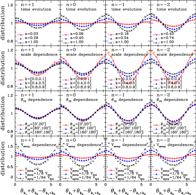
Figure 1 shows the time evolution, and the dependence on $k$, $\theta_{12}$ and $V_{\rm samp}$, of the distribution function of the phase sum (symbols) for scale-free models with power-law indices $n=-2$, $-1$, $0$, and $+1$. For comparison, we plot with lines the lowest-order analytic formula (eq.[6]) with $p^{(3)}$ directly evaluated from power spectra and bi-spectra of simulations. We note that the Poisson error of the distribution of the number of binned phase sum is very small.

Figure 1: Various parameter dependence of the distribution of the phase sum $\theta_{{\mbox{\scriptsize\boldmath$k$}}_{1}}+\theta_{{\mbox{\scriptsize\boldmath$k$}}_{2}}-\theta_{{\mbox{\scriptsize\boldmath$k$}}_{1}+{\mbox{\scriptsize\boldmath$k$}}_{2}}$ plotted by symbols in comparison with the perturbative formula (eq.[6]) plotted by lines for scale-free models. The power-law index $n$ decreases from left to right. Each panel shows the time evolution, the scale dependence, the $\theta_{12}$ dependence, and the sampling volume $V_{\rm samp}$ dependence from top to bottom.

Figure 2: Comparison of $p^{(3)}({\mbox{\boldmath$k$}}_{1},{\mbox{\boldmath$k$}}_{2})$ plotted by symbols with the amplitude of the distribution of phase sum at $\theta_{{\mbox{\scriptsize\boldmath$k$}}_{1}}+\theta_{{\mbox{\scriptsize\boldmath$k$}}_{2}}-\theta_{{\mbox{\scriptsize\boldmath$k$}}_{1}+{\mbox{\scriptsize\boldmath$k$}}_{2}}=0$ divided by the constant factor $\pi^{3/2}/4$ (see eq.[6]) plotted by lines for scale free models. The error-bars indicate the sample variances of $p^{(3)}$ and the amplitude of the distribution of phase sum for $n=-2$ model. Each panel shows the dependence of scale factor $a$ (Upper-Left), scale(Upper-Right), $\theta_{12}$ (Lower-Left) and sampling volume $V_{\rm samp}$ (Lower-Right).

Figure 3: Power spectrum $P(k)$ in units of $V_{\rm box}$ at various epochs in scale free models with $n=1$(Upper-left), $n=0$(Upper-right), $n=-1$(Lower-left) and $n=-2$(Lower-right).

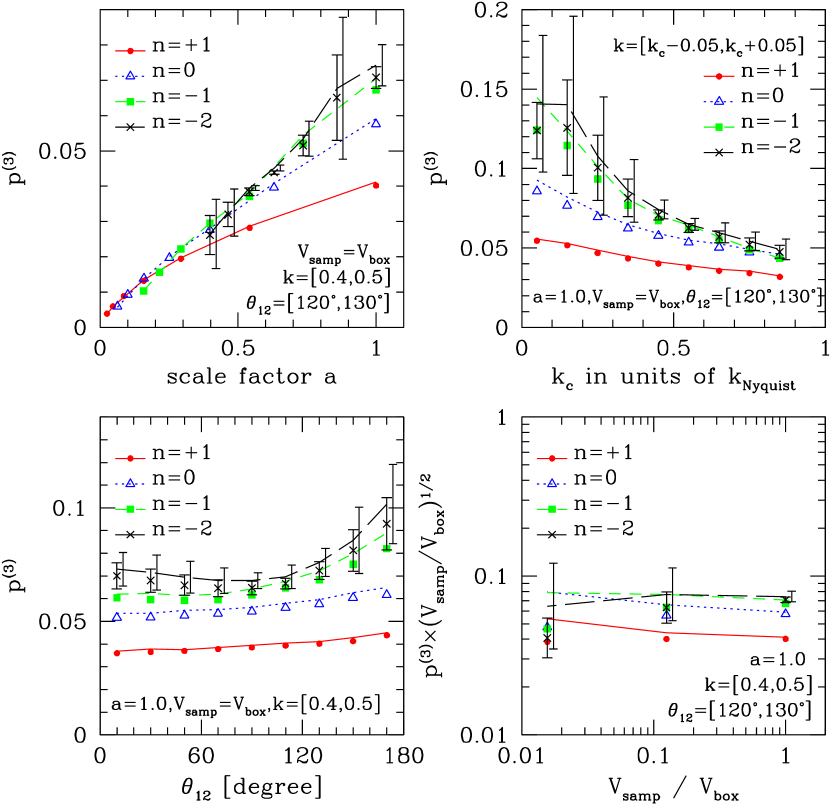
The symbols in Figure 2 plot the cumulant $p^{(3)}$ as a function of the scale factor $a$, the central value of the wavevector $k_{\rm c}$ ($k=[k_{\rm c}-0.05,k_{\rm c}+0.05]$), $\theta_{12}$, and $V_{\rm samp}$. The corresponding lines indicate $p^{(3)}$ evaluated from a fit of the phase-sum distribution to the analytic formula of equation (6). We choose the fitting range as $\theta_{{\mbox{\scriptsize\boldmath$k$}}_{1}}+\theta_{{\mbox{\scriptsize\boldmath$k$}}_{2}}-\theta_{{\mbox{\scriptsize\boldmath$k$}}_{1}+{\mbox{\scriptsize\boldmath$k$}}_{2}}=[1.9\pi,2\pi]$ and $[0\pi,0.1\pi]$ where the deviation from the lowest-order approximation is clearly seen. The quoted error-bars indicate the sample variance for $n=-2$ model.

Figures 1 and 2 employ a fiducial set of parameters, $a=1$, $k=[0.4,0.5]$, $\theta_{12}=[120^{\circ},130^{\circ}]$, and $V_{\rm samp}=V_{\rm box}$, except for one parameter that is examined in each panel.

The top panels in Figure 1 show the evolution of the PDF of the phase sum. In the earliest epochs, the density fields are still close to Gaussian and the PDF of the phase sum remains almost uniform. While the non-uniformity of the PDF develops at subsequent epochs, the upper-left panel in Figure 2 indicates that the lowest-order perturbation result well agrees with the simulation data even up to $a=1$.

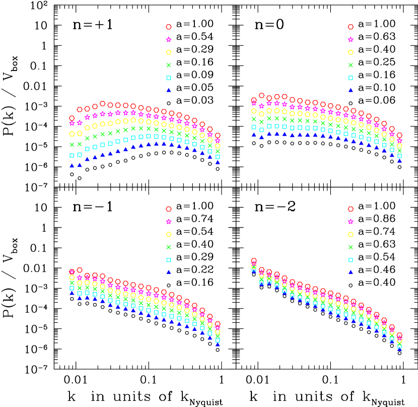
The second-upper panels in Figure 1 show the scale dependence of the phase-sum PDF. Again the overall agreement between the lowest-order perturbation theory and simulation data is very good. Nevertheless only on large scales ($k=[0.0,0.1]$), the lowest-order approximation starts to become invalid (see also the upper-right panel of Fig.2). The fluctuations on large scales should be closer to the linear stage, and thus this behavior seems to be inconsistent with a naive expectation that non-Gaussianity should show up first from small scales. This apparent discrepancy can be reconciled by the fact that the cumulant $p^{(3)}$ is approximately proportional to $\sqrt{P(k)/V_{\rm samp}}$ as we emphasized in §2. In all the current data of the scale-free models, the nonlinearly evolved power spectra $P(k)$ decrease with $k$ (Fig. 3). Therefore, as long as $V_{\rm samp}$ is fixed, $p^{(3)}$ is smaller for larger $k$, and thus the lowest-order perturbation provides a better approximation. This is an interesting and unique feature of the phase sum statistics that we examine here.

The second-lower panels in Figure 1 show the $\theta_{12}$ dependence of the phase-sum distribution. As indicated more clearly in the lower-left panel of Figure 2, the value of $p^{(3)}$, and thus the non-uniformity of the phase-sum PDF, increases slightly at $\theta_{12}\geq 120^{\circ}$ for $n=-1$ and $-2$ models. We suspect that this is ascribed to the presence of the large-scale filamentary structures in those models which the large $\theta_{12}$ (therefore small $|{\mbox{\boldmath$k$}}_{1}+{\mbox{\boldmath$k$}}_{2}|$) in $k$-space may correspond to.

The bottom panels in Figure 1 show the dependence on the sampling volume size $V_{\rm samp}$. Again unlike the conventional statistics, the PDF of the phase sum is indeed sensitive to the choice of $V_{\rm samp}$. The lower-right panel of Figure 2 illustrates that $p^{(3)}\sqrt{V_{\rm samp}}$ is approximately constant implying the validity of the hierarchical clustering ansatz as discussed in §2. This is why non-Gaussian feature of the PDF becomes substantially stronger and the higher-order terms become more important as $V_{\rm samp}$ becomes smaller.

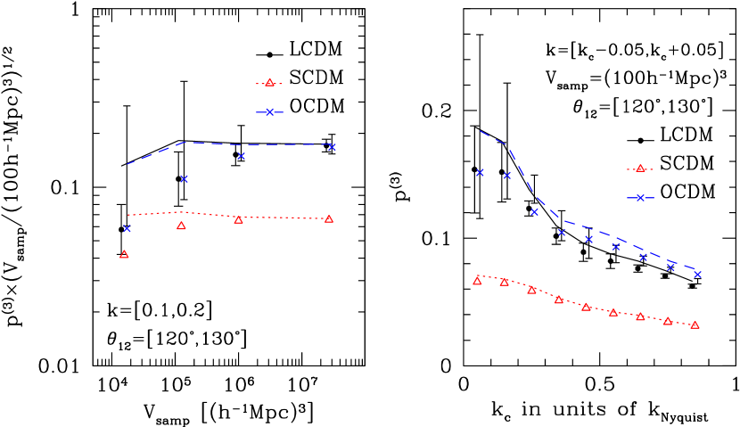
Figures 4 and 5 plot the same results as Figures 1 and 2 but for the CDM models. The distribution of the phase sum is more uniform in SCDM models compared with other models mainly due to the smaller value of $\sigma_{8}$ (Table 1). This is because the small $\sigma_{8}$ corresponds to the small power $P(k)$ with all over the scales and then $p^{(3)}\sim\sqrt{P(k)/V}$ has low value. The behavior of the parameter dependence is almost same as that in scale-free models. When a length of the simulation box is $300h^{-1}$Mpc, the lowest order approximation well agrees with simulations for any CDM models, while the approximation becomes worse as the box length decreases.

Figure 4: Comparison between the distribution of phase sum $\theta_{{\mbox{\scriptsize\boldmath$k$}}_{1}}+\theta_{{\mbox{\scriptsize\boldmath$k$}}_{2}}-\theta_{{\mbox{\scriptsize\boldmath$k$}}_{1}+{\mbox{\scriptsize\boldmath$k$}}_{2}}$ plotted by symbols and the lowest order perturbative equation (eq.[6]) plotted by lines for CDM models. The sampling volume $V_{\rm samp}$ is $(300h^{-1}{\rm Mpc})^{3}$, $(100h^{-1}{\rm Mpc})^{3}$, $(50h^{-1}{\rm Mpc})^{3}$, and $(25h^{-1}{\rm Mpc})^{3}$ from top to bottom. The range of the modulus $|{\mbox{\boldmath$k$}}_{1}|$ and $|{\mbox{\boldmath$k$}}_{2}|$ is $[0.1,0.2]$(open circles and solid lines), $[0.4,0.5]$(closed triangles and dotted lines), and $[0.8,0.9]$(crosses and dashed lines) in units of the Nyquist wavenumber $k_{\rm Nyquist}$ written in each panel.

Figure 5: Box-size and scale dependence of $p^{(3)}$ (symbols) in comparison with the amplitude of the distribution of the phase sum at $\theta_{{\mbox{\scriptsize\boldmath$k$}}_{1}}+\theta_{{\mbox{\scriptsize\boldmath$k$}}_{2}}-\theta_{{\mbox{\scriptsize\boldmath$k$}}_{1}+{\mbox{\scriptsize\boldmath$k$}}_{2}}=0$ normalized by the constant factor $\pi^{3/2}/4$ (lines) for CDM models. The error bars indicate the sample variance of $p^{(3)}$ and the amplitude of the distribution of the phase sum for LCDM model. Each panel shows the dependence of $V_{\rm samp}$ (Left) and $|{\mbox{\boldmath$k$}}_{1}|(|{\mbox{\boldmath$k$}}_{2}|)$ in units of $k_{\rm Nyquist}=2\pi/(0.78h^{-1}{\rm Mpc})$ (Right).

4.2 Correspondence between phase correlations and density peaks

As we emphasized over and over again, the PDF of the phase sum does depend on the size of the sampling volume. In order to understand the physical correspondence between the real-space distribution and the phase correlation, we compare the particle distribution from small sampling volumes on a sample-to-sample basis.

First note that the non-uniformity of the phase sum arises from a few dominating density peaks in the sampling volume. Consider a field which has just one spherical peak with a density profile $h(r)$ located at $\mbox{\boldmath$x$}_{0}$. The density field in this idealized system is given by $\rho(\mbox{\boldmath$x$})=h(|\mbox{\boldmath$x$}-\mbox{\boldmath$x$}_{0}|)$, and irrespective of the density profile of the peak, all the Fourier phases are aligned to $\theta_{\mbox{\scriptsize\boldmath$k$}}=-\mbox{\boldmath$k$}\cdot\mbox{\boldmath$x$}_{0}$. Thus the phase sum becomes zero in any combination of closed wavevectors. If another peak exists at a different position, the alignment of the phases is broken depending on the relative strength of the two peaks. If the peak height of the second peak is much smaller than that of the first, the phase alignment is almost preserved and the phase sum remains distributed around zero. On the other hand, if they have a comparable peak height, the phase alignment is significantly broken. In reality, all density peaks should contain substructure to some extent and many other structures in the field also contribute the eventual phase distribution. Nevertheless the above qualitative picture proves to be useful in understanding the physical meaning of the phase sum distribution.

Motivated by the above consideration, we examine in detail the connection between the particle distribution and the PDF of the phase sum. Figure 6 plots the projected particle distribution and the corresponding PDF of the phase sum for 8 different samples of ($25h^{-1}$Mpc)³ box from one of the LCDM simulations of ($100h^{-1}$Mpc)³ box.

After smoothing the particle distribution over the Gaussian window of $1h^{-1}$Mpc radius, we compute genus using CONTOUR 3D Weinberg (1988). Then we define the peak heights of the 1st, 2nd and 3rd peaks, $\delta_{1}$, $\delta_{2}$, and $\delta_{3}$ by the threshold density contrasts which the number of genus in the box changes from from $-1$ to $0$, from $-2$ to $-1$ and from $-3$ to $-2$, respectively. Those values are indicated in each panel of Figure 6. As expected from the above argument, Figure 6 clearly shows that the degree of non-uniformity of the PDF is related to the presence of the dominating peak in the box; the sample (d) has a single prominent density peak, and the phase sum is strongly distributed around zero, while the sample (b) has three almost comparable peaks resulting a fairly uniform PDF of the phase sum.

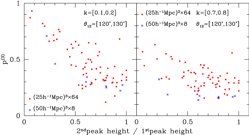
To be more quantitative, we compute $p^{(3)}$ and the ratio of the peak heights of the first and the second peaks for $64$ samples of $V_{\rm samp}=(25h^{-1}$Mpc)³ and $8$ samples of $V_{\rm samp}=(50h^{-1}$Mpc)³, both constructed from one realization of LCDM model. The result plotted in Figure 7 indeed supports the strong correlation between the value of $p^{(3)}$ and the ratio of the peak heights. In fact, this naturally explains the dependence of the PDF on $V_{\rm samp}$. As $V_{\rm samp}$ increases, the number of density peaks in the sampling volume increases and those peaks tend to weaken the correlation of the phase sum. This clearly illustrated in Figure 8 which plots the result for the box of $V_{\rm samp}=(50h^{-1}$Mpc)³ comprising all the eight samples of $V_{\rm samp}=(25h^{-1}$Mpc)³ plotted in Figure 6.

Figure 6: Comparison of the distribution of the phase sum with the value of three highest density peaks for eight fields with a box-length of $25h^{-1}$Mpc. The projected maps of dark matter particles are shown together. The distributions of the phase sum (symbols) are plotted together with the corresponding lowest order perturbative formula (lines) at three ranges of scale $|{\mbox{\boldmath$k$}}_{1}|$ and $|{\mbox{\boldmath$k$}}_{2}|$ in $[0.1,0.2]$ (filled circles, solid lines), $[0.4,0.5]$(open triangles, dotted lines) and $[0.7,0.8]$ (crosses, dashed lines) in units of $k_{\rm Nyquist}=2\pi/(0.78h^{-1}{\rm Mpc})$.

Figure 7: The relation between $p^{(3)}$ and the ratio of the second highest peak density to the highest peak density for the $64$ cubic data with a box-length of $25h^{-1}$Mpc (filled circles) and the $8$ cubic data with a box-length of $50h^{-1}$Mpc (crosses) based on LCDM cosmological model. The ranges of scale $|{\mbox{\boldmath$k$}}_{1}|$ and $|{\mbox{\boldmath$k$}}_{2}|$ are $[0.1,0.2]$ (Left) and $[0.7,0.8]$ (Right) in units of $k_{\rm Nyquist}=2\pi/(0.78h^{-1}{\rm Mpc})$ and $\theta_{12}=[120^{\circ},130^{\circ}]$.

Figure 8: Same as Figure 6 but for a box with a length of $50h^{-1}$Mpc constituted from the eight sub-boxes shown in Figure 6.

5 Conclusions and Discussion

We have performed a detailed numerical analysis of the phase correlation induced by nonlinear gravity in the universe. Following recent analytic work by Matsubara (2003b) in perturbation theory, we have computed the distribution function of the phase sum in triangle wavevectors and compared with his analytic formula. Using a large set of $N$-body simulations, we have explored the behavior of phase correlations for various configurations of wavevector triangles in the Fourier space at different epochs in a range of different sampling volumes. We find that the agreement of the simulations and the analytic perturbation formula is generally good.

Quite interestingly the series expansion of the analytic formula breaks down for $P(k)/V_{\rm samp}\sim 1$, which is in marked contrast to the conventional linear/nonlinear criterion, $P(k)k^{3}\sim 1$. Therefore the statistics of the phase sum indeed depends on the size of the sampling volume explicitly. This feature is naturally explained by the corresponding density structure in real space; all the phases are synchronized with each other when a distinctive density peak dominates in the given sampling volume, while the phase correlations become weaker if several peaks with comparable heights exist. We have confirmed this expectation directly by comparing the strength of phase correlations with the ratio of the highest peak to the secondary peaks in the sampling volume. Therefore the phase correlation becomes diluted as the sampling volume increases because statistically it accommodates a number of peaks with comparable heights.

The fact that the perturbation formula well reproduces the numerical results indicates that the information from the phase sum distribution mainly comes from the normalized bispectrum amplitude $p^{(3)}$. Since one can evaluate the bispectrum directly and independently from the phase sum distribution, one might wonder if the phase sum statistics is simply equivalent to the more conventional bispectrum analysis. Indeed the dependence on the sampling volume size may be a key in this context. This implies that any signal of non-Gaussianity in the phase correlation disappears in the large-volume limit. We can repeat the analysis by systematically decreasing the sampling volume size. Instead, one has to take an ensemble average of the phase correlations over many subsamples of a fixed $V_{\rm samp}$ to obtain proper statistical quantities. Otherwise, the phase correlations in a single volume is much like the cosmic variance, as the sharpness of the highest peak is weakened in the limit $V_{\rm samp}\rightarrow\infty$. The situation is similar to the count-in-cells statistics, as the exact number of the galaxies in a single cell is attributed to the cosmic variance. Taking an average of the weighted number in many cells gives a proper statistics, such as variance, skewness, kurtosis, and so forth. The average value and the sample variance with respect to the average as a function of $V_{\rm samp}$ may give additional information even beyond the bispectrum.

The distribution of the phase sum may be applied to the real data of the existing galaxy catalogues including the 2dF and SDSS, which provides complementary information beyond the two-point statistics. Since the phase sum statistics is a new concept in cosmology, we still need to explore many other aspects of the statistic that we are likely to have overlooked at this point. We are currently working on evaluating the phase-sum distributions of Sloan Digital Sky Survey galaxy samples considering all possible systematics by creating simulated Mock samples as we did in the previous topological analysis (Hikage et al. 2002, 2003). We hope to report the results elsewhere in near future.

Appendix A Box-size dependence of the cumulants $p^{(N)}$

According to the analytic formula of the joint PDF of arbitrary sets of the Fourier phase $\theta_{\mbox{\scriptsize\boldmath$k$}}$, the distribution of the phase sum is determined by the cumulants $p^{(N)}=\langle\alpha_{1}\alpha_{2}\cdots\alpha_{N}\rangle_{c}$ where $\alpha_{i}=f_{{\mbox{\scriptsize\boldmath$k$}}_{i}}/\sqrt{\langle|f_{{\mbox{\scriptsize\boldmath$k$}}_{i}}|^{2}\rangle}$ ($N\geq 3$ and $\langle\cdots\rangle$ denotes the spatial average). In this section, we present the relation of the cumulants $p^{(N)}$ to the power spectra and the polyspectra in physical unit (independent on the box-size) and explicitly show the dependence of $p^{(N)}$ on the box-size. First we give the definition of the power spectrum and the polyspectra and then apply it to the grid data.

In a three dimensional density fluctuation field $\delta({\mbox{\boldmath$x$}})=(\rho({\mbox{\boldmath$x$}})-\bar{\rho})/\bar{\rho}$, the Fourier-transform $\tilde{\delta}({\mbox{\boldmath$k$}})$ of $\delta({\mbox{\boldmath$x$}})$ in an infinite volume is given by

$$\tilde{f}({\mbox{\boldmath$k$}})=\int d^{3}x\delta({\mbox{\boldmath$x$}})e^{-i{\mbox{\scriptsize\boldmath$k$}}\cdot{\mbox{\scriptsize\boldmath$x$}}}.$$ (A1)

The polyspectra $P^{(N)}({\mbox{\boldmath$k$}}_{1},\cdot\cdot\cdot,{\mbox{\boldmath$k$}}_{N-1})$ are given by the cumulants

$$\left\langle\tilde{f}({\mbox{\boldmath$k$}}_{1})\cdots\tilde{f}({\mbox{\boldmath$k$}}_{N})\right\rangle_{c}=(2\pi)^{3}\delta_{D}^{3}({\mbox{\boldmath$k$}}_{1}+\cdot\cdot\cdot{\mbox{\boldmath$k$}}_{N})P^{(N)}({\mbox{\boldmath$k$}}_{1},\cdot\cdot\cdot,{\mbox{\boldmath$k$}}_{N-1}),$$ (A2)

where $\delta_{D}(\mbox{\boldmath$k$})$ is Dirac’s delta function. In this definition, the variance $\sigma^{2}=\langle\delta^{2}({\mbox{\boldmath$x$}})\rangle$ is given by

$$\sigma^{2}=\int\frac{k^{2}dk}{2\pi^{2}}P(k),$$ (A3)

where $P(|{\mbox{\boldmath$k$}}|)=P^{(2)}({\mbox{\boldmath$k$}})$ is the conventional power spectrum.

In a simulated box with a volume $V$ and a total grid number $N$, the lattice spacing of $x$ is $(V/N)^{1/3}$. In a lattice field $\delta({\mbox{\boldmath$x$}})$ with a discrete set of $x$’s, the discrete Fourier transform $f_{\mbox{\boldmath$k$}}$ is computed by

$$f_{\mbox{\scriptsize\boldmath$k$}}=\frac{\sqrt{V}}{N}\sum_{\mbox{\scriptsize\boldmath$x$}}\delta({\mbox{\boldmath$x$}})e^{-i{\mbox{\scriptsize\boldmath$k$}}\cdot{\mbox{\scriptsize\boldmath$x$}}},$$ (A4)

where the lattice spacing in $k$-space is $2\pi/V^{1/3}$. The correspondence between the discrete Fourier modes and the continuum Fourier modes is

$$\lim_{V\rightarrow\infty,V/N\rightarrow 0}\sqrt{V}f_{\mbox{\scriptsize\boldmath$k$}}=\tilde{f}({\mbox{\boldmath$k$}}).$$ (A5)

The cumulants $\left\langle f_{{\mbox{\scriptsize\boldmath$k$}}_{1}}\cdot\cdot\cdot f_{{\mbox{\scriptsize\boldmath$k$}}_{N}}\right\rangle_{c}$ are related to $P^{(N)}({\mbox{\boldmath$k$}}_{1},\cdot\cdot\cdot,{\mbox{\boldmath$k$}}_{N-1})$ by the relation

$$\left\langle f_{{\mbox{\scriptsize\boldmath$k$}}_{1}}\cdot\cdot\cdot f_{{\mbox{\scriptsize\boldmath$k$}}_{N}}\right\rangle_{c}=V^{1-N/2}\delta^{K}_{{\mbox{\scriptsize\boldmath$k$}}_{1}+\cdots+{\mbox{\scriptsize\boldmath$k$}}_{N}}P^{(N)}({\mbox{\boldmath$k$}}_{1},\cdot\cdot\cdot,{\mbox{\boldmath$k$}}_{N-1}),$$ (A6)

where $\delta^{K}_{\mbox{\scriptsize\boldmath$k$}}$ is Kronecker’s delta which is $1$ $({\mbox{\boldmath$k$}}=0)$ and $0$ $({\mbox{\boldmath$k$}}\neq 0)$. The correspondence between the Kronecker’s delta and the Dirac’s delta function is

$$\lim_{V\rightarrow\infty,V/N\rightarrow 0}V\delta^{K}_{\mbox{\scriptsize\boldmath$k$}}=(2\pi)^{3}\delta_{D}^{3}({\mbox{\boldmath$k$}}).$$ (A7)

The cumulants $p^{(N)}$ are, therefore, calculated by

$$p^{(N)} = \frac{\left\langle f_{{\mbox{\scriptsize\boldmath$k$}}_{1}}\cdot\cdot\cdot f_{{\mbox{\scriptsize\boldmath$k$}}_{N}}\right\rangle_{c}}{\sqrt{\langle|f_{{\mbox{\scriptsize\boldmath$k$}}_{1}}|^{2}\rangle\cdot\cdot\cdot\langle|f_{{\mbox{\scriptsize\boldmath$k$}}_{N}}|^{2}\rangle}}$$ (A8)

$$= \frac{P^{(N)}({\mbox{\boldmath$k$}}_{1},\cdot\cdot\cdot,{\mbox{\boldmath$k$}}_{N-1})}{\sqrt{V^{N-2}P({\mbox{\boldmath$k$}}_{1})\cdot\cdot\cdot P({\mbox{\boldmath$k$}}_{N})}}.$$

The box-size dependence of $p^{(N)}\propto V^{1-N/2}$ means that higher order terms become dominant as the box-size decreases even when $k^{3}P(k)$ is small.

References

- Bardeen et al. (1986) Bardeen, J. M., Bond, J. R., Kaiser, N., & Szalay, A. S. 1986, ApJ, 304, 15
- Bertschinger (1992) Bertschinger, E., in Lecture Notes in Physics, 408, New Insights into the Universe, ed. Martinez, V. J., Portilla, M., & Saez, D., p65 (Springer-Verlag, Berlin, 1992)
- Chiang (2001) Chiang, L. 2001, MNRAS, 325, 405
- Chiang et al. (2002) Chiang, L., Coles, P., & Naselsky, P. D. 2002, MNRAS, 337, 488
- Coles & Chiang (2000) Coles, P., & Chiang, L. 2000, Nature, 406, 376
- Gott et al. (1986) Gott III, J. R., Mellot, A. L., & Dickinson, M. 1986, ApJ, 306, 341
- Hikage et al. (2002) Hikage, C., Suto, Y., Kayo, I., Taruya, A., Matsubara, T., Vogeley, M. S., Hoyle, F., Gott, J. R., III, & Brinkmann, J., for the SDSS collaboration 2002, PASJ, 54, 707
- Hikage et al. (2003) Hikage, C., Schmalzing, J., Buchert, T., Suto, Y., Kayo, I., Taruya, A., Vogeley, M. S., Hoyle, F., Gott, J. R., III, & Brinkmann, J., for the SDSS collaboration 2003, PASJ, 55, in press.
- Jain & Bertschinger (1998) Jain, B., & Bertschinger, E. 1998, ApJ, 509, 517
- Jing (1998) Jing, Y. P. 1998, ApJ, 503, L9
- Jing & Suto (1998) Jing, Y. P., & Suto, Y. 1998, ApJ, 494, L5
- Matsubara (1995) Matsubara, T. 1995, ApJS, 101, 1
- (13) Matsubara, T. 2003a, ApJ, 584, 1
- (14) Matsubara, T. 2003b, ApJL, 591, L79
- Mecke et al. (1994) Mecke, K. R., Buchert, T., & Wagner, H. 1994, A&A, 288, 697
- Ryden & Gramann (1991) Ryden, B. S., & Gramann, M. 1991, ApJ, 383, L33
- Scherrer et al. (1991) Scherrer, R. J., Melott, A. L., & Shandarin, S. F. 1991, ApJ, 377, 29
- Schmalzing & Buchert (1997) Schmalzing, J., & Buchert, T. 1997, ApJ, 482, L1
- Soda & Suto (1992) Soda, J., & Suto, Y. 1992, ApJ, 396, 379
- Suginohara & Suto (1991) Suginohara, T., & Suto, Y. 1991, ApJ, 371, 470
- Watts & Coles (2003) Watts, P., & Coles, P. 2003, MNRAS, 338, 806
- Watts et al. (2003) Watts, P., Coles, P., & Melott, A. 2003, ApJ, 589, L61
- Weinberg (1988) Weinberg, D. H. 1988, PASP, 100, 1373
- White (1979) White, S. D. M. 1979, MNRAS, 186, 145