The relation between the two-point and the three-point correlation functions in the non-linear gravitational clustering regime

Abstract

The connection between the two-point and the three-point correlation functions in the non-linear gravitational clustering regime is studied. Under a scaling hypothesis, we find that the three-point correlation function, $\zeta$, obeys the scaling law $\zeta\propto\xi^{\frac{3m+4w-2\epsilon}{2m+2w}}$ in the nonlinear regime, where $\xi$, $m$, $w$, and $\epsilon$ are the two-point correlation function, the power index of the power spectrum in the nonlinear regime, the number of spatial dimensions, and the power index of the phase correlations, respectively. The new formula reveals the origin of the power index of the three-point correlation function. We also obtain the theoretical condition for which the “hierarchical form” $\zeta\propto\xi^{2}$ is reproduced.

1 Introduction

The formation of large-scale structures in the Universe is one of the most important and interesting problems in cosmology. It is generally believed that these structures have developed by a process of gravitational instability from small initial fluctuations in the density of a largely homogeneous early Universe. Hence it is very important to clarify the physical mechanism of the evolution of density fluctuations. Here we consider the density fluctuations of collisionless particles, such as dark matter, because our interest is concentrated on the effects of self-gravity.

The inflationary scenario predicts a random Gaussian field possessing the properties of statistical homogeneity and isotropy as the primordial fluctuations (Guth, 1981; Guth & Pi, 1982; Bardeen et.al., 1986). The statistical properties of the Gaussian field are completely characterized by the two-point correlation function (hereafter 2PCF) or the power spectrum, since higher order correlations vanish, while only the 2PCF has a certain value (Adler, 1981). However, non-linear gravitational clustering gives rise to non-zero values of the higher-order correlations, even if the primordial density fluctuations were set Gaussian. This is reasonable, since phases between Fourier modes in the bispectrum are considered to be distributed non-randomly but correlated in some ways in the non-linear regime, where galaxies or galaxy groups are strongly clustered around each other (Scherrer, Melott & Shandarin, 1991; Coles & Chiang, 2000; Chiang, 2001; Chiang, Naselsky & Coles, 2002; Watts & Coles, 2003; Watts, Coles & Melott, 2003; Matsubara, 2003). Hence the higher order statistics, like the three-point correlation function (hereafter 3PCF), become essential when the evolution of the density fields is governed by non-linear gravitational clustering. So it is quite important for understanding non-linear evolution to investigate the properties of the 3PCF.

Generally, it is hard to deal with the exact formula of the 3PCF both theoretically and numerically, since it is much more lengthy and complicated than 2PCF. Historically, however, Peebles & Groth (1975); Groth & Peebles (1977) had proposed a simple assumption: the 3PCF can be expressed by the product of the 2PCF as

$$\zeta_{abc}=Q[\xi_{ab}\xi_{bc}+\xi_{bc}\xi_{ca}+\xi_{ca}\xi_{ab}],$$ (1)

where $\zeta$, $\xi$, and $Q$ are the 3PCF, the 2PCF, and a certain constant, respectively. The expression (1) or $\zeta\propto\xi^{2}$ is often called the “hierarchical form” (Fry, 1984). The data from the Zwicky and Shane-Wirtanen catalogs are in good agreement with this assumption when we choose $Q\simeq 0.85$ for Zwicky and $Q\simeq 1.24$ for Shane-Wirtanen (Peebles & Groth, 1975; Groth & Peebles, 1977).

However, there is a serious fault with the proposal (1). It has no theoretical ground, although some observational or numerical data may be well-fitted. One explanation may be that Eq. (1) for $\zeta$ with $Q=1$ coincides with the Kirkwood superposition approximation which is familiar in liquid physics and turbulence theory, if $\xi_{ab}\xi_{bc}\xi_{ca}\ll 1$ (Davies & Peebles, 1977; Ichimaru, 1973). However, this approximation is not appropriate for the non-linear regime, since the distribution of the gravitational sources is strongly correlated, $\xi\gg 1$, in such regimes. Hence this resemblance is helpless to compensate for the theoretical defect.

Indeed, there were many theoretical investigations of the 3PCF (Fry, 1984; Ruamsuwan & Fry, 1992). Nevertheless most of the analyses have been based on the “hierarchical form” assumption. The coefficient $Q$ under the “hierarchical form” was estimated by assuming self-similarity (Fry, 1984). The BBGKY hierarchy was analyzed by assuming the “hierarchical form” as well as self-similarity (Ruamsuwan & Fry, 1992). In the first place, however, there is no reason why the 3PCF should necessarily depend only on the second power of the 2PCF, even if we accept the self-similarity. Indeed, Yano & Gouda (1997) suggests the possible existence of solutions that do not satisfy the “hierarchical form” on the basis of the BBGKY equations. Therefore an investigation of the physical adequacy of the “hierarchical form” itself and more reliable and useful formulae for the 3PCF are pressingly required.

In this paper we study the connection between the 2PCF and the 3PCF in the non-linear gravitational clustering regime. We analyze these functions using a scaling hypothesis. It is expected that the time evolution of the statistics obeys also some self-similar rules fundamentally, since gravity is scale free (Davies & Peebles, 1977; Fry, 1984; Ruamsuwan & Fry, 1992; Yano & Gouda, 1998). Many authors have investigated the self-similarity of the 2PCF or the power spectrum. Recent works using N-body simulations (Colombi, Bouchet, & Hernquist, 1996; Couchman & Peebles, 1997; Jain, Mo & White, 1995) have shown that self-similar evolution of the power spectrum can be satisfied when the initial power spectrum is scale free, and the power spectrum in the non-linear regime obeys some scaling laws. The scaling hypothesis itself is very familiar. However, the unique proposition in this paper is that we apply the scaling hypothesis to the bispectrum as well as to the power spectrum, and we never assume the “hierarchical form”. Consequently, we succeed in deriving a new formula for the 3PCF, focusing on the power indices. The relevance to the “hierarchical form” is also discussed.

Our paper is organized as follows. In Sec.2 we introduce the general formula of the 2PCF and the 3PCF. We obtain in Sec.3 a new relationship between these functions the under the scaling hypothesis. In Sec.4 we calculate the 2PCF and the 3PCF in the non-linear regime in the one-dimensional Einstein-de Sitter model numerically, in order to confirm the analytical results. The final section is devoted to summary.

2 General formula for the correlation functions

In this section we consider the 2PCF and the 3PCF. Let us denote by $\bar{\rho}$ the mean density and take $\rho({\mbox{\boldmath$x$}})$ to be the density at a point specified by the position vector $x$ with respect to some arbitrary origin. As usual, we define the fluctuation to be

$$\delta({\mbox{\boldmath$x$}})=\frac{\rho({\mbox{\boldmath$x$}})-\bar{\rho}}{\bar{\rho}}.$$ (2)

We assume this to be expressible as a Fourier series:

$$\delta_{{\mbox{\boldmath$k$}}}=\frac{1}{L^{w}}\int\delta({\mbox{\boldmath$x$}})e^{i{\mbox{\boldmath$k$}}\cdot{\mbox{\boldmath$x$}}}d^{w}x,$$ (3)

and

$$\delta({\mbox{\boldmath$x$}})=\frac{L^{w}}{(2\pi)^{w}}\int\delta_{{\mbox{\boldmath$k$}}}e^{-i{\mbox{\boldmath$k$}}\cdot{\mbox{\boldmath$x$}}}d^{w}k,$$ (4)

where $\delta_{{\mbox{\boldmath$k$}}}$, $w$ and $L$ are a Fourier amplitude, the number of the spatial dimensions, and the length of the side of the box, respectively. The 2PCF is defined in terms of the density fluctuation by

$$\xi({\mbox{\boldmath$r$}}) = \left\langle\left\langle\delta({\mbox{\boldmath$x$}})\delta({\mbox{\boldmath$x$}}+{\mbox{\boldmath$r$}})\right\rangle_{{\mbox{\boldmath$x$}}}\right\rangle$$ (5)

$$= \left\langle\left\langle\frac{L^{2w}}{(2\pi)^{2w}}\iint\delta_{{\mbox{\boldmath$k$}}}\delta_{{\mbox{\boldmath$k^{\prime}$}}}e^{-i({\mbox{\boldmath$k$}}+{\mbox{\boldmath$k^{\prime}$}})}\cdot{\mbox{\boldmath$x$}}e^{-i{\mbox{\boldmath$k$}}\cdot{\mbox{\boldmath$r$}}}d^{w}kd^{w}k^{\prime}\right\rangle_{{\mbox{\boldmath$x$}}}\right\rangle,$$

where the angular brackets in Eq.(5) are expectation values, formally denoting an average over the probability distribution of $\delta({\mbox{\boldmath$x$}})$. The first average, $\langle\quad\rangle_{{\mbox{\boldmath$x$}}}$, means simply a volume normalization over a sufficiently large patch of the Universe. The second average, $\langle\quad\rangle$, is interpreted as that across independent samples in many Universes. Applying this rule and performing the volume integration gives

$$\xi({\mbox{\boldmath$r$}}) = \frac{L^{w}}{(2\pi)^{w}}\iint\langle\delta_{{\mbox{\boldmath$k$}}}\delta_{{\mbox{\boldmath$k^{\prime}$}}}\rangle\delta_{D}({\mbox{\boldmath$k$}}+{\mbox{\boldmath$k^{\prime}$}})e^{-i{\mbox{\boldmath$k$}}\cdot{\mbox{\boldmath$r$}}}d^{w}k^{\prime}d^{w}k$$ (6)

$$\equiv \frac{L^{w}}{(2\pi)^{w}}\int P({\mbox{\boldmath$k$}})e^{-i{\mbox{\boldmath$k$}}\cdot{\mbox{\boldmath$r$}}}d^{w}k,$$

where $\delta_{D}$ is the Dirac delta-function and $P({\mbox{\boldmath$k$}})$ is the power spectrum. Similarly, it is possible to calculate the 3PCF, which is defined as

$$\zeta({\mbox{\boldmath$r$}},{\mbox{\boldmath$s$}}) = \langle\langle\delta({\mbox{\boldmath$x$}})\delta({\mbox{\boldmath$x$}}+{\mbox{\boldmath$r$}})\delta({\mbox{\boldmath$x$}}+{\mbox{\boldmath$s$}})\rangle_{{\mbox{\boldmath$x$}}}\rangle$$ (7)

$$= \left\langle\left\langle\frac{L^{3w}}{(2\pi)^{3w}}\iiint\delta_{{\mbox{\boldmath$k$}}}\delta_{{\mbox{\boldmath$k^{\prime}$}}}\delta_{{\mbox{\boldmath$k^{\prime\prime}$}}}e^{-i({\mbox{\boldmath$k$}}+{\mbox{\boldmath$k^{\prime}$}}+{\mbox{\boldmath$k^{\prime\prime}$}})\cdot{\mbox{\boldmath$x$}}}e^{-i({\mbox{\boldmath$k$}}\cdot{\mbox{\boldmath$r$}}+{\mbox{\boldmath$k^{\prime}$}}\cdot{\mbox{\boldmath$s$}})}d^{w}kd^{w}k^{\prime}d^{w}k^{\prime\prime}\right\rangle_{{\mbox{\boldmath$x$}}}\right\rangle.$$

The volume integration gives

$$\zeta({\mbox{\boldmath$r$}},{\mbox{\boldmath$s$}}) = \frac{L^{2w}}{(2\pi)^{2w}}\iiint\langle\delta_{{\mbox{\boldmath$k$}}}\delta_{{\mbox{\boldmath$k^{\prime}$}}}\delta_{{\mbox{\boldmath$k^{\prime\prime}$}}}\rangle\delta_{D}({\mbox{\boldmath$k$}}+{\mbox{\boldmath$k^{\prime}$}}+{\mbox{\boldmath$k^{\prime\prime}$}})e^{-i({\mbox{\boldmath$k$}}\cdot{\mbox{\boldmath$r$}}+{\mbox{\boldmath$k^{\prime}$}}\cdot{\mbox{\boldmath$s$}})}d^{w}kd^{w}k^{\prime}d^{w}k^{\prime\prime}$$ (8)

$$= \frac{L^{2w}}{(2\pi)^{2w}}\iint\langle\delta_{{\mbox{\boldmath$k$}}}\delta_{{\mbox{\boldmath$k^{\prime}$}}}\delta_{-{\mbox{\boldmath$k$}}-{\mbox{\boldmath$k^{\prime}$}}}\rangle e^{-i({\mbox{\boldmath$k$}}\cdot{\mbox{\boldmath$r$}}+{\mbox{\boldmath$k^{\prime}$}}\cdot{\mbox{\boldmath$s$}})}d^{w}kd^{w}k^{\prime}$$

$$\equiv \frac{L^{2w}}{(2\pi)^{2w}}\iint B({\mbox{\boldmath$k$}},{\mbox{\boldmath$k^{\prime}$}})e^{-i({\mbox{\boldmath$k$}}\cdot{\mbox{\boldmath$r$}}+{\mbox{\boldmath$k^{\prime}$}}\cdot{\mbox{\boldmath$s$}})}d^{w}kd^{w}k^{\prime},$$

where $B({\mbox{\boldmath$k$}},{\mbox{\boldmath$k^{\prime}$}})$ is the bispectrum (Fry, 1984). The volume integration gives rise to the triangular constraint by the Dirac delta-function, which is similar to Eq.(6) (see also Fry (1984); Watts & Coles (2003); Matsubara (2003)).

3 The connection between the 2PCF and the 3PCF under the scaling hypothesis

In this section we derive the connection between the 2PCF and the 3PCF, under the scaling hypothesis. This assumption is adequate, since we consider that fluctuations evolve purely due to gravity. First, we assume that the power spectrum in the non-linear regime obeys a power law as

$$P(k) = \langle|\delta_{k}|^{2}\rangle$$ (9)

$$\propto k^{m},$$

where the index is a value in the non-linear regime. Substituting Eq.(9) into Eq.(6) gives

$$\xi(r) \propto \int k^{m}d^{w}k$$ (10)

$$\propto r^{-(m+w)}.$$

Next, the bispectrum in Eq.(8) is decomposed by

$$B(k,k^{\prime})=\left\langle|\delta_{k}||\delta_{k^{\prime}}||\delta_{-k-k^{\prime}}|e^{i(\phi_{k}+\phi_{k^{\prime}}+\phi_{-k-k^{\prime}})}\right\rangle,$$ (11)

where $\phi_{k}$ is the Fourier phase of the modes with wave number $k$. Now we consider the Fourier phases in Eq.(11) in the non-linear regime. Let us consider that the initial fluctuations are a random Gaussian field whose phases are distributed randomly. Induced by the gravitational instability, however, the density fluctuations become stronger and stronger, which means the phases between Fourier modes become distributed non-randomly (Scherrer, Melott & Shandarin, 1991; Coles & Chiang, 2000; Chiang, 2001; Chiang, Naselsky & Coles, 2002; Watts & Coles, 2003; Watts, Coles & Melott, 2003). That is, the Fourier phases are also correlated due to the gravitational clustering. It is not difficult to imagine that the phases synchronize in the case of the gravitational collapse, like a pancake, for example.

Generally, the 3PCF or the bispectrum depends on the shape of the configuration. If we fix the shape of the triangle, however, the 3PCF and the bispectrum are determined by one parameter. Here we assume the bispectrum in the strong non-linear regime obeys a scaling law as well as the power spectrum. Hence the expectation value of the Fourier phase in the bispectrum (11) is described as

$$\langle e^{i(\phi_{kt}+\phi_{k^{\prime}t}+\phi_{-kt-k^{\prime}t})}\rangle\propto t^{-\alpha}\langle e^{i(\phi_{k}+\phi_{k^{\prime}}+\phi_{-k-k^{\prime}})}\rangle$$ (12)

in the strongly non-linear regime. The scaling hypothesis for the Fourier phases corresponds to the following two characteristic possibilities physically: first, the Fourier phases remain correlated, and the expectation value converges to some non-zero constant value through non-linear gravitational clustering. In this case the value of $\alpha$ in Eq.(12) is zero. Second, the Fourier phase correlations are finally relaxed due to non-linear gravitational clustering, although the phases may be correlated once by gravitational instability. In this case the expectation value of the Fourier-phase correlations converges to zero, and the value of $\alpha$ in Eq.(12) is some finite value that depends on the degree of convergence. That is, the constant $\alpha$ should be a non-negative value. Similarly, other terms in Eq.(11) are also assumed to obey some scaling laws (For a detailed description, see Appendix A).

From Appendix A, the 3PCF is reduced to

$$\zeta(r,s) \propto \iint B(k,k^{\prime})d^{w}kd^{w}k^{\prime}$$ (13)

$$\propto t^{-(\frac{3}{2}m+2w-\alpha)}\iint\langle|\delta_{tk}|\rangle\langle|\delta_{tk^{\prime}}|\rangle\langle|\delta_{-tk-tk^{\prime}}|\rangle\langle e^{i(\phi_{tk}+\phi_{tk^{\prime}}+\phi_{-tk-tk^{\prime}})}\rangle d^{w}(tk)d^{w}(tk^{\prime})$$

$$+t^{-(\frac{3}{2}m+2w-\beta-\gamma_{4y})}\iint\langle|\delta_{tk}|\rangle\langle|\delta_{tk^{\prime}}|\rangle\langle|\delta_{-tk-tk^{\prime}}|\rangle\langle\delta e^{i(\phi_{tk}+\phi_{tk^{\prime}}+\phi_{-tk-tk^{\prime}})}\rangle d^{w}(tk)d^{w}(tk^{\prime})$$

$$+\cdots.$$

Where $\beta$ and $\gamma$ are the scaling factors of variance and other constants. It is noting that each value of these factors should be non-negative so that the 3PCF should not diverge. Then the 3PCF can be approximated by

$$\zeta(r,s) \propto t^{-(\frac{3}{2}m+2w-\epsilon)}\zeta\left(\frac{r}{t},\frac{s}{t}\right),$$ (14)

that is,

$$\zeta(r)\propto r^{-(\frac{3}{2}m+2w-\epsilon)},$$ (15)

where $\epsilon$ is defined as

$$\epsilon\equiv min(\alpha,\>\beta+\gamma_{2y},\>\beta+\gamma_{3y},\>\beta+\gamma_{4y}).$$ (16)

From Eqs.(10) and (15), we obtain a new expression to connect between $\zeta$ and $\xi$ as

$$\zeta\propto\xi^{\frac{3m+4w-2\epsilon}{2m+2w}}.$$ (17)

The proportional expression (17) states that the 3PCF is proportional to the power of the 2PCF. The power index depends on the power index of the power spectrum in the non-linear regime, $m$, and the scaling factors of the bispectrum, $\epsilon$. The formula clarifies the source of the power index of the 3PCF under the scaling hypothesis.

Now we consider the case $\alpha\neq 0$, where the phase the phase correlations get loose by the non-linear gravitational clustering, although they are tied tight once. Still the information of the convergence survives in the power index of the formula (17) . We can know the power index of the 3PCF by calculating the power index of the power spectrum and the phase correlation in the bispectrum (11). In particular, if the equality $\epsilon=-m/2$ is satisfied, the “hierarchical form”, $\zeta\propto\xi^{2}$, can be reproduced. For example, we consider the case $\xi\propto r^{-1.8}$ [Davies&Peebles 1977]. In this case, the index $m$ is equal to $-1.2$, and our formula agrees to the “hierarchical form”, if $\epsilon=0.6$.

Next, we consider the case where the Fourier phases keep correlated through the non-linear effects. In this case the expectation value of the phase correlations converges to a finite constant value, $\alpha=0$. Then the power index of the formula (17) depends only on the index of the power spectrum and the number of the spatial dimension,

$$\zeta\propto\xi^{\frac{3m+4w}{2m+2w}}.$$ (18)

Accordingly, the 3PCF can be described as the closed form only by the 2PCF. As a typical example, it is expected that the relation is realized at the moment of the gravitational collapse into a pancake, since the phases are synchronized strongly. In addition, if the power index of the power spectrum is zero, $m=0$, the 3PCF is proportional to the second power of the 2PCF. Recall that the index of the power spectrum is around zero in the transitional region from the linear regime to the non-linear regime, if the power index of the power spectrum of the initial random Gaussian field is not negative value. Considering these facts, we suppose the “hierarchical form” might be also realized accidentally around such quasi-linear scales.

4 Numerical test in the one-dimensional model

In this section we demonstrate the numerical simulation by the one-dimensional model to confirm our analytical expression. This model enables us to simulate with high accuracy, since the numerical errors of the algorithm include only round-off errors. Here we investigate the time evolution of a plane–symmetric density perturbation in an Einstein–de Sitter universe model by using a semi–analytical method. In the one–dimensional system many plane–parallel sheets move only in perpendicular direction to the surface of these sheets. When two sheets cross, they are allowed to pass through each other freely. In this sheet system, there is an exact solution until two sheets cross over as follows (Zel’dovich, 1970; Sunyaev & Zel’dovich, 1972; Doroshkevich et al., 1973; Zentsova & Chernin, 1980; Yano & Gouda, 1998):

$$x = q+B_{1}(t)S_{1}(q)+B_{2}(t)S_{2}(q),$$

$$v = \dot{B_{1}}(t)S_{1}(q)+\dot{B_{2}}(t)S_{2}(q)\;\;,$$ (19)

where $q$ and $x$ are the Lagrangian and the (comoving) Eulerian coordinates, respectively. Here, $S_{1}(q)$, and $S_{2}(q)$ are arbitrary functions of $q$. $B_{1}(t)$, and $B_{2}(t)$ are the growing mode and the decaying mode of linear perturbation solutions, respectively. We are considering the Einstein–de Sitter background universe model, i.e., $B_{1}(t)=a$ and $B_{2}(t)=a^{-\frac{3}{2}}$, where $a$ is the scale factor. The velocity $v$ is the peculiar–velocity normalized by the scale factor. We can compute the crossing time of all neighboring pairs of sheets. We use the shortest of these crossing times as a time step. Then, we can compute the new positions and velocities for all sheets at this crossing time. After two sheets cross, we exchange the velocities of the two sheets that just crossed. Then we obtain again $S_{1}(q),S_{2}(q)$, and therefore the exact solutions as follows:

$$S_{1}(q)=\frac{3}{5}a^{-1}(x-q)+\frac{2}{5}\dot{a}^{-1}v,$$

$$S_{2}(q)=\frac{2}{5}a^{\frac{3}{2}}(x-q)-\frac{2}{5}\dot{a}^{-1}a^{\frac{5}{2}}v\;\;.$$ (20)

These new exact solutions can be used until again two sheets cross. In this way we obtain the exact loci of the sheets by coupling these solutions. This semi–analytic method has good accuracy, because we connect exact solutions.

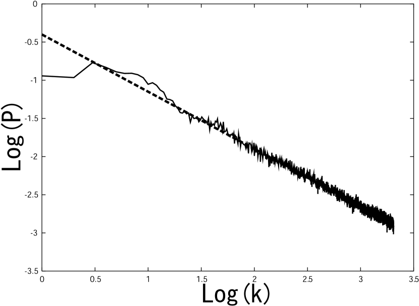
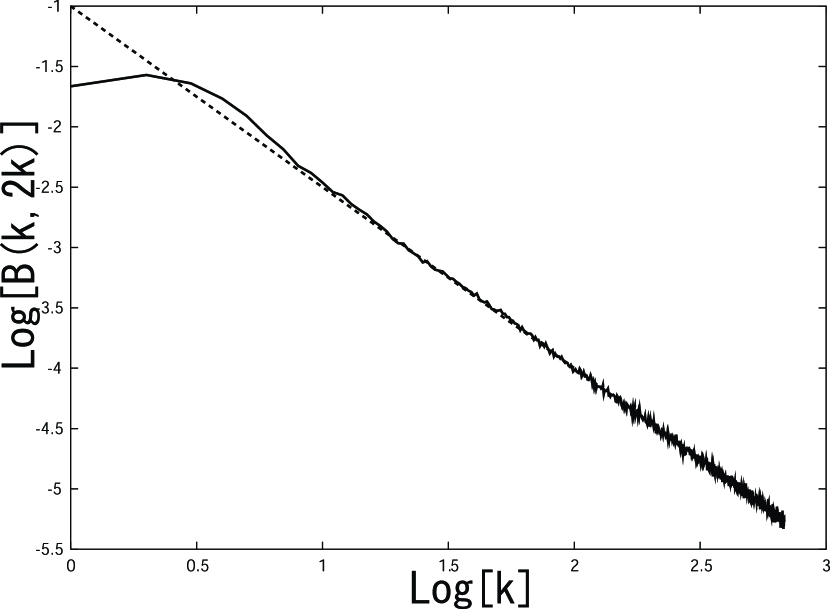
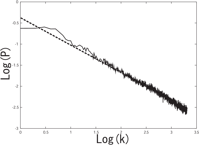
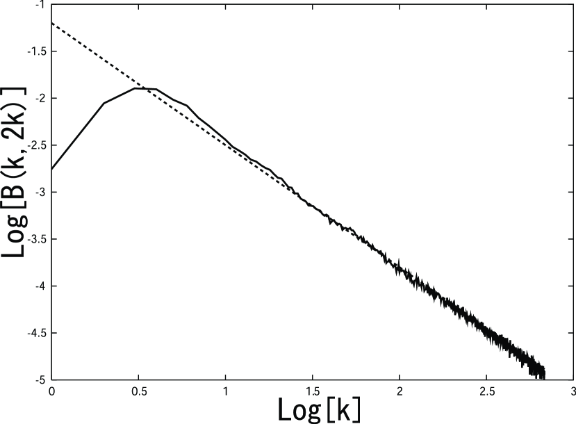
In our calculation we are going to use $2^{12}$ sheets. Periodic boundary conditions are fixed at a length of $2$. Here we consider the time evolution from a random-Gaussian initial condition with the index of the power spectrum given by $1$ or $2$. The shape of the triangle is chosen as $r=2s$. In addition, we take the ensemble average over 100 samples. Figure 1 shows the power spectrum in the nonlinear gravitational regime where we have chosen the initial power index $1$. It can be fitted by $P(k)\propto k^{-0.75}$, which agrees with Yano & Gouda (1998). From the Fourier transform, the 2PCF obeys $\xi(r)\propto r^{-0.25}$. Figure 2 shows the bispectrum in the nonlinear regime when the power spectrum is expressed as in Figure 1. It is obvious that the bispectrum is well fitted by $B(k,2k)\propto k^{-1.5}$. Similarly, Figure 4 shows the bispectrum in the nonlinear regime when the power spectrum is expressed as in Figure 3. It is obvious that the bispectrum is well fitted by $B(k,2k)\propto k^{-1.3}$. These value agree with $B(k,2k)\propto k^{2m}$, which is predicted by expression (17) with the relation $\epsilon=-m/2$. In other words, these results agree with the hierarchical assumption $\zeta\propto\xi^{2}$.

5 Summary

In this paper we have studied the connection between the 2PCF and the 3PCF in the non-linear gravitational clustering regime. Under the scaling hypothesis to the bispectrum as well as the power spectrum, we have derived a new formula regarding the 3PCF. It is striking that the origin of the power index of the 3PCF has been revealed. Moreover we have checked the validity of the analytical expression using numerical simulations in the one-dimensional Einstein-de Sitter model.

Under the scaling hypothesis, we have obtained the connection (17), in which there remain two characteristic possibilities for evolution of the phases of the Fourier modes: they remain correlated or tend to become uncorrelated in the strongly non-linear regime. Expression (17) states that the power index of the 3PCF generally consists of information from the third-order statistics, $\epsilon$, as well as that from the 2PCF.

It is generally believed that the power index of the power spectrum in the non-linear regime, $m$, is decided by the initial power spectrum. Combining this fact and our formula, Eq. (17), we can claim that the power index of the 3PCF originates from the initial power spectrum. Therefore, it will be important future work to clarify the relationship between the power spectrum in the non-linear regime and the initial one. Furthermore, the confirmation of the scaling of the 3PCF in three-dimensional N-body simulations is very important future work, although it is much more difficult to calculate the 3PCF in three-dimensional space than in one-dimensional.

The radical progress of recent observations needs increasingly advanced and practical formalism for analyses containing the higher-order statistics. Hence our new formula is expected to be a good indicator to understand the non-linear gravitational clustering. For this purpose it will be a subsequent task to check if the new formula is consistent with the BBGKY hierarchy. In addition, it will also be important to complete the formula by investigating the coefficients as well as the power indices in order to inspect the adjustment with the “hierarchical form” and to understand the physical origin of $Q$. We hope the new formula becomes a very useful instrument for analysis of large-scale structure.

Appendix A Bispectrum under the scaling hypothesis

Firstly we decompose the absolute value of the Fourier spectrum of density fluctuation and the Fourier phase into their averages and the discrepancies:

$$X_{a}=\langle X_{a}\rangle+\delta X_{a}=|\delta_{tk}|,$$ (A1)

$$X_{b}=\langle X_{b}\rangle+\delta X_{b}=|\delta_{tk^{\prime}}|,$$ (A2)

$$X_{c}=\langle X_{c}\rangle+\delta X_{c}=|\delta_{-tk-tk^{\prime}}|,$$ (A3)

$$Y=\langle Y\rangle+\delta Y=e^{i(\phi_{tk}+\phi_{tk^{\prime}}+\phi_{-tk-tk^{\prime}})}.$$ (A4)

Then the bispectrum is rewritten by

$$B(tk,tk^{\prime})=\left\langle X_{a}X_{b}X_{c}Y\right\rangle = \left\langle(\langle X_{a}\rangle+\delta X_{a})(\langle X_{b}\rangle+\delta X_{b})(\langle X_{c}\rangle+\delta X_{c})(\langle Y\rangle+\delta Y)\right\rangle$$ (A5)

$$= \langle X_{a}\rangle\langle X_{b}\rangle\langle X_{c}\rangle\langle Y\rangle+\langle X_{a}\rangle\langle X_{b}\rangle\langle X_{c}\rangle\left\langle\delta Y\right\rangle+\cdots$$

$$+\langle X_{a}\rangle\langle X_{b}\rangle\left\langle\delta X_{c}\delta Y\right\rangle+\cdots$$

$$+\langle X_{a}\rangle\left\langle\delta X_{b}\delta X_{c}\delta Y\right\rangle+\cdots$$

$$+\left\langle\delta X_{a}\delta X_{b}\delta X_{c}\delta Y\right\rangle.$$

Next we rewrite these averages using the variances, $\sigma_{a}$, $\sigma_{b}$, $\sigma_{c}$ and $\sigma_{y}$ and the correlation coefficients, $r_{ab}$, $r_{ay}$, $r_{abc}$, $r_{aby}$ and $r_{abcy}$,

$$\langle X_{a}\rangle = \sigma_{a},$$

$$\left\langle\delta X_{a}^{2}\right\rangle = s^{2}\sigma_{a}^{2},$$

$$\left\langle\delta Y^{2}\right\rangle = \sigma_{y}^{2},$$

$$\left\langle\delta X_{a}\delta X_{b}\right\rangle = s^{2}\sigma_{a}\sigma_{b}r_{ab},$$

$$\left\langle\delta X_{a}\delta Y\right\rangle = s\sigma_{a}\sigma_{y}r_{ay},$$

$$\left\langle\delta X_{a}\delta X_{b}\delta X_{c}\right\rangle = s^{3}\sigma_{a}\sigma_{b}\sigma_{c}r_{abc},$$

$$\left\langle\delta X_{a}\delta X_{b}\delta Y\right\rangle = s^{2}\sigma_{a}\sigma_{b}\sigma_{y}r_{aby},$$

$$\left\langle\delta X_{a}\delta X_{b}\delta X_{c}\delta Y\right\rangle = s^{3}\sigma_{a}\sigma_{b}\sigma_{c}\sigma_{y}r_{abcy},$$ (A6)

where $s$ is a constant of order $1$. Then

$$\left\langle X_{a}X_{b}X_{c}Y\right\rangle = \sigma_{a}\sigma_{b}\sigma_{c}\langle Y\rangle+s\sigma_{a}\sigma_{b}\sigma_{c}\sigma_{y}(r_{ay}+r_{by}+r_{cy})+s^{2}\langle Y\rangle\sigma_{a}\sigma_{b}\sigma_{c}(r_{ab}+r_{bc}+r_{ca})$$ (A7)

$$+s^{2}\sigma_{a}\sigma_{b}\sigma_{c}\sigma_{y}(r_{aby}+r_{bcy}+r_{cay})+s^{3}\langle Y\rangle\sigma_{a}\sigma_{b}\sigma_{c}r_{abc}+s^{3}\sigma_{a}\sigma_{b}\sigma_{c}\sigma_{y}r_{abcy}.$$

Now we assume that these constants obey power laws as follows:

$$\sigma_{a}\propto t^{m/2},\quad\langle Y\rangle\propto t^{-\alpha},$$ (A8)

$$\sigma_{y}\propto t^{-\beta},\quad r_{ab}\propto t^{-\gamma_{2}},\quad r_{ay}\propto t^{-\gamma_{2y}},\quad r_{abc}\propto t^{-\gamma_{3}},\quad r_{aby}\propto t^{-\gamma_{3y}},\quad r_{abcy}\propto t^{-\gamma_{4y}}.$$ (A9)

Substituting (A8) and (A9) into (A7), we find

$$\left\langle X_{a}X_{b}X_{c}Y\right\rangle \propto t^{3m/2-\alpha}+t^{3m/2-\beta-\gamma_{2y}}+t^{3m/2-\alpha-\gamma_{2}}+t^{3m/2-\beta-\gamma_{3y}}+t^{3m/2-\alpha-\gamma_{3}}+t^{3m/2-\beta-\gamma_{4y}}.$$

In order for the 3PCF not to diverge, these scaling factors, $\alpha$, $\beta$, and $\gamma$ should be non-negative values. Then the bispectrum can be approximated as

$$\langle X_{a}X_{b}X_{c}Y\rangle\propto t^{3m/2-\epsilon},$$ (A11)

where $\epsilon$ is defined as

$$\epsilon\equiv min(\alpha,\beta+\gamma_{2y},\beta+\gamma_{3y},\beta+\gamma_{4y}).$$ (A12)

Figure 1: Power spectrum $P(k)$. We have chosen the initial power spectrum as the power law with index $n=1$. The power index of the power spectrum in the non-linear regime is fitted to $-0.75$.

Figure 2: The bispectrum in the nonlinear regime when the power spectrum is expressed as in Fig.1. The dashed line shows a power law with a power index of $-1.5$.

Figure 3: The same as Figure 1, but here the initial power index is $2$. The power index of the power spectrum in the non-linear regime is fitted by $-0.65$.

Figure 4: The bispectrum in the nonlinear regime when the power spectrum is expressed as in Figure 3. The dashed line shows a power law with a power index of $-1.3$.

References

- Adler (1981) Adler, R. J. 1981, The Geometry of Random Fields. Wiley, New York.
- Bardeen et.al. (1986) Bardeen, J.M., Bond, J. R., Kaiser, N., & Szalay, A. S., 1986, ApJ, 304.
- Chiang (2001) Chiang, L. 2001, MNRAS, 325, 405.
- Chiang, Naselsky & Coles (2002) Chiang, L., Naselsky, P., & Coles, P. 2002, arXiv:astro-ph/0208235.
- Coles & Chiang (2000) Coles, P. & Chiang, L. 2000, Nature, 406, 376.
- Colombi, Bouchet, & Hernquist (1996) Colombi, S., Bouchet, F. R., & Hernquist, L. 1996, ApJ, 465, 14.
- Couchman & Peebles (1997) Couchman, H. M., & Peebles, P. J. E. 1997, preprint (astro-ph/9708230)
- Davies & Peebles (1977) Davis, M., & Peebles, P. J. E. 1977, ApJS, 34, 425.
- Doroshkevich et al. (1973) Doroshkevich, A.G., Ryaben’kii, V.S. & Shandarin, S.F. 1973, Astrophysics 9, 144.
- Fry (1984) Fry, J. N. 1984, ApJ, 279, 499.
- Groth & Peebles (1977) Groth, E. J., & Peebles, P. J. E. 1977, ApJ, 217, 385.
- Guth (1981) Guth, A. H. 1981, Phys. Rev. D, 23, 347.
- Guth & Pi (1982) Guth, A. H., & Pi, S.-Y. 1982, Phys. Rev. Letters, 49, 1110.
- Ichimaru (1973) Ichimaru, S. 1973, Basic Principles of Plasma Physics. Reading, Mass.: Benjamin.
- Jain, Mo & White (1995) Jain, B., Mo, H. J., & White, S. D. M. 1995, MNRAS, 276, L25.
- Matsubara (2003) Matsubara, T. 2003, ApJ, 591, L79.
- Peebles & Groth (1975) Peebles, P. J. E., & Groth, E. J. 1975, ApJ, 196,1.
- Ruamsuwan & Fry (1992) Ruamsuwan, L., & Fry, J. N. 1992, ApJ, 396,416.
- Scherrer, Melott & Shandarin (1991) Scherrer, R. J., Melott, A. L., & Shandarin, S. F. 1991, ApJ, 377, 29.
- Starobinskii (1982) Starobinskii, A. A. 1982, Phys. Rev. B, 117, 175.
- Sunyaev & Zel’dovich (1972) Sunyaev, R.A. & Zel’dovich, Ya.B. 1972, Astron. Astrophys. 20, 189.
- Watts & Coles (2003) Watts, P., & Coles, P. 2003, MNRAS, 338, 806.
- Watts, Coles & Melott (2003) Watts, P., Coles, P., & Melott, A. 2003, ApJ, 589, L61.
- Yano & Gouda (1997) Yano, T. & Gouda, N. 1997, ApJ, 487, 473.
- Yano & Gouda (1998) Yano, T. & Gouda, N. 1998, ApJS, 118, 267.
- Zel’dovich (1970) Zel’dovich, Ya.B. 1970, Astron. Astrophys. 5, 84.
- Zentsova & Chernin (1980) Zentsova, A.S. & Chernin, A.D. 1980, Astrophys. 16, 108.