Formation of Massive Black Holes in Dense Star Clusters. I. Mass Segregation and Core Collapse

Abstract

We study the early dynamical evolution of young, dense star clusters using Monte Carlo simulations for systems with up to $N=10^{7}$ stars. Rapid mass segregation of massive main-sequence stars and the development of the Spitzer instability can drive these systems to core collapse in a small fraction of the initial half-mass relaxation time. If the core collapse time is less than the lifetime of the massive stars, all stars in the collapsing core may then undergo a runaway collision process leading to the formation of a massive black hole. Here we study in detail the first step in this process, up to the occurrence of core collapse. We have performed about 100 simulations for clusters with a wide variety of initial conditions, varying systematically the cluster density profile, stellar IMF, and number of stars. We also considered the effects of initial mass segregation and stellar evolution mass loss. Our results show that, for clusters with a moderate initial central concentration and any realistic IMF, the ratio of core collapse time to initial half-mass relaxation time is typically $\sim 0.1$, in agreement with the value previously found by direct $N$-body simulations for much smaller systems. Models with even higher central concentration initially, or with initial mass segregation (from star formation) have even shorter core-collapse times. Remarkably, we find that, for all realistic initial conditions, the mass of the collapsing core is always close to $\sim 10^{-3}$ of the total cluster mass, very similar to the observed correlation between central black hole mass and total cluster mass in a variety of environments. We discuss the implications of our results for the formation of intermediate-mass black holes in globular clusters and super star clusters, ultraluminous X-ray sources, and seed black holes in proto-galactic nuclei.

1. Introduction

1.1. Astrophysical Motivation

It is now well established that the centers of most galaxies host supermassive black holes (BH) with masses in the range $M_{\textstyle\bullet}\sim 10^{6}-10^{9}\,M_{\odot}$ (Kormendy & Gebhardt, 2001; Ferrarese et al., 2001). The evidence is particularly compelling for a BH of mass $\simeq 4\times 10^{6}\,M_{\odot}$ at the center of our own Galaxy (Ghez et al., 2000; Eckart et al., 2002; Schödel et al., 2002; Ghez et al., 2003). Dynamical estimates indicate that, across a wide range, the central BH mass is about 0.1% of the spheroidal component of the host galaxy (Ho, 1998). A related correlation may exist with the total gravitational mass of the host galaxy (basically the mass of its dark matter halo) Ferrarese (2002). An even tighter correlation is observed between the central velocity dispersion and the central BH mass (Ferrarese & Merritt, 2000; Gebhardt et al., 2000; Tremaine et al., 2002).

Theoretical arguments and recent observations suggest that a central BH may also exist in some globular clusters (van der Marel, 2001, 2003). In particular, recent HST observations and dynamical modeling of M15 by Gerssen et al. (2002, 2003) yielded results that are consistent with the presence of a central massive BH in this cluster. Similarly Gebhardt et al. (2002) have argued for the existence of an even more massive BH at the center of the globular cluster G1 in M31. However, $N$-body simulations (Baumgardt et al., 2003a, b) suggest that the observations of M15 and G1 could be explained equally well by the presence of many compact objects near the center without a massive BH (van der Marel, 2001).

When the correlation between the mass of the central BH and the spheroidal component in galaxies is extrapolated to smaller stellar systems like globular clusters, the inferred BH masses are $\sim 10^{3}-10^{4}\,M_{\odot}$, much larger than a $\sim 10\,M_{\odot}$ stellar-mass BH, but much smaller than the $\sim 10^{6}-10^{9}\,M_{\odot}$ of supermassive BH. Hence, these are called intermediate-mass black holes (IMBH). If some globular clusters do host a central IMBH the question arises of how these objects were formed (for recent reviews see van der Marel, 2003; Rasio et al., 2003). One natural path for their formation in any young stellar system with a high enough density is through runaway collisions and mergers of massive stars following core collapse. These runaways could easily occur in a variety of observed young star clusters such as the “young populous clusters” like the Arches and Quintuplet clusters in our Galactic center and the “super star clusters” observed in all starburst and galactic merger environments (see, e.g., Figer et al., 1999a; Gallagher & Smith, 1999). The Pistol Star in the Quintuplet cluster (Figer et al., 1998) may be the product of such a runaway, as demonstrated recently by direct $N$-body simulations (Portegies Zwart & McMillan, 2002). A similar process may be responsible for the formation of seed BH in proto-galactic nuclei, which could then grow by gas accretion or by merging with other IMBH formed in young star clusters (Ebisuzaki et al., 2001; Hansen & Milosavljević, 2003). Further observational evidence for IMBH in dense star clusters comes from recent Chandra and XMM-Newton observations of ultra-luminous X-ray sources, which are often (although not always) associated with young star clusters and whose high X-ray luminosities in many cases suggest a compact object mass of at least $\sim 10^{2}\,M_{\odot}$ (Kaaret et al., 2001; Ebisuzaki et al., 2001; Miller et al., 2003), although beamed emission by an accreting stellar-mass BH provides an alternative explanation (King et al., 2001; Zezas & Fabbiano, 2002).

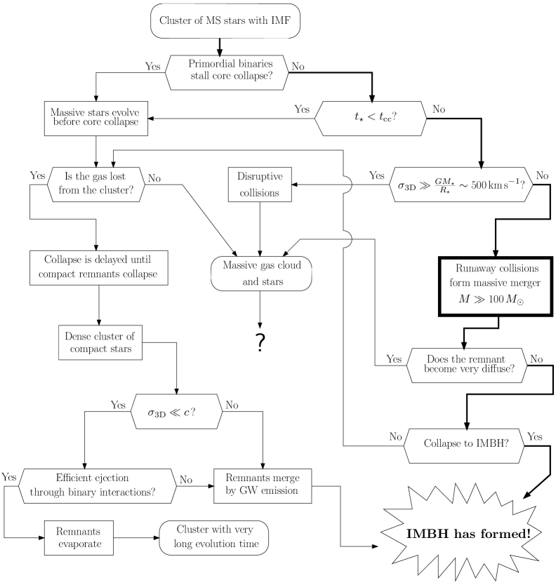
Figure 1.— Various possible scenarios for the early dynamical evolution of a dense star cluster with a realistic IMF. The path for the formation of an IMBH through core collapse and runaway collisions (studied in this paper) is indicated by a thicker line. An alternative scenario involves successive mergers of stellar-mass BH binaries driven by a combination of dynamical interactions and gravitational radiation (left side of the diagram). For a runaway to occur, the core collapse time $t_{\rm cc}$ must be smaller than the stellar lifetime $t_{*}$ of the most massive stars in the cluster. High-velocity disruptive collisions, the formation of a very extended and diffuse merger remnant, or the accumulation in the cluster of gas released by stellar winds and supernova explosions could lead to the formation of a complex system containing stars embedded in a dense gas clouds. The final fate of such a system is highly uncertain.

When they are born, star clusters are expected to contain many young stars with a wide range of masses, from $\sim 0.1M_{\odot}$ to $\sim 100M_{\odot}$, distributed according to a Salpeter-like initial mass function (IMF) (Clarke, 2003). Inspired by an early version from Rees (1984) for the formation of supermassive BH, we show in Figure 1 a diagram illustrating the two main scenarios leading to the formation of an IMBH at the center of a dense star cluster. The early stages of dynamical evolution are dominated by the stars in the upper part of the mass spectrum. Through dynamical friction, these heavy stars tend to concentrate toward the center and drive the system to core collapse. Successive collisions and mergers of the massive stars during core collapse can then lead to a runaway process and the rapid formation of a very massive object containing the entire mass of the collapsing cluster core. Although the fate of such a massive merger remnant is rather uncertain, direct “monolithic” collapse to a BH with no or little mass loss is a likely outcome, at least for sufficiently small metallicities (Heger et al., 2002). An essential condition for this runaway to occur is that the core collapse must occur before the most massive stars born in the cluster end their lives in supernova explosions (Portegies Zwart & McMillan, 2002; Rasio et al., 2003).

The accumulation at the center of a galaxy of many IMBH produced through this runaway process in nearby young star clusters (like the Arches and Quintuplet clusters in our Galaxy) provides an interesting new way of building up the mass of a central supermassive BH (Portegies Zwart & McMillan, 2002). It is possible that this process of accumulation is still ongoing in our own Galaxy (Hansen & Milosavljević, 2003). These ideas have potentially important implications for the study of supermassive BH by the Laser Interferometer Space Antenna (LISA), since the inspiral of IMBH into a supermassive BH provides the best source of low-frequency gravitational waves for direct study of strong field gravity (Cutler & Thorne, 2002).

In the alternative scenario where massive stars evolve and produce supernovae before the cluster goes into core collapse, a subsystem of stellar-mass BH will be formed (Figure 1). As demonstrated in Section 4.5, the mass loss from supernovae provides significant indirect heating of the cluster core, delaying the onset of core collapse until much later, after the stellar remnants undergo mass segregation. The final fate of a cluster with a component of stellar-mass BH remains highly uncertain. This is because realistic dynamical simulations for such clusters (containing a large number of black holes and ordinary stars with a realistic mass spectrum) have yet to be performed. For old and relatively small systems (such as Galactic globular clusters), complete evaporation is likely (with all the stellar-mass BH ejected from the cluster through 3-body and 4-body interactions in the dense core). This is expected theoretically on the basis of simple qualitative arguments (Kulkarni et al., 1993; Sigurdsson & Hernquist, 1993) and has been demonstrated recently by direct $N$-body simulations for very small systems containing only $\sim 10$ BH (Portegies Zwart & McMillan, 2000). However, for larger systems (more massive globular clusters or proto-galactic nuclei), contraction of the cluster to a highly relativistic state could again lead to successive mergers (driven by gravitational radiation) and the formation of a single massive BH (Quinlan & Shapiro, 1989; Lee, 1995, 2001). Moreover, it has been recently suggested that, if stellar-mass BH are formed with a broad mass spectrum (a likely outcome for stars of very low metallicity; see Heger et al. 2003), the most massive BH could resist ejection, even in a system with low escape velocity such as a globular cluster. These more massive BH could then grow by repeatedly forming binaries (through exchange interactions) with other BH and merging with their companions (Miller & Hamilton, 2002). However, as most interactions will probably result in the ejection of one of the lighter BH, it is unclear whether any object could grow substantially through this mechanism before running out of companions to merge with.

1.2. Core Collapse and the Spitzer Instability

The physics of gravothermal contraction and core collapse is by now very well understood for single-component systems (containing all equal-mass stars). In particular, the dynamical evolution of an isolated, single-component Plummer sphere to core collapse has been studied extensively and has become a testbed for all numerical codes used to compute the evolution of dense star clusters (Aarseth et al., 1974; Giersz & Spurzem, 1994). This evolution can be visualized easily using Lagrange radii, enclosing a fixed fraction of the total mass of the system see, e.g., Fig. 3 of Joshi et al., 2000 and Fig. 5 of Freitag & Benz, 2001. As the system evolves, the inner Lagrange radii contract while the outer ones expand. This so-called gravothermal contraction results from the negative heat capacity that is a common property of all gravitationally bound systems (Elson et al., 1987). In the absence of an energy source in the cluster core, and in the point-mass limit (i.e., neglecting physical collisions between stars), the contraction of the cluster core becomes self-similar and continues indefinitely. This phenomenon is known as core collapse and its universality is very well established (see, e.g., Freitag & Benz, 2001, Table 1 and references therein).

Figure 2.— Evolution of single-component and Salpeter-IMF Plummer models to core collapse. Lagrange radii enclosing a constant mass fraction, indicated on the left, are shown as a function of time. The radii are in units of the initial half-mass radius of the cluster and time is in units of the initial half-mass relaxation time. The solid lines are from our Monte Carlo simulation of a Plummer model containing $1.25\times 10^{6}$ stars with a Salpeter IMF (within $m_{\rm min}=0.2\,M_{\odot}$ and $m_{\rm max}=120\,M_{\odot}$). The dotted lines show the result of a gaseous model simulation of the same cluster, with 50 discrete mass components approximating a Salpeter IMF (within the same mass limits). See Sec. 2 for more discussions of the various methods. For comparison, the dashed lines show the evolution of a single-component Plummer Model (computed with our Monte Carlo code). Note our key result: the core collapse time is more than two orders of magnitude shorter for a cluster with a realistic IMF.

When the system contains stars with a variety of masses, the evolution to core collapse is accelerated. This has been demonstrated by the earliest $N$-body and Monte Carlo simulations (Aarseth, 1966; Hénon, 1971a; Wielen, 1975). To illustrate this behavior, and as a preview of the results presented later in Sec. 4, we show in Figure 2 the evolution of a cluster described initially by a simple Plummer model containing $1.25\times 10^{6}$ stars with a broad Salpeter IMF between $m_{\rm min}=0.2\,M_{\odot}$ and $m_{\rm max}=120\,M_{\odot}$. Core collapse occurs after $\lesssim 0.1\,t_{\rm rh}(0)$, where $t_{\rm rh}(0)$ is the initial half-mass relaxation time (see eq. (6) below). In sharp contrast, core collapse in a single-component Plummer model occurs after $\gtrsim 10\,t_{\rm rh}(0)$ (a well-known result). Thus the presence of a broad IMF can dramatically accelerate the evolution of the cluster to core collapse.

This acceleration of the evolution to core collapse is due to the changing nature of energy transfer in the presence of a wide mass spectrum. Relaxation processes tend to establish energy equipartition (see, e.g., Binney & Tremaine, 1987, Sec. 8.4). In a cluster where the masses of the stars are nearly equal, this can be (very nearly) achieved. The core collapse is then a result of energy transfer from the inner to the outer parts of the cluster, leading to gravothermal contraction (Lynden-Bell & Wood, 1968; Larson, 1970). A large difference between the masses of the stars allows a more efficient mechanism for energy transfer. In this case, energy equipartition would tend to bring the heavier stars to lower speeds. However, as a result, the heavier stars sink to the center, where they tend to gain kinetic energy, while the lighter stars move to the outer halo. This process is called “mass segregation.” As the mass segregation proceeds, the core contracts and gets denser, leading to a shorter relaxation time, which in turn increases the rate of energy transfer from heavier to lighter stars. In typical cases this evolution eventually makes the heavier stars evolve away from equipartition (Spitzer, 1969).

The fundamental inability of the heavier stars to establish energy equipartition with the lighter stars in a system with a continuous mass spectrum is similar to the Spitzer “mass-segregation instability” in two-component clusters. Spitzer (1969), using analytic methods and a number of simplifying assumptions, determined a simple criterion for a two-component system to achieve energy equipartition in equilibrium. If the mass of the lighter (heavier) stars is $m_{1}$ ($m_{2}$) and the total mass in the light (heavy) component is $M_{1}$ ($M_{2}$), then Spitzer’s criterion can be written

$$S\equiv\left(\frac{M_{2}}{M_{1}}\right)\left(\frac{m_{2}}{m_{1}}\right)^{3/2}<0.16.$$ (1)

Watters et al. (2000), using numerical simulations, obtained a more accurate empirical condition,

$$\Lambda\equiv\left(\frac{M_{2}}{M_{1}}\right)\left(\frac{m_{2}}{m_{1}}\right)^{2.4}<0.32.$$ (2)

When this stability criterion is not satisfied, energy equipartition cannot be established between heavy and light stars. Spitzer (1969) noted that the equilibrium would not be achieved for realistic mass spectra, because there is always sufficient mass in high-mass stars that, through mass segregation, they can form a subsystem (near the center of the cluster) that decouples dynamically from the lower-mass stars. This was later supported by more detailed theoretical studies (Saslaw & De Young, 1971; Vishniac, 1978; Inagaki & Saslaw, 1985).

Here we carry out a simple calculation to show that a typical system, with a Salpeter IMF (see Sec. 3.2) extending from $0.2\,M_{\odot}$ to $120\,M_{\odot}$, when viewed as a two-component cluster of “light stars” and “heavy stars,” does not satisfy any of the simple stability criteria. Let us separate the stars into these two components according to some arbitrary boundary: we group all stars lighter than $m_{\rm b}$ in the first component, and all stars heavier than $m_{\rm b}$ in the second component. We use $m_{1}$ and $M_{1}$ to denote the values of the average and total mass in the first component, and $m_{2}$ and $M_{2}$ similarly for the second component. We obtain, with $m_{\rm b}$ in solar mass,

$$\frac{M_{1}}{M_{2}} =\frac{0.2^{-0.35}-m_{\rm b}^{-0.35}}{m_{\rm b}^{-0.35}-120^{-0.35}},{\rm~{}~{}~{}~{}~{}~{}~{}and}$$ (3)

$$\frac{m_{1}}{m_{2}} =\frac{M_{1}}{M_{2}}\cdot\frac{N_{2}}{N_{1}}=\frac{0.2^{-0.35}-m_{\rm b}^{-0.35}}{m_{\rm b}^{-0.35}-120^{-0.35}}\cdot\frac{m_{\rm b}^{-1.35}-120^{-1.35}}{0.2^{-1.35}-m_{\rm b}^{-1.35}}.$$ (4)

When these values are used in equations (1) and (2) we see (Figure 3) that the stability criteria are almost never satisfied for any value of $m_{\rm b}$, except when it is extremely close to the maximum mass (as expected, since the model reduces artificially to a single-component system in this limit, with all stars having the average mass).

Vishniac (1978), devised a criterion genuinely adapted to clusters with a continuous mass spectrum, under the ad-hoc assumption that the shape of the density distribution does not depend on the stellar mass. He derives the following necessary condition for stability:

$$\beta\left(\frac{m_{\rm b}}{m_{1}}\right)^{3/2}\frac{M_{2}}{M_{1}+M_{2}}<1,\ \ \mbox{with}\ \ \beta\simeq 0.5,$$ (5)

for all $m_{\rm b}$ (his eq. 17). Figure 3 shows that this condition cannot be satisfied either. These results suggest that for any Salpeter-like IMF, one can always find a collection of stars that have large enough average and total mass that they will dynamically decouple from the lighter stars in the cluster. Once these decouple they form a subsystem with a much shorter relaxation time and consequently evolve to core collapse very rapidly.

Figure 3.— Various criteria for the realization of equipartition in a cluster with a Salpeter IMF. According to these, energy equipartition in dynamical equilibrium can only be achieved if the corresponding curve lies entirely under the dotted horizontal line. Conditions by Spitzer and Watters et al. were devised for two-component models, so we divide the mass function into stars lighter and heavier than some arbitrary boundary value $m_{\rm b}$ and we evaluate the stability conditions for any value of $m_{\rm b}$. Vishniac’s analysis is genuinely adapted to a continuous mass function. He derives a necessary condition for stable equipartition that must be obeyed for any stellar mass $m_{\rm b}$ in the range covered by the mass spectrum. See text for details.

The half-mass relaxation time (relaxation time at the half-mass radius $r_{h}$) for a cluster of $N$ stars is given by (Spitzer, 1987, eq. 2.63):

$$t_{\rm rh}(0)=\frac{0.138N}{\ln(\gamma_{\rm c}N)}\left(\frac{r_{\rm h}^{3}}{GM}\right)^{1/2}\propto\frac{N/\ln(\gamma_{\rm c}N)}{\rho^{1/2}}\>,$$ (6)

where $\rho$ is the mass density and $\gamma_{\rm c}\sim 0.01$ in the Coulomb logarithm. Let us assume that a collapsing subsystem is formed by stars that constitute 1% of the total mass, and that all of them come from the uppermost part of the mass spectrum. For a Salpeter IMF with $m_{\rm min}=0.2\,M_{\odot}$ and $m_{\rm max}=120\,M_{\odot}$, the number of stars in this subsystem is then $N_{\rm sub}\lesssim 10^{-4}N$. At the time of dynamical decoupling the central density of the subsystem must be comparable to the central density of the overall cluster. Therefore we conclude that the relaxation time is around three orders of magnitude smaller for the collapsing subsystem of heavy stars at the onset of instability. So, essentially, the heavy stars will go into core collapse as soon as they start dominating the mass density near the center.

If the cluster starts its evolution with heavy stars distributed throughout, the timescale for core collapse will be determined by their mass segregation timescale. The process of mass segregation for the heaviest stars in the cluster is driven by dynamical friction (Binney & Tremaine, 1987, Section 7.1). The timescale for mass segregation and the onset of core collapse therefore depends primarily on the mass ratio between the dominant heavy stars and the lighter background stars (Spitzer, 1969; Chernoff & Weinberg, 1990). For simple dynamical friction in an effective two-component model, one would then expect the core collapse time to be comparable to $t_{\rm DF}\equiv(m_{\rm b}/\left<m\right>)\,t_{\rm rh}$. Here $m_{\rm b}$ ($\ll m_{\rm max}$, the upper mass limit of the IMF) should be the mass above which the IMF contains a large enough number of massive stars to define a “collapsing subsystem.” If this number is $\sim 10^{3}$ and the total number of stars $N\sim 10^{6}$ we get $m_{\rm b}\simeq 20\,M_{\odot}$ for our standard Salpeter IMF and this simple analysis would then predict the correct order of magnitude for the core collapse time ($t_{\rm cc}/t_{\rm rh}(0)\sim 0.1$; see Figure 2). Note, however, that this simple dynamical friction picture corresponds to one or a few massive objects traveling through a uniform background of much lighter particles, a description that provides, at best, only a rough approximation of the real situation under consideration here (see Appendix).

1.3. Goals of this Study

In this paper, the first of a series, we consider a wide variety of initial cluster models and we investigate the evolution of all systems until the onset of core collapse. Results from numerical simulations that include stellar collisions and track the growth of a massive object through successive mergers of massive stars during core collapse will be presented in a subsequent paper. This work is in progress and preliminary results have already been reported elsewhere (Rasio et al., 2003). Here we determine how the core collapse time is related to various initial parameters including the IMF (Sec. 3.2 and 4.2) and the central concentration and tidal radius of the cluster (Sec. 3.1 and 4.3), and we also include the possibility of initial mass segregation (Sec. 3.3 and 4.4). We then make a comparison with the stellar evolution time and derive limits on cluster initial conditions to allow the development of runaway collisions and the possible subsequent formation of a central massive BH (Sec. 5). We also derive from our calculations an estimate of the total mass of the stars that participate in the runaway collisions, which provides an upper limit to the final BH mass.

We do not include stellar evolution in our calculations since our aim here is to investigate dynamical processes taking place before even the most massive main-sequence stars in the cluster have evolved. We do, however, study the effects of mass loss from stellar winds and their dependence on metallicity (Sec. 4.5). In a subsequent paper (Gürkan & Rasio, 2003), we will study the evolution of “post-collapse” star clusters in which a central IMBH is assumed to have formed early on (through the runaway collision process). In particular, we will study the possibility that mass loss from the stellar evolution of the remaining massive stars (those that have escaped the central collapse and runaway) could disrupt the cluster (cf. Joshi et al., 2001), thereby producing a “naked” IMBH. This is motivated by observations of ultraluminous X-ray sources in regions of active star formation (e.g., in merging galaxies) containing many young star clusters, but with the X-ray sources found predominantly outside of those clusters (Zezas & Fabbiano, 2002).

An important factor that could affect significantly the dynamics of core collapse in young star clusters is the presence of primordial binaries (Fregeau et al., 2003a) or the dynamical formation of binaries through three-body interactions (Hut, 1985; Giersz, 1998). As pointed out by Inagaki (1985), the formation rate of hard three-body binaries would be accelerated in clusters with a mass spectrum (Heggie, 1975). In this first paper we do not take into account the presence of binaries in the cluster. This is justified because we do not expect binaries to play an important role until after the onset of core collapse, when the central density increases suddenly. However, collisions should become dominant immediately after the onset of core collapse. Our expectation, based on several previous theoretical studies of physical collisions during interactions of hard primordial binaries and for three-body binary formation, is that the presence of binaries in the core will in fact increase collision rates, thereby helping to trigger the runaway (Chernoff & Huang, 1996; Bacon et al., 1996; Fregeau et al., 2003b). This is also supported by the results of direct $N$-body simulations showing that, in smaller systems containing $N\gtrsim 10^{4}$ single stars, collisions indeed occur predominantly through the interactions of three-body binaries formed at core collapse (Portegies Zwart & McMillan, 2002).

2. Numerical Methods and Summary of Previous Work

Numerical methods for investigating the dynamical evolution of star clusters include direct $N$-body integration, solutions of the Fokker-Planck equation by direct (finite-difference) or Monte Carlo methods, and gaseous models (for a review, see Heggie & Hut, 2003). Here we refer to direct $N$-body integrations simply as “$N$-body simulations,” direct integrations of the Fokker-Planck equation as “Fokker-Planck (FP) simulations,” and Fokker-Planck simulations based on Monte Carlo techniques as “Monte Carlo (MC) simulations.” Note, however, that our MC simulations, in which the cluster is modeled on a star-by-star basis, are in fact another type of “$N$-body simulations.” Each approach offers different advantages and disadvantages for understanding core collapse and massive black hole formation in star clusters with a realistic mass spectrum.

2.1. Summary of Previous Numerical Work

Portegies Zwart & McMillan (2002) carried out $N$-body simulations starting from a variety of initial conditions for clusters containing up to $\sim 6\times 10^{4}$ stars. They found that runaway collisions driven by the most massive stars can happen in sufficiently dense clusters. Their results apply directly to small star clusters containing $\sim 10^{4}-10^{5}$ stars. However, in such a small cluster, any realistic IMF typically contains only a very small number of massive stars. For example, a Salpeter IMF with minimum mass $m_{\rm min}=0.2\,M_{\odot}$ and maximum mass $m_{\rm max}=120\,M_{\odot}$ contains a fraction $\sim 3\times 10^{-4}$ of its stars above $60\,M_{\odot}$. The dynamical role played by massive stars can therefore depend strongly on the total number of stars in the cluster. In addition, in small systems, the dynamical evolution might be dominated by the random behavior or the initial conditions of just a few very massive stars. Consequently, to investigate runaway collisions in larger systems such as super star clusters or proto-galactic nuclei, realistically large numbers of stars must be used in numerical simulations. The computational time required for direct integration of an $N$-body system over one crossing time $t_{\rm dyn}$ scales as $N^{2}$ ($N^{1.25}$ on parallel machines, if one can adjust the number of CPUs to $N$ optimally; see Spurzem & Baumgardt 2003). Since the relaxation time is $\sim(N/\ln N)\,t_{\rm dyn}$ (see Sec. 1.2), the scaling of the total CPU time of $N$-body simulations is nearly as steep as $N^{3}$. Currently, using a state-of-the-art GRAPE-6 board to accelerate the computations (Makino, 2001, 2002), the evolution of a cluster containing $10^{5}$ stars with $m_{\rm max}/m_{\rm min}=1000$ and no primordial binaries can be integrated up to core collapse in about one day (H. Baumgardt, private communication). However, including primordial binaries or increasing the number of stars would still lead to prohibitively long computation times, especially for a parameter study where a large number of integrations are required.

A wide mass spectrum also leads to increased computation times for FP simulations and gaseous models. In these methods, a continuous mass spectrum is approximated by discrete mass bins. In the gaseous model, the most time-consuming operation of the algorithm is the inversion of large matrix whose dimension is proportional to the number of equations, itself proportional to $N_{\rm comp}$. Hence the computing time increases like $T_{\rm CPU}\propto N_{\rm comp}^{3}$. For FP codes, there is one diffusion term coupling each component to all others, leading to $T_{\rm CPU}\propto N_{\rm comp}^{2}$. These steep scalings limit $N_{\rm comp}$ to at most $\sim 20$ to avoid computation times longer than a few days.

Even with a small number of mass bins, FP simulations have yielded important qualitative results. Inagaki and collaborators investigated two- and multi-component systems (Inagaki & Wiyanto, 1984; Inagaki, 1985; Inagaki & Saslaw, 1985). They found that the energy transfer within the core is an important process for determining the onset of core collapse. FP simulations by Inagaki (1985) and Chernoff & Weinberg (1990) show that a mass function with $m_{\rm max}/m_{\rm min}\simeq 10-15$ needs to be discretized into about 15 components or more to obtain an accurate value of the core collapse time. A coarser discretization leads to an artificially slow evolution. Chernoff & Weinberg (1990) successfully tracked the energy transfer between different components and demonstrated the importance of this process. Quinlan (1996) used FP simulations to follow the evolution of single- and two-component systems. He used a unique setting for his two-component clusters, with each component having a different initial spatial distribution. His aim was to study the interaction of galactic nucleus containing mainly dark (compact) objects with the bulge of the galaxy. In one model he considered a structure with “inverse initial mass segregation,” where the central nucleus is made of objects much lighter than the normal stars composing the bulge. He showed that this situation also leads to highly accelerated evolution as the more massive stars get trapped by the nucleus through dynamical friction and undergo rapid core collapse. Takahashi (1997) also investigated the evolution of clusters with a mass spectrum using FP simulations. His simulations were two-dimensional (in phase space) and therefore he was able to study the development of velocity anisotropy.

Gaseous models have the advantage of being very fast (for $N_{\rm comp}\lesssim 20$) but they include the greatest number of simplifying assumptions and so require independent checking. The good agreement shown with our MC simulation for a Plummer model with Salpeter IMF in Figure 2 is encouraging. Note, however, that the gaseous model calculation shown in Figure 2 used 50 mass components. This number of components is exceptionally high, leading to a total computation time in excess of three weeks, much longer than most MC runs. It was chosen to be able to follow core collapse to a very advanced stage, until the most massive component dominates the collapsing core. We note that the evolution of the gaseous model to core collapse is faster by some 30 % and exhibits a more gradual contraction of the inner region. The reasons for these small discrepancies will be investigated in future work, where additional comparisons between Monte Carlo and gaseous model calculations will also be presented (Freitag et al., 2003a). For the time being, suffice it to mention that for multi-mass clusters, there are basically two adjustable (dimensionless) parameters in the gaseous model, one setting the effective thermal conductivity and the other the timescale for energy exchange between components ($\lambda$ and $\lambda_{\rm eq}$, see Louis & Spurzem 1991; Giersz & Spurzem 1994; Spurzem & Takahashi 1995). For the model plotted in Figure 2, we used the standard values of these parameters ($\lambda=0.4977$ and $\lambda_{\rm eq}=1$) which were established for clusters with a different structure and mass spectrum and some adjustment (preferentially through comparisons with $N$-body runs) may be required.

A direct comparison between FP and gaseous models was also carried out by Spurzem & Takahashi (1995), for two-component clusters, and also resulted in good agreement. Recently, a hybrid code has been developed by Giersz & Spurzem (2003), combining a gaseous model with MC techniques. In this approach the single stars are represented by the gaseous model, while primordial binaries are followed with a Monte Carlo treatment. A similar hybrid treatment could be applied to the problem we are studying here, but with massive (single and binary) stars included in the Monte Carlo component, and lower-mass stars represented by a gaseous model.

2.2. The Monte Carlo Code

The solution of the Fokker-Planck equation with an orbit-averaged Monte Carlo method is an ideal compromise for the problem at hand. It can handle a suitably large number of stars and a wide mass spectrum can be implemented with very little additional difficulty. Most importantly, as in direct $N$-body integrations, MC simulations can implement a star-by-star description of the cluster. This allows the inclusion of many important processes such as collisions, binary interactions (including primordial binaries), stellar evolution (and the accompanying mass loss), as well as the effects of a massive central object with relative ease and much higher realism compared to direct FP simulations or gaseous models. We will incorporate the effects of all these additional processes on cluster evolution in the subsequent papers of this series.

The MC code we have used to obtain the main results of this paper is described in detail by Joshi et al. (2000). It is based on the ideas of Hénon (1971a, b, 1973) and in many respects it is very similar to MC codes developed by Stodółkiewicz (1982, 1986), Giersz (1998, 2001), and Freitag & Benz (2001). In the rest of this section, we give a brief summary of the numerical method.

The main simplifying assumption is the Fokker-Planck approximation, in which relaxation processes are assumed to be dominated by small distant encounters rather than strong encounters with large deflections (Spitzer, 1987; Binney & Tremaine, 1987). The dynamical evolution can then be treated as a diffusion process in phase space. Following the individual interactions between the stars, as in direct $N$-body simulations, is computationally expensive. However, the average cumulative effect on a star in a given amount of time can be characterized by diffusion coefficients in phase space. To compute the relaxation, the timestep for the numerical evolution has to be chosen smaller than the relaxation time. Since the relaxation time is normally shortest at the center, we choose our timestep to be a fraction of the central relaxation time. This ensures that the relaxation is followed accurately throughout the cluster.

Another important simplification in the MC method is the assumption of spherical symmetry. The position of the particles is represented by a single radial coordinate, $r$, and the velocity is represented by radial, $v_{r}$, and tangential, $v_{t}$, components. The specific angular momentum, $A$, and the specific energy, $E$, of a star with index $i$, are given by:

$$A_{i}=v_{t,i}\,{r_{i}}\>,\quad E_{i}=U(r_{i})+\frac{1}{2}(v_{r,i}^{2}+v_{t,i}^{2}),$$ (7)

where $U(r)$ is the gravitational potential at a given point. The assumption of spherical symmetry implies that the potential at all points can be computed in a time proportional to the number of particles $N$, rather than $N^{2}$.

In Hénon’s algorithm, the evolution is simulated by reproducing the effect of the cluster on each star by a single effective encounter in each timestep. At every iteration the two integrals of the motion $A_{i}$ and $E_{i}$ characterizing the orbit of each star are perturbed in a way that is consistent with the value of the diffusion coefficients (Hénon, 1973). To conserve energy, this perturbation is realized by a single effective scattering between two neighboring stars. The square of the scattering angle, $\beta$, is proportional to the timestep chosen. We choose our timestep such that $\sin^{2}(\beta/2)\lesssim 0.05$ at the center of the cluster. Choosing too large a timestep will lead to a saturation effect and the relaxation will proceed artificially slowly. Using too small a timestep, on the other hand, not only increases the computation time, but also can lead to spurious relaxation (see the Appendix for a discussion of spurious relaxation effects).

After the perturbation of $A_{i}$ and $E_{i}$, the stars are placed at random positions between their apocenters and pericenters using a probability distribution that is proportional to the time spent at a given location on their new orbit. For a star with index $i$, the apocenter and pericenter distances are calculated by finding the roots of

$$2E_{i}-2U(r)-\frac{A_{i}^{2}}{r^{2}}=0.$$ (8)

This random placement is justified by the assumption of dynamical equilibrium, i.e., the evolution of the system does not take place on the crossing (or dynamical) timescale, but rather on the relaxation timescale. The only important point about assigning a specific position to a particle on its orbit is that its contribution to density, potential, interaction rates, etc., has to be estimated correctly. After all stars have been placed at their new positions, the potential is recalculated and the whole cycle of perturbation is repeated.

This method can be modified so that the timestep is a fraction of the local relaxation time (Hénon, 1973; Freitag & Benz, 2001). Stodółkiewicz (1982, 1986) and Giersz (1998, 2001) divided the system into zones resulting in an approach intermediate between a fixed and smoothly varying timestep. Dividing the system into radial zones also allows the MC method to be parallelized efficiently for use on multi-processor machines (Joshi et al., 2000). Another possible modification uses a scaling of the units such that each particle in the simulation can represent an entire spherical shell of many identical stars rather than a single star (Hénon, 1971a; Freitag & Benz, 2001, 2002). It should also be noted that, although the effects of strong encounters between stars on relaxation are assumed to be negligible compared to weak, more distant encounters, they can be incorporated by estimating their rate of occurrence in a way similar to physical collisions (Freitag & Benz, 2002) or interactions with binary stars (Fregeau et al., 2003a).

Our MC code has been used previously to study many fundamental dynamical processes such as the Spitzer instability (Watters et al., 2000) and mass segregation (Fregeau et al., 2002) for simple two-component systems, as well as the evolution of systems with a continuous but fairly narrow mass spectrum of evolving stars (Joshi et al., 2001). A difficulty introduced by a broad continuous IMF (with a large $m_{\rm max}/m_{\rm min}$ ratio) is the necessity of adjusting the timestep to treat correctly encounters between stars of very different masses. When pairs of stars are selected to undergo an effective hyperbolic encounter as described above, one has to make sure that the deflection angle remains small for both stars. In situations where the mass ratio of the pair can be extreme, one has to decrease the timestep accordingly (Stodółkiewicz, 1982). In practice, for the simulations described here, we find that the timestep has to be reduced by a factor of up to $\sim 500$ compared to what would be appropriate for a cluster of equal-mass stars. We discuss further the applicability of orbit-averaged MC methods to systems with a continuous mass spectrum and large $m_{\rm max}/m_{\rm min}$ ratio in the Appendix.

3. Initial Conditions and Units

The characteristics of core collapse and the subsequent runaway collisions depend on the initial conditions for the cluster. These initial conditions include the total number of stars, the IMF, the initial spatial distribution of the stars (density profile and, possibly, initial mass segregation), and the position of the cluster in the galaxy, which determines the tidal boundary. As we shall see, the most important initial parameters are the slope of the IMF, the maximum stellar mass, and the initial degree of central concentration of the cluster density profile. We have used a wide variety of initial conditions, both to test the robustness of our findings and to establish the dependence of our results on these parameters. As a typical reference model we use an isolated Plummer sphere with a Salpeter IMF and stellar masses ranging from $m_{\rm min}=0.2\,M_{\odot}$ to $m_{\rm max}=120\,M_{\odot}$. We then explore variations on this model by changing the initial cluster structure, the IMF or the number of stars.

3.1. Density Profile

We have examined three families of models: Plummer and King models (Binney & Tremaine, 1987, Sections 2.2 and 4.4), which have a core-halo structure, and $\gamma$-models (Dehnen, 1993; Tremaine et al., 1994), which have a cusp near the center. All these models have a characteristic radius given by

$$a_{\rm P} =(2^{2/3}-1)^{1/2}r_{\rm h}\simeq 0.766\,r_{\rm h},$$ (9)

$$a_{\rm K} =\sqrt{\frac{9\sigma^{2}}{4\pi\,G\,\rho_{0}}},$$ (10)

$$a_{\gamma} =(2^{1/(3-\gamma)}-1)r_{\rm h},$$ (11)

for Plummer, King, and $\gamma$-models respectively. In these formulae, $r_{\rm h}$ is the half-mass radius, $\rho_{0}$ is the central density, and $\sigma$ is a King model parameter. We show the density profiles corresponding to these various models in Figure 4. Here $W_{0}$ is the dimensionless central potential, related to the concentration parameter (Binney & Tremaine, 1987, Fig. 4-10). Other useful quantities characterizing the various density profiles are given in Table 1. The initial model used for each of our MC simulations is listed in the second column of Table 2. A general procedure for producing these models is given by Freitag & Benz (2002); a less general but simpler procedure for the Plummer model is given by Aarseth et al. (1974).

Table 1Properties of clusters

Cluster	$\rho_{0}$	$\sigma_{0}$	$a$	$r_{\rm t}$	$r_{\rm h}$	$r_{\rm c}$	$M_{\rm c}$	$t_{\rm rh}$	$t_{\rm rc}$
Plummer	1.167	0.532	0.589	$\infty$	0.769	0.417	0.192	0.093	0.0437
King $W_{0}=1$	0.454	0.534	1.517	2.568	0.858	0.670	0.321	0.110	0.1134
2	0.530	0.526	1.003	2.800	0.849	0.612	0.281	0.108	0.0930
3	0.652	0.518	0.749	3.134	0.839	0.543	0.238	0.106	0.0722
4	0.860	0.510	0.576	3.625	0.827	0.465	0.195	0.104	0.0523
5	1.252	0.504	0.438	4.362	0.814	0.382	0.1546	0.101	0.0348
6	2.112	0.503	0.320	5.471	0.804	0.293	0.1171	0.100	0.0205
7	4.526	0.511	0.2146	6.987	0.812	0.2032	0.0830	0.101	0.00997
8	13.742	0.530	0.1253	8.344	0.872	0.1211	0.0531	0.112	0.00368
9	55.671	0.558	0.0649	8.374	0.980	0.0633	0.0307	0.134	0.00106
$\gamma=1.0$	$\infty$	0	$1/3$	$\infty$	0.805	0	0	0.100	0
$1.5$	$\infty$	0	$1/2$	$\infty$	0.851	0	0	0.108	0

Note. — Definitions of quantities listed in this table: $\rho_{0}$ is the central mass density; $\sigma_{0}$ is the central one-dimensional velocity dispersion; $a$ is the characteristic radius (see Eqs. 9–11); $r_{\rm t}$ is the tidal radius; $r_{\rm h}$ is the half-mass radius; $r_{\rm c}\simeq\left[9\sigma_{0}^{2}/(4\pi G\rho_{0})\right]^{1/2}$ is the core radius; $M_{\rm c}$ is the mass enclosed by $r_{\rm c}$; $t_{\rm rh}$ is the half-mass relaxation time (eq. 6); and $t_{\rm rc}$ is the central relaxation time (eq. 18). All quantities are given in $N$-body units, except that $t_{\rm rh}$ and $t_{\rm rc}$ are given in “Fokker-Planck units” (see Section 3.4).

Figure 4.— Density profiles for various initial models used in our simulations. The Plummer model is shown by a solid line, $\gamma$-models corresponding to $\gamma=1,\,1.5$ and 2 are shown by dotted lines, and King models with $W_{0}=3,\,6,\,9$ and 12 are shown by dashed lines. The radius is in units of the characteristic length scale parameter of each model and the density profiles are normalized to unity at that radius. King models with lower $W_{0}$ values have steeper profiles outside $r=a_{\rm K}$, while $\gamma$-models with higher $\gamma$ values have higher $\rho/\rho(a)$ near the center.

3.2. Initial Mass Function

Since we expect the conditions leading to core collapse to depend sensitively on the IMF, we have carried out simulations with a wide range of IMF parameters. However, it is generally established that, at least for the high-mass end of the spectrum, a universal IMF very close to the simple Salpeter-like power-law is obeyed. This is indicated both by observations and by theoretical calculations (Kroupa, 2002; Clarke, 2003, and references therein).

In our simulations we assign the masses of individual stars using a sampling procedure. We first choose a random number, $X$, from a uniform distribution between 0 and 1. For a simple power-law IMF with $dN\propto m^{-\alpha}\,dm$ between $m_{\rm min}$ and $m_{\rm max}$ we calculate the corresponding mass using

$$m(X)=m_{\rm min}\left(1+X\left[\left(\frac{m_{\rm max}}{m_{\rm min}}\right)^{1-\alpha}-1\right]\right)^{1/(1-\alpha)},$$ (12)

where the value $\alpha=2.35$ would correspond to a Salpeter IMF.

In addition to simple power laws, for two models we have used the Miller-Scalo (1979) and Kroupa (Kroupa et al., 1993) IMFs, which are steeper at the high-mass end of the spectrum and shallower at the low-mass end. Both of these IMFs can be represented by broken power laws. For the Miller-Scalo IMF,

$$\frac{dN}{dm}\propto\begin{cases}m^{-1.4}\;&0.1\leq m\leq 1.0\\ m^{-2.5}\;&1.0\leq m\leq 10.0\\ m^{-3.3}\;&10.0\leq m\end{cases},$$ (13)

and for the Kroupa IMF,

$$\frac{dN}{dm}\propto\begin{cases}m^{-1.3}\;&0.08\leq m\leq 0.5\\ m^{-2.2}\;&0.5\leq m\leq 1.0\\ m^{-2.7}\;&1.0\leq m\end{cases},$$ (14)

where all numerical values are in solar mass.

However, for the sake of computational convenience, we prefer to implement a somewhat different parametrization of these distributions. To generate the mass spectra corresponding to these IMFs we use the functions (Eggleton et al., 1989; Kroupa et al., 1993)

$$m(X)=\frac{0.19X}{(1-X)^{0.75}+0.032(1-X)^{0.25}}$$ (15)

and

$$m(X)=0.08+\frac{0.19X^{1.55}+0.05X^{0.6}}{(1-X)^{0.58}},$$ (16)

for the Miller-Scalo and Kroupa mass functions, respectively. In both cases if $m(X)<m_{\rm min}$ or $m(X)>m_{\rm max}$ the result is discarded and a new random number is generated. The values in equation (16) correspond to the choice of $\alpha_{1}=1.3$ in Table 10 of Kroupa et al. (1993).

In most of our simulations we have used $N=1.25\times 10^{6}$ stars. For all mass functions, this implies the presence of many massive stars, allowing us to resolve fully the higher end of the mass spectrum. For example, for $m_{\rm min}=0.2\,M_{\odot}$ and $m_{\rm max}=120\,M_{\odot}$, with $N=1.25\times 10^{6}$, we have $\gtrsim 60$ stars with $m>100\,M_{\odot}$ for a Salpeter IMF. The results from our simulations are therefore not much affected by random fluctuations in a small number of very massive stars. Note, however, that in much smaller systems, containing perhaps only $\sim 10^{4}$ stars (as in the Arches and Quintuplet clusters near our Galactic center), these small number effects and random fluctuations may indeed play a dominant role in determining the dynamical fate of the few most massive stars in the system.

3.3. Initial Mass Segregation

Initial mass segregation in star clusters (i.e., the tendency for more massive stars to be formed preferentially near the cluster center) is expected to result from star formation feedback in dense gas clouds (Murray & Lin, 1996) or from competitive gas accretion onto proto-stars and mergers between them (Bonnell et al., 2001; Bonnell & Bate, 2002). There is also some observational evidence for initial mass segregation in both open and globular clusters (Bonnell & Davies, 1998; Raboud & Mermilliod, 1998; de Grijs et al., 2003).

We have considered the possibility of initial mass segregation in a few of our MC simulations. We adopt a simple prescription whereby we increase the average stellar mass within a certain radius $r_{\rm ms}$. For $r<r_{\rm ms}$, rather than sampling from an IMF with fixed $m_{\rm min}$, we randomly choose between two values of $m_{\rm min}$, one that is used for the outer part of the cluster and another one that is larger. For $r>r_{\rm ms}$, we follow a similar procedure, this time changing $m_{\rm max}$. The average mass within $r_{\rm ms}$ is larger by a factor $C_{\rm ms}$ and outside $r_{\rm ms}$ is smaller by a factor $C_{\rm ms}^{\prime}$, with respect to a cluster without initial mass segregation. We choose $C_{\rm ms}$ and $C_{\rm ms}^{\prime}$ such that the overall average stellar mass in the cluster does not change with these modifications. Changing the average stellar mass within any region of the cluster would of course in general leave the system out of dynamical equilibrium. To maintain virial equilibrium, the mass density profile must also be preserved. We achieve this by modifying the number density of stars appropriately.

Our initial conditions for models with initial mass segregation are summarized in Table 3. Here $q$ is the initial cluster mass fraction within $r_{\rm ms}$. This implies $C_{\rm ms}^{\prime}=(1-q)/(1-qC_{\rm ms})$. Increasing $q$ or $C_{\rm ms}$ represents more extended or more pronounced initial mass segregation.

Our prescription for initial mass segregation allows the formation of massive stars in the outer parts of the cluster, as well as the formation of lighter stars in the inner parts, but the more massive stars are more likely to be found near the center. This makes our approach different from that of Bonnell & Davies (1998), who put all massive stars closer to center.

3.4. Units

For all our numerical calculations, we adopt the standard $N$-body units (Hénon, 1971a): we set the initial total cluster mass $M=1$, the gravitational constant $G=1$, and the initial total energy $E_{0}=-1/4$. In the tabulation of the results we also use the initial half-mass relaxation time $t_{\rm rh}(0)$, given by equation (6), as the unit of time for comparison with other work in the literature.

The conversion to physical units is done by evaluating the initial half-mass relaxation time in years. For example, for the Plummer model, we can write

$$t_{\rm rh}(0)\simeq 330\,{\rm Myr}\\ \times\left(\frac{N/10^{6}}{\ln(\gamma_{c}N)/\ln(10^{4})}\right)\left(\frac{a_{\rm P}}{1\,{\rm pc}}\right)^{3/2}\left(\frac{M}{10^{6}M_{\odot}}\right)^{-1/2}.$$ (17)

Similar expressions can also be obtained for King models and $\gamma$-models by use of the quantities in Table 1. For a single-component model (containing equal-mass stars) the value of $\gamma_{\rm c}$ in the Coulomb logarithm can be calculated theoretically (Farouki & Salpeter, 1994), but for a system with a wide mass spectrum it must be determined by comparing to direct $N$-body integrations. Giersz & Heggie (1996, 1997) carried out such comparisons and found $\gamma_{\rm c}\simeq 0.015$. Our own comparison with a recent $N$-body result for $\gtrsim 10^{5}$ stars with a wide mass spectrum led us to adopt the value $\gamma_{\rm c}=0.01$ (H. Baumgardt, private communication).

For processes occurring in the central parts of the cluster, the central relaxation time is a more relevant quantity,

$$t_{\mathrm{rc}}(0)\equiv\frac{\sigma_{\rm 3D}^{3}}{4.88\pi\,G^{2}\ln(\gamma_{\mathrm{c}}N)\,n\langle m\rangle^{2}},$$ (18)

where $\sigma_{\rm 3D}$, $n$ and $\langle m\rangle$ are the 3D velocity dispersion, number density and average stellar mass at the cluster center (Spitzer, 1987, eq. 3.37). The $N$-body unit system only specifies unambiguously dynamical times, which are independent of $N$. In this system, relaxation times are proportional to $N/\ln(\gamma_{\mathrm{c}}N)$. It is therefore useful to define also the so-called “Fokker-Planck time unit,” which is the $N$-body time unit ($t_{\rm dyn}\equiv GM^{5/2}(-4E_{0})^{-3/2}$) multiplied by $N/\ln(\gamma_{\mathrm{c}}N)$.

The most important physical properties of all our initial cluster models, including $t_{\rm rh}(0)$ and $t_{\rm rc}(0)$, are given in Table 1 (in $N$-body and FP units).

4. Results

Table 2Initial conditions and main results

Model	Initial Structure	IMF	$\genfrac{}{}{0.0pt}{0}{m_{\rm min}\text{--}m_{\rm max}}{(M_{\sun})}$	$\genfrac{}{}{0.0pt}{0}{\left<m\right>}{(M_{\sun})}$	$t_{\rm cc}/t_{\rm rh}(0)$	$M_{\rm cc}/M_{\rm tot}$
55	Plummer	PL, $\alpha=-1.4$	0.2–120	6.57	0.287	$\cdots$
50	Plummer	PL, $\alpha=-1.7$	0.2–120	2.74	0.131	0.0024
1	Plummer	PL, $\alpha=-2.0$	0.2–120	1.28	0.0899	0.0018
51	Plummer	PL, $\alpha=-2.2$	0.2–120	0.87	0.0700	0.0020
2r	Plummer	PL, $\alpha=-2.35$	0.2–120	0.69	0.0716a	$\cdots$
2s	Plummer	PL, $\alpha=-2.35$	0.2–120	0.69	0.0702a	$\cdots$
2	Plummer	PL, $\alpha=-2.35$	0.2–120	0.69	0.0700b	0.0020b
2b	Plummer	PL, $\alpha=-2.35$	0.2–120	0.69	0.0700b	0.0019b
2c	Plummer	PL, $\alpha=-2.35$	0.2–120	0.69	0.0706	0.0020
2d	Plummer	PL, $\alpha=-2.35$	0.2–120	0.69	0.0720	0.0018
52	Plummer	PL, $\alpha=-2.5$	0.2–120	0.58	0.0719	0.0022
3	Plummer	PL, $\alpha=-2.7$	0.2–120	0.48	0.0696	0.0018
53	Plummer	PL, $\alpha=-3.0$	0.2–120	0.40	0.0834	0.0012
4	Plummer	Kroupa	0.2–120	0.96	0.0858	0.0014
5	Plummer	Miller-Scalo	0.2–120	0.71	0.0723	0.0022
28	Plummer	PL, $\alpha=-2.35$	0.2–360	0.72	0.0795	0.0020
27	Plummer	PL, $\alpha=-2.35$	0.2–240	0.71	0.0760	0.0020
24	Plummer	PL, $\alpha=-2.35$	0.2–90	0.68	0.0664	0.0014
20	Plummer	PL, $\alpha=-2.35$	0.2–60	0.67	0.0786	0.0024
21	Plummer	PL, $\alpha=-2.35$	0.2–20	0.62	0.156	0.0028
22	Plummer	PL, $\alpha=-2.35$	0.2–8	0.56	0.478	0.0010
25	Plummer	PL, $\alpha=-2.35$	0.2–5	0.53	0.805	0.0016
23	Plummer	PL, $\alpha=-2.35$	0.2–2	0.45	2.20	$\cdots$
26	Plummer	PL, $\alpha=-2.35$	0.2–1	0.37	4.29	$\cdots$
30	King, $W_{0}=1$, (i)	PL, $\alpha=-2.35$	0.2–120	0.69	0.152	0.0020
36	King, $W_{0}=1$	PL, $\alpha=-2.35$	0.2–120	0.69	0.151	0.0014
35	King, $W_{0}=2$, (i)	PL, $\alpha=-2.35$	0.2–120	0.69	0.134	0.0020
37	King, $W_{0}=2$	PL, $\alpha=-2.35$	0.2–120	0.69	0.129	0.0014
11	King, $W_{0}=3$, (i)	PL, $\alpha=-2.35$	0.2–120	0.69	0.107	0.0022
10	King, $W_{0}=3$	PL, $\alpha=-2.35$	0.2–120	0.69	0.110	0.0016
31	King, $W_{0}=4$, (i)	PL, $\alpha=-2.35$	0.2–120	0.69	0.0779	0.0022
38	King, $W_{0}=4$	PL, $\alpha=-2.35$	0.2–120	0.69	0.0778	0.0022
32	King, $W_{0}=5$, (i)	PL, $\alpha=-2.35$	0.2–120	0.69	0.0561	0.0024
39	King, $W_{0}=5$	PL, $\alpha=-2.35$	0.2–120	0.69	0.0526	0.0020
12	King, $W_{0}=6$, (i)	PL, $\alpha=-2.35$	0.2–120	0.69	0.0336	0.0014
40	King, $W_{0}=6$	PL, $\alpha=-2.35$	0.2–120	0.69	0.0322	0.0020
33	King, $W_{0}=7$, (i)	PL, $\alpha=-2.35$	0.2–120	0.69	0.0163	0.0014
41	King, $W_{0}=7$	PL, $\alpha=-2.35$	0.2–120	0.69	0.0150	0.0018
34	King, $W_{0}=8$, (i)	PL, $\alpha=-2.35$	0.2–120	0.69	0.00545	0.0010
42	King, $W_{0}=8$	PL, $\alpha=-2.35$	0.2–120	0.69	0.00577	0.0012
13	King, $W_{0}=9$, (i)	PL, $\alpha=-2.35$	0.2–120	0.69	0.00135	0.0010
43	King, $W_{0}=9$	PL, $\alpha=-2.35$	0.2–120	0.69	0.00138	0.0012
6	$\gamma=1$, Hernquist	PL, $\alpha=-2.35$	0.2–120	0.69	$<10^{-4}$	$\cdots$
7	$\gamma=1.5$	PL, $\alpha=-2.35$	0.2–120	0.69	$<2\times 10^{-6}$	$\cdots$

Note. — All models have $N=1.25\times 10^{6}$ stars except for Model 2r ($N=3\times 10^{5}$), Model 2s ($N=6\times 10^{5}$), Model 2b ($N=2.5\times 10^{6}$), Model 2c ($N=5\times 10^{6}$), and Model 2d ($N=10^{7}$). Isolated King models are indicated by (i). When an entry is missing in the last column ($\cdots$), we were not able to determine $M_{\rm cc}$ reliably for that model.

Table 3Initial conditions and results of simulations with initial mass segregation.

Model	$q$	$r_{\rm ms}/r_{\rm rh}(0)$	$C_{\rm ms}$	$C^{\prime}_{\rm ms}$	$t_{\rm cc}/t_{\rm rh}(0)$	$M_{\rm cc}/M_{\rm tot}$
m01	0.3	0.69	1.2	1.094	0.0588	0.0018
m17	0.3	0.69	1.5	1.273	0.0490	0.0020
m02	0.3	0.69	1.8	1.522	0.0443	0.0022
m18	0.3	0.69	2.1	1.892	0.0366	0.0022
m04	0.2	0.55	1.2	1.053	0.0637	0.0030
m15	0.2	0.55	1.5	1.143	0.0512	0.0026
m05	0.2	0.55	1.8	1.250	0.0498	0.0020
m16	0.2	0.55	2.1	1.379	0.0439	0.0022
m06	0.2	0.55	2.4	1.538	0.0399	0.0022
m08	0.1	0.40	1.2	1.023	0.0664	0.0016
m13	0.1	0.40	1.5	1.059	0.0588	0.0018
m09	0.1	0.40	1.8	1.098	0.0558	0.0016
m14	0.1	0.40	2.1	1.139	0.0560	0.0020
m10	0.1	0.40	2.4	1.184	0.0519	0.0018
m11	0.1	0.40	3.0	1.286	0.0506	0.0022
m12	0.1	0.40	3.6	1.406	0.0471	0.0016

Note. — All initial models are isolated Plummer spheres containing $1.25\times 10^{6}$ stars. Here $q$ is the mass fraction initially contained within $r_{\rm ms}$. Inside this radius, the average stellar mass is larger by a factor $C_{\rm ms}$ compared to Model 2. Outside this radius the average stellar mass is smaller by a factor $C^{\prime}_{\rm ms}$. See Sec. 3.3 for details.

The initial conditions and main results of all our MC simulations are summarized in Tables 2 and 3. All models have initially $N=1.25\times 10^{6}$ stars, except for Models 2r, s, b, c, and d, which have varying $N$ between $3\times 10^{5}$ and $10^{7}$. The maximum value of $N$ is set in practice by the available computer memory and $N\sim 10^{7}$ corresponds to 2 GB of available memory for our code. The run for Model 2d took about two weeks of CPU time to complete on a 2.8 GHz Pentium 4 Linux workstation. More typical runs for $N=1.25\times 10^{6}$ took around $20-30$ CPU hours. The close agreement between the outcomes of Models 2r – 2d confirms the expectation that our results should be independent of the number of stars in the system, at least for sufficiently large $N$ to avoid small-number effects in the cluster core.

4.1. Mass Segregation and Core Collapse

As expected, all models with a Salpeter-like IMF and a wide mass spectrum undergo core collapse considerably faster than any single-component cluster (cf. Sec. 1.2). In Figure 5, we show the evolution of various Lagrange radii, as well as the average stellar mass inside these radii, for our reference model (Model 2; same as shown in Figure 2). In contrast to the evolution of a single-component model, the inner Lagrange radii remain almost constant until the very abrupt onset of core collapse at $t/t_{\rm rh}(0)\simeq 0.07$. A more detailed view of core collapse is shown in Figure 6. Here the time axis has been replaced by the central potential depth, which increases monotonically in time and provides a natural stretch near core collapse. Note that the core collapse time for a particular run can be determined very accurately, to within $\sim 0.01\%$. However, random fluctuations in the realization of each initial condition for a particular model lead to a much larger physical “error bar” on $t_{\rm cc}$ (see below).

The rapid increase of the average stellar mass inside the innermost Lagrange radii seen in Figures 5 and 6 is an indication of significant mass segregation. In fact, very significant mass segregation takes place throughout the evolution of the system. This can be seen in the upper panel of Figure 7, which shows the evolution of half-mass radii for stars in various mass bins (compare with Fig. 1 of Spitzer & Shull, 1975). It is clear that the rate of mass segregation in each mass bin, measured by the slope $\alpha_{\rm ms}$ of the corresponding half-mass radius $r(t)$ in that bin, is very nearly constant from $t=0$ all the way to core collapse (the least-square straight-line fits, constrained to $r/r_{\rm h}(0)=1$ at $t=0$, are shown in the figure). This rate can be positive or negative. For Model 2 we find that stars more massive than about $5\,M_{\odot}$ drift inward on average, while less massive stars drift outward. Even for the most massive stars, we do not find that the mass segregation rate is proportional to the average mass in the bin (in contrast to what would be expected for a tracer population of massive stars driven by simple dynamical friction; cf. Sec. 1.2 and Fregeau et al. 2002). Instead, the following simple expression provides a good fit (to within a few percent) to the observed mass-dependence for Model 2:

$$\alpha_{\rm ms}t_{\rm rh}(0)=\alpha_{0}\exp(-m/m_{\rm f})+\alpha_{2},$$ (19)

where $m$ is the average stellar mass and the best-fit parameters are $\alpha_{0}=9.45$, $m_{\rm f}=21.9\,M_{\odot}$, and $\alpha_{2}=-8.07$. Note that the mass segregation rate actually approaches a constant for large $m$ (but of course it is unphysical to extrapolate beyond $m_{\rm max}$). In the lower panel of Figure 7 we show the average mass within $r_{\rm h}$, $r_{\rm h}/2$ and $r_{\rm h}/4$. The steady increase of the average mass in each region is further indication that the mass segregation not only starts immediately, but also continues until core collapse. For a smaller number of stars, the average mass within a given radius can reach saturation (cf. Figure 2 of Bonnell & Davies, 1998). Our results for larger $N$ do not show this saturation.

Figure 5.— Evolution of the Lagrange radii (bottom) and the average mass within Lagrange radii (top) for Model 2. The Lagrange radii are given in units of the initial half-mass radius and time in units of the initial half-mass relaxation time. A more detailed view concentrating on core collapse is given in Figure 6.

Figure 6.— Same as Figure 5 but concentrating on the evolution of the cluster near core collapse. The horizontal axis now gives the value of the central potential, normalized to its initial value. The vertical dashed line marks the core collapse time, $t_{\rm cc}/t_{\rm rh}(0)=0.068$. Dotted lines on either side indicate a $\pm 0.01$% change in this quantity, illustrating how precisely the onset of core collapse can be determined for a particular run. The corresponding mass fraction in the collapsing core is $M_{\rm cc}/M_{\rm tot}=0.0018$ for this run.

Figure 7.— Mass segregation in Model 2. In the upper panel we show the evolution of the half-mass radii of stars in various mass bins. From top to bottom, the limits of the mass bins, in solar mass, are 0.2, 0.32, 0.55, 0.94, 1.62, 2.77, 4.7, 8.1, 14, 30, 50, and 120. In the lower panel we show the average stellar mass within, from top to bottom, $r_{\rm h}/4$, $r_{\rm h}/2$, and $r_{\rm h}$.

Initially and throughout the evolution until core collapse, the cluster maintains a core-halo structure. However, when the heaviest stars start dominating the core and the Spitzer instability occurs, this initial structure is lost. We demonstrate this behavior in Figure 8, where the evolution of the gravitational potential profile is shown. We have checked that the final structure and, in particular, the formation of a cusp are not dominated by small number effects but are instead the result of many massive stars participating in the core collapse. We illustrate this in Figure 8 where close to 200 innermost stars, which constitute 0.2% of the total mass, are shown explicitly.

Another important point, which can be deduced from the evolution of the Lagrange radii, as well as from Figure 8 (see the lower two curves), is that the outer parts of the cluster are not much affected by mass segregation and core collapse, except for the disappearance of the most massive stars.

Figure 8.— Evolution of the gravitational potential for Model 2. The potential $U$ is given in units of the absolute value of the initial central potential. The initial profile is shown by the dashed line. The profiles just before core collapse and right after core collapse are shown by dotted and solid lines, respectively. The positions of the stars in the collapsing core are marked individually. For this particular run, the core collapse took place at $t=0.069\,t_{\rm rh}(0)$.

As expected, the stars in the collapsing core have a mass distribution much richer in heavy stars than the IMF. We compare the mass function at core collapse with the IMF, for $m\geq 1\,M_{\odot}$, in Figure 9. The mass function shown in this figure is obtained by choosing the innermost 200 stars at three different times all before and within $5\times 10^{-6}\,t_{\rm rh}(0)$ of core collapse time.

Figure 9.— Comparison between the mass spectrum of stars in the collapsing core (solid line) and the Salpeter IMF (dashed line) for Model 2. Numbers for the core mass function are obtained by averaging over three successive snapshots. The Salpeter IMF is normalized so that both curves account for the same total number of stars.

Mass segregation continues until the core is dominated by massive stars. At this point, the massive stars near the center dynamically decouple from the rest of the cluster and go into collapse as a separate subsystem. The stars outside this subsystem act as an energy sink, and, as a result of their energy gain, expand away from the center of the cluster. In a single-component system, as the collapse proceeds, the subset of stars that participate in the collapse becomes smaller and smaller. Here instead the stars that participate in the collapse at the edge of the core are heavier than the surrounding stars so they can more efficiently give their energy away and remain together. As a result, in systems with a wide mass spectrum and a steep enough IMF, there is a clear separation between stars in the collapsing core and stars outside the collapsing core, almost suggesting a real condensation process. The total mass in the collapsing stars is a crucial property of these systems, clearly representing an upper limit to the mass of any BH that could form eventually through the gravitational collapse of a runaway merger remnant.

To estimate the total mass in the collapsing core, $M_{\rm cc}$, we proceed as follows. At every timestep we calculate and record the Lagrange radii for various mass fractions. For each Lagrange radius, this provides typically a few thousand data points per run. The innermost radii exhibit a great amount of noise for the lowest mass fractions. We remove this noise in two steps. First, we take arithmetic averages over 60 points and reduce the total number of points to $\sim 50-100$. Then for each point and using the closest 6 points we fit a cubic polynomial using least squares and we evaluate this polynomial at the corresponding time. This way we both smooth the Lagrange radii further and estimate their derivatives. When the system is going into core collapse, a decrease in the collapse rate is an indication that the results provided by our code are beginning to be dominated by numerical errors. We stop the simulation when this happens and define the core collapse time as the last point before this behavior is observed. We then find the innermost Lagrange radius that has a positive derivative at the time of core collapse and estimate the mass of the stars that participate in core collapse as the mass enclosed by this radius. An investigation of Figure 6 by eye verifies that this method produces reasonable results. In practice, we track many more Lagrange radii than shown in this figure, at intervals of 0.02% between 0.08% and 0.36%.

Because of small-number fluctuations (and, in particular, the intrinsic noise in the innermost Lagrange radii) there is a statistical uncertainty in all the numbers quoted in Table 2. This uncertainty is not unphysical, as real systems will be affected similarly by fluctuations in the number and specific properties of a relatively small number of massive stars. To test the robustness of our results and estimate this uncertainty we have repeated 10–20 simulations with different random seeds for Model 2 and some of its variants with different numbers of stars (Models 2r, 2s, and 2b). For these models the numbers in Table 2 are obtained by averaging the results of the various (physically equivalent) runs. The standard deviations obtained for the values of $t_{\rm cc}/t_{\rm rh}(0)$ and $M_{\rm cc}/M_{\rm tot}$ for our typical Model 2 are about 5% and 20%, respectively. The larger uncertainty in $M_{\rm cc}/M_{\rm tot}$ is a result of the high sensitivity of this quantity to noise in the innermost Lagrange radii.

We cannot study the evolution of the cluster past core collapse without treating in detail the dynamics of the central stars during collapse, which is beyond the scope of this paper. In future work we will include a detailed treatment of stellar collisions in the core (PaperII, Freitag et al. 2003b). Alternatively, one could use a hybrid method and treat the central part of the cluster with a direct $N$-body approach (Lightman & McMillan, 1985). However, the simplest approximation may be to introduce an effective boundary condition at some very small radius. Stodółkiewicz (1982), in his model B2, took this approach, but his implementation was not conserving energy.

4.2. Dependence on the IMF

The sharp onset of core collapse for our reference model, shown in Figure 5, is a result of the Spitzer instability. This instability is driven by the segregation of the heaviest stars toward the center and their dynamical decoupling from the rest of the system. As indicated by the results of Section 4.1, the ratio of maximum to average stellar mass in the IMF, $m_{\rm max}/\left<m\right>$, is an important parameter setting the timescale for the onset of instability. There are various ways to study the dependence of our results on this parameter. One can use an IMF different from Salpeter, e.g., Miller-Scalo or Kroupa. In addition, when using a power-law IMF, changing the slope $\alpha$ or the maximum mass $m_{\rm max}$ will obviously alter the value of the ratio $m_{\rm max}/\left<m\right>$.

Our results from simulations for a large number of models exploring these various alternative IMF are presented in Figure 10. Note that for $m_{\rm max}/\langle m\rangle<40$ our results suggest a relation $t_{\rm cc}\propto(m_{\rm max}/\langle m\rangle)^{-1.3}$, also obeyed by all Fokker-Planck models from Inagaki (1985) and Takahashi (1997) with $\alpha<3.5$ and a number of mass components sufficient to ensure proper sampling of the IMF. However our computations extend to much higher values of $m_{\rm max}/\langle m\rangle$ than those works. Beyond $m_{\rm max}/\langle m\rangle\simeq 50$, a domain reached by any realistic IMF, the core collapse time approaches a constant $\simeq 0.15\,t_{\rm rc}(0)$. Therefore our main conclusions appear to be independent of the details of the IMF as long as the number of massive stars in the system is large enough.

Figure 10.— Dependence of the core collapse time on the shape and width of the IMF. Initial Plummer models were assumed in all cases. The horizontal axis shows the ratio $m_{\rm max}/\left<m\right>$ of maximum to mean stellar mass in the IMF. The square is for our standard model with a Salpeter IMF, $m_{\rm min}=0.2\,M_{\odot}$, and $m_{\rm max}=120\,M_{\odot}$. The cross and the plus are for the Kroupa and Miller-Scalo IMF, respectively, with the same limits. The triangles are for power-law IMF with various exponents (-1.4, -1.7, -2.0, -2.2, -2.5, -2.7, -3.0) and the same limits. The circles are for Salpeter-like IMF with varying upper limits ($m_{\rm max}=\,$ 1, 2, 5, 8, 20, 60, 90, 240, and $360\,M_{\odot}$). For comparison, FP results from Inagaki (1985, his table 2) are plotted with small solid dots. Models with the same IMF slope ($\alpha$) and $N_{\rm comp}=5$ (number of discrete mass components in the FP simulations) are linked together with dashed lines. For each value of $\alpha$, a model with a relatively large mass contrast ($m_{\rm max}/m_{\rm min}=10$) was computed with $N_{\rm comp}=15$. Its core-collapse time is shorter than a corresponding model with $N_{\rm comp}=5$ because the mass function is better represented. These models are linked to the other points with dotted lines. The three multi-mass models ($N_{\rm comp}=10$) from Takahashi (1997) are also plotted with small open dots (joined with dash-dotted line). They correspond to $\alpha=3.5$, 2.5, and 1.5 (in order of increasing $m_{\rm max}/\langle m\rangle$).

For small values of $m_{\rm max}/\left<m\right>$, not only the timescale but also the very nature of the collapse changes. In these systems the evolution timescale, i.e., the relaxation time, of the subsystem that can decouple from the rest of the cluster is no longer small enough that the evolution of lighter stars can be neglected. The Lagrange radii for these models behave similarly to the single-component case, i.e., there is no clear separation between collapsing and expanding Lagrange radii. Consequently, we do not give values of $M_{\rm cc}/M_{\rm tot}$ for these models in Table 2. Quinlan (1996), using FP simulations, also found that, for a clear decoupling, the relaxation time of the subsystem has to be short compared to that of the other stars.

4.3. Dependence on Initial Cluster Concentration

One expects the core collapse time to depend strongly on the initial density profile of the cluster, and, in particular, on the central concentration. A simple and systematic way to examine this dependence is to use different King models with varying concentration parameter or $W_{0}$ (Binney & Tremaine, 1987, Fig. 4-10). For single-component clusters this has been done using a variety of methods (Quinlan, 1996; Einsel, 1996; Joshi et al., 2001; Kim et al., 2002).

Figure 11.— Comparison of core collapse times for various King models with a broad IMF and with single-mass stars. (a) The ratio of core collapse time to half-mass relaxation time. For the single-component models (top curves), we include results obtained with Fokker-Planck codes (Quinlan, 1996; Einsel, 1996; Kim et al., 2002), Monte-Carlo codes (Joshi et al. 2001; Freitag, unpublished) and one $W_{0}=3$ $N$-body simulation by Baumgardt (2001). Solid and open symbols indicate models with and without tidal truncation, respectively. (b) The ratio of core collapse time to central relaxation time. For the sake of clarity, only data from Joshi et al. (2001) are plotted for single-component clusters.

We have carried out a number of simulations using King models with $W_{0}=1-9$ as initial structure. Our simulations include both isolated clusters (with no tidal boundary enforced, even though the initial models are truncated) and clusters with a tidal boundary (assuming a circular orbit in a spherical galactic potential). This tidal boundary is initially chosen to be at the tidal radius of the King model and then adjusted as the cluster loses mass (Chernoff & Weinberg, 1990; Joshi et al., 2001). In Figure 11a we plot the ratio of core collapse time to initial half-mass relaxation time for our simulations, along with results for single-component clusters. The ratio $t_{\rm cc}/t_{\rm rh}(0)$ is much smaller for systems with mass spectrum, as would be expected. We also see that the core collapse time for these systems is independent of the presence of a tidal boundary, as expected when core collapse is driven by local processes within the core rather than by global energy transfer. This idea is strongly supported by the results in Figure 11b, which shows the comparison of the ratio of core collapse time to central relaxation time, for our simulations and single-component models. With respect to single-component models, the ratio $t_{\rm cc}/t_{\rm rc}(0)$ for systems with a broad mass spectrum shows very little variation.

We have also run two simulations for $\gamma$-models, using $\gamma=1.0$ (Hernquist model), and $\gamma=1.5$. Initially, models with $\gamma<2$ have vanishing central velocity dispersion and, for $\gamma\leq 2$, they exhibit a central “temperature inversion” (Tremaine et al., 1994). For single-component clusters, the central region at first undergoes rapid gravothermal expansion until it becomes isothermal and “normal” core collapse can start (Quinlan, 1996). Models with $\gamma\leq 2$ also have zero initial central relaxation time. Our results for King models would then suggest that core collapse induced by central mass segregation should be extremely fast, if it were not for the opposite effect of the temperature inversion. For $\gamma=2$, mass segregation seems to have the upper hand in the competition and it proves impossible to resolve core collapse because extreme mass segregation appears nearly instantaneously during the MC runs. Models with $\gamma=1$ and $\gamma=1.5$ expand at first and then evolve to core collapse very rapidly. The core collapse time and collapsing core mass are very hard to determine numerically for these models. In Table 2, we give only an upper limit on their core collapse times. Obviously, these values are so short that their physical relevance is unclear. It is hard to imagine through which process such a cluster could be created if one wants it to be virialized but without initial mass segregation because these conditions impose constraints on the formation timescale unlikely to be satisfied in real systems. In addition, note that the local dynamical time in a $\gamma=1$ model approaches a constant non-zero value near the center, while, formally, the relaxation time goes to zero there. This suggests that such models can only provide an approximate description of real clusters, where finite-number effects will play a key role near the center, so that the question of determining the evolution in the limit of very large $N$ is not well posed.

4.4. Initial Mass Segregation

Naturally we expect that any initial mass segregation in a cluster should lead to an even shorter core collapse time as the heavier stars are starting their life closer to the center on average, and therefore do not need as much time to concentrate there through mass segregation.

Our results from MC simulations with initial mass segregation (Sec. 3.3) are presented in Table 3 and Figure 12. As expected, we find that $t_{\rm cc}/t_{\rm rh}(0)$ decreases with increasing $C_{\rm ms}$ (i.e., when stars become more and more massive on average in the inner region), and with increasing $q$ (i.e., when the increase in average stellar mass takes place over a larger central region). However, the values of $M_{\rm cc}/M_{\rm tot}$ do not appear to be affected significantly (within expected random fluctuations from run to run). The implication for BH formation through runaway collisions is that the final BH mass may not be affected by initial mass segregation, while the condition for runaway growth to occur (see Sec. 5) will be relaxed as the core collapse takes place even earlier.

Figure 12.— Dependence of the core collapse time $t_{\rm cc}/t_{\rm rh}(0)$ on initial mass segregation parameters $C_{\rm ms}$ and $q$ (see Table 3).

4.5. Effects of Stellar Evolution

The simulations described so far consider only the dynamical evolution of the cluster, neglecting the stellar evolution entirely. We have also carried out a number of simulations to understand how stellar evolution and the accompanying mass loss can modify the dynamical evolution. The stellar evolution treatment we have adopted is that of Belczynski et al. (2002), based on the approximations of Hurley et al. (2000).

Stellar evolution introduces a new physical clock in the system, independent of relaxation. Therefore it is necessary to specify the physical scale of an initial cluster model (e.g., the half-mass radius in pc) before starting a simulation so that the relaxation time $t_{\rm rh}(0)$ can be calculated in years and related to the stellar evolution timescale. The only other parameter to be specified is the metallicity $Z$, which plays an important role in the calculation of stellar evolution mass loss. In our treatment of stellar evolution, all wind mass loss rates are proportional to $Z^{1/2}$. Since stellar evolution introduces two new parameters in our initial models, a full exploration of the initial parameter space is clearly impossible. Fortunately, we will see that the effects of mass loss on the evolution to core collapse are rather unimportant, and so a systematic study is unnecessary at this point.

We first illustrate how post-main-sequence evolution of massive stars can prevent core collapse. In Figure 13 we show the evolution of a system similar to Model 2 with $t_{\rm rh}(0)=60\,{\rm Myr}$ and $Z=10^{-4}$. At such low metallicity, there is little mass loss on the main sequence, so one expects $t_{\rm cc}\simeq 0.07\times 60\,{\rm Myr}=4.2\,{\rm Myr}$ without evolution beyond the main sequence. However, massive stars evolve off the main sequence after about $3\,$Myr, before core collapse has occurred. Once they evolve off the main sequence, they typically lose up to $2/3$ of their mass rapidly. At the end of their life, which extends about 10 % beyond their main-sequence lifetime, these stars undergo supernova explosions and their cores collapse to BH. In the upper panel of Figure 13 we plot the number of these BH in the cluster. The significant mass loss during the late stages of stellar evolution causes the cluster core to expand so that collapse is prevented and the system then goes into long-term dynamical evolution.

Varying $Z$ from $10^{-4}$ to 0.02 (the solar value), we found that this reversal of core contraction occurs for any metallicity when massive stars are allowed to evolve off the main sequence. Higher metallicities of course lead to increased mass loss and an even stronger tendency for the cluster core to expand. We have not considered the case of $Z=0$, i.e., a cluster of Pop III stars. These stars may collapse to BH that incorporate essentially the entire initial stellar mass (Heger et al., 2003). The dynamical evolution of the cluster would then be unaffected by mass loss. Whenever a runaway is avoided, a dense cluster of relatively massive primordial BH would then form near the center. This is an intriguing possibility to keep in mind for future consideration, although the IMF of Pop III stars is essentially unknown (but see, e.g., Nakamura & Umemura 2001; Abia et al. 2001) and recent hydrodynamic simulations suggest that the first stars may actually form isolated rather than in clusters (Abel et al., 2002).

We have also examined the possibility that mass loss on the main sequence may already be a source of indirect heating strong enough to reverse core collapse or, at least, delay it significantly. Our results indicate that wind mass loss from main-sequence stars alone can never prevent core collapse and that the delay introduced remains very small, even for high metallicities. It is of course always possible to fine-tune the relaxation time so that the mass loss slows down the evolution just enough to allow a few massive stars to evolve off the main sequence and stop contraction. But such models can only represent a very small domain in the parameter space of initial conditions. For example, in a system like Model 2 with $t_{\rm rh}(0)=40\,{\rm Myr}$, the core collapse time increases only by about 5% for $Z=0.02$. For $t_{\rm rh}(0)=50\,{\rm Myr}$, the evolution is just delayed long enough to prevent core collapse for $Z=0.02$, but not for $Z=0.001$. One has to increase the relaxation time to $t_{\rm rh}(0)=60\,{\rm Myr}$ for stellar evolution to prevent core collapse for all metallicities.

In conclusion, we find that post-main-sequence mass loss can be strong enough to prevent early core collapse, but that it does not significantly tighten the condition (on $t_{\rm rh}(0)$) for core collapse to occur. Mass loss from main-sequence stars always plays a negligible role.

Figure 13.— Prevention of core collapse due to stellar evolution mass loss. The lower panel shows the evolution of the Lagrange radii. The upper panel gives the number of black holes in the cluster (formed by evolving massive stars). The time is given in units of $t_{\rm rh}(0)$ for the bottom and middle axes, and in Myr along the top axis. The first massive stars leave the main sequence around $3\,$Myr.

5. Summary and Discussion

It has long been realized that a mass spectrum accelerates the dynamical evolution of dense star clusters through the process of mass segregation (Aarseth, 1966; Hénon, 1971a; Wielen, 1975). This is a consequence of the statistical tendency of two-body gravitational encounters to establish energy equipartition between stars of different masses. For any realistic IMF, equipartition can never be achieved because the massive stars quickly form a separate self-gravitating subcluster (a system with negative effective heat capacity) as they segregate near the center by transferring kinetic energy to lighter stars (Spitzer, 1969; Vishniac, 1978; Inagaki & Wiyanto, 1984; Inagaki & Saslaw, 1985). This instability leads to a rapid core collapse: after a finite time $t_{\rm cc}$, the central density of stars would actually become infinite in the absence of finite size effects (both physical collisions between stars and the finite number of stars in the core).

With the exception of a few recent $N$-body simulations (Portegies Zwart et al., 1999; Portegies Zwart & McMillan, 2002), all previous investigations of core collapse in clusters with a mass spectrum have considered a relatively narrow range of stellar masses ($m_{\rm max}/m_{\rm min}\ll 100$). This restriction is appropriate for old globular clusters in which stellar evolution probably had time to remove all massive stars before significant relaxation took place. In contrast, in the present study, we ignored stellar evolution to concentrate on systems in which, by assumption, core collapse occurs before even the most massive stars (with $m\sim 100\,M_{\odot}$) leave the MS.

Through a set of high-resolution Monte Carlo simulations of clusters with a variety of IMF and structural parameters (concentration, presence or absence of tidal truncation or initial mass segregation), we established two important results. The first concerns the time needed to go deep into core collapse ($t_{\rm cc}$). As the evolution to core collapse is driven by relaxation processes, $t_{\rm cc}$ can always be written as proportional to the initial half-mass or central relaxation time ($t_{\rm rh}(0)$, $t_{\rm rc}(0)$). The proportionality constant does not depend on the size of the cluster or the number of stars, as long as they are numerous enough to avoid small-number effects. For isolated clusters with an IMF of realistic slope ($\alpha\simeq 2.5$ in the high-mass range), we find

$$t_{\rm cc}/t_{\rm rh}(0)\propto\mu^{-\delta}\ \ \mbox{with}\ \ \mu=\frac{m_{\rm max}}{\langle m\rangle}\ \ \mbox{and}\ \ \delta\simeq 1.3,$$ (20)

as $\mu$ increases from 1 (single-mass) to $\sim 50$. This result extends and agrees nicely with previous work based on FP simulations (Inagaki, 1985; Takahashi, 1997). From simple arguments about dynamical friction, one would naively expect a linear relation with $\delta=1$ (Binney & Tremaine, 1987). The steeper dependence found in our numerical results may be related to the fact that the instability causing the core collapse is triggered only after some critical number, $N_{\rm cr}$, of sufficiently massive stars have drifted to the core by dynamical friction. If one has to go out to radius $R_{\rm cr}$ to find this number of heavy stars, the required timescale will be of order $\mu^{-1}t_{\rm rel}(R_{\rm cr})$. For systems with increasing $\mu$, it is reasonable to expect $N_{\rm cr}$ and, consequently, $R_{\rm cr}$ and $t_{\rm rel}(R_{\rm cr})$ to decrease. While this provides a plausible explanation, further investigations will be needed to confirm it, in particular studies making use of the gaseous model of cluster dynamics (Freitag et al., 2003a).

For $\mu>50$, the core collapse time saturates to

$$t_{\rm cc}\sim 0.15\,t_{\rm rc}(0),$$ (21)

a key result given that any realistic IMF is likely to have $\mu>100$. This value of $t_{\rm cc}$ is at least two orders of magnitude shorter than the core collapse time for single-component clusters. Moreover, we find this $t_{\rm cc}/t_{\rm rc}(0)$ ratio to hold for all the models we have considered that have a finite $t_{\rm rc}(0)$. This includes King models (with or without tidal truncation) with $W_{0}$ ranging from 1 to 9, a sequence along which $t_{\rm cc}/t_{\rm rh}(0)$ decreases by more than $\sim 100$. Our result that the core collapse time is set fundamentally by $t_{\rm rc}(0)$ rather than $t_{\rm rh}(0)$ reflects an important difference between single-component clusters and systems with a broad mass spectrum: in systems with a mass spectrum, core collapse is driven ultimately by energy transfer occurring locally in the core; in contrast, relaxation in a single-component system is a global process taking place on all scales, resulting in a timescale comparable to $t_{\rm rh}$ (Inagaki, 1985). For Plummer models or King models with moderate concentration ($W_{0}\leq 4$), we find $t_{\rm cc}\simeq 0.07-0.15\,t_{\rm rh}(0)$, in good agreement with the results of $N$-body simulations by Portegies Zwart & McMillan (2002).

The main-sequence lifetime $t_{*}$ of very massive stars approaches a constant value, of about $3-4\,$Myr, with only weak dependence on metallicity, rotation, or the mass $m$ of the star, as long as $m\gtrsim 50\,M_{\odot}$ (Schaller et al., 1992; Meynet & Maeder, 2000; Maeder & Meynet, 2001). It exhibits little variation with $m$ because such massive stars are nearly Eddington-limited, hence $L\propto m$, where $L$ is the luminosity, and $t_{*}\propto f_{\rm c}m/L\simeq\,$constant if the fractional mass of the convective core, $f_{\rm c}$, does not depend too strongly on the stellar mass. Therefore, the necessary condition for core collapse not being stopped by stellar evolution can be written

$$t_{\rm rh}(0)\lesssim 30\,\mathrm{Myr}.$$ (22)

Interestingly, we also find that core collapse cannot be prevented by mass loss through stellar winds on the MS. Such mass loss can only delay the evolution to core collapse very slightly. Even for high metallicities and hence strong winds, only clusters for which the core collapse time would otherwise be very close to the critical value (i.e., just below $t_{*}$) can see their fate changed through wind mass loss if $t_{\rm cc}$ increases to become slightly longer than $t_{*}$. These clusters must represent a very small domain in the parameter space of initial conditions.

Our second important finding is that, as the collapse proceeds, the mass contained in the ever-shrinking core converges to a non-zero value,

$$M_{\rm cc}\simeq 0.001-0.002\,M_{\rm tot},$$ (23)

which depends only weakly on the properties of the initial cluster. This contrasts again with single-component clusters which, exhibiting self-similar collapse, have $M_{\rm cc}\rightarrow 0$ as $t\rightarrow t_{\rm cc}$.

This value of $M_{\rm cc}/M_{\rm tot}$ is in remarkable agreement with the fractional mass of a dark object, presumably a massive BH, discovered at the center of galaxies (in which case, $M_{\rm tot}$ stands for the mass in the spheroidal component) and, possibly, globular clusters like M15 and G1. This suggests that the collapsing core may well be the progenitor of a central IMBH. However, for a galactic nucleus, the requirement that $t_{\rm cc}\simeq 0.15\,t_{\rm rc}(0)<3-4\,$Myr would imply that, either it evolved from a cluster with short (central) relaxation time to its present-day state with $t_{\rm rh}\geq 10^{8}\,$yr (Lauer et al., 1998), or that the growth of the central BH was predominantly from accretion of smaller star clusters with short relaxation times (each one carrying an IMBH at its center; Ebisuzaki et al. 2001; Hansen & Milosavljević 2003). M15 and G1 also have long half-mass relaxation times ($\sim 1\,$Gyr for M15, Dull et al. 1997, and $30-50\,$Gyr for G1, Meylan et al. 2001; Baumgardt et al. 2003b) indicating that the process we envision could only have taken place if these clusters were born with much more centrally concentrated density profiles than observed today (for M15, an initial value of $W_{0}\gtrsim 8$ seems required; see Fig. 11). However, there is no doubt that young star clusters with half-mass relaxation times shorter than the critical value of 30 Myr do exist. The Arches cluster near the center of our Galaxy is the best established example, with $t_{\rm rh}$ probably shorter than 10 Myr (Figer et al., 1999a), while the Quintuplet cluster appears to lie very close to the critical value (Figer et al., 1999b). It is also possible that some super star clusters, the birthplaces of most stars in starburst environments, have sufficiently short relaxation times (e.g. Ho & Filippenko, 1996).

Although the final fate of the stars that participate in core collapse is not completely certain, very high rates of physical collisions are expected in the core. Primordial binaries are probably unable to stop the collapse and prevent these collisions. In smaller systems like globular clusters interactions with hard binaries may in fact increase the collision rate. In more extreme environments like (proto-)galactic nuclei, the velocity dispersion is so high ($\sim 10^{2}-10^{3}\,{\rm km}\,{\rm s}^{-1}$) that most primordial binaries are soft and will have been disrupted before they can play a role in the collapse. The main uncertainty is then whether these collisions, occurring at relatively high velocity, allow a massive star to gain mass in a runaway fashion, as suggested by analytical models (based on the dependence of the cross section on the mass and neglecting collisional mass-loss; Malyshkin & Goodman 2001, and references therein), or, on the contrary, grind it down progressively. Our preliminary results from MC simulations including a realistic treatment of stellar collisions (Rasio et al., 2003) indicate that the formation of a very massive star through runaway collisions is a likely outcome. More extensive calculations, as well as a detailed discussion of the likely fate of the merger remnant, will be presented in Paper II.

Appendix A Applicability of the Monte Carlo Method

The Monte Carlo method has been applied previously to two-component systems (see, e.g., Watters et al., 2000) and to systems with a continuous mass function covering a relatively narrow range (with $m_{\rm max}/m_{\rm min}\lesssim 30$; see the references in Section 2). However, one may question the applicability of the method to systems with a much broader mass spectrum. In particular, the nature of the energy transfer in these systems is different than in systems with small $m_{\rm max}/m_{\rm min}$ ratio (See the discussion in Sec. 1.2). In addition, the gravitational potential is assumed to change smoothly within the cluster in the MC method. However, in a system containing a broad IMF, a relatively small number of very massive stars could introduce significant discrete changes in the slope of the potential. As the positions of these steps change randomly from one iteration to the next, one may worry that this could introduce a significant amount of spurious relaxation in the system. In this Appendix, we provide numerical tests and theoretical arguments showing that the MC method is indeed applicable to systems with a very broad mass spectrum, such as those under consideration in this paper.

A.1. Spurious Relaxation

In MC simulations, the orbits of the stars are calculated using a potential assumed to be spherical and smooth. This potential is constructed numerically from a radial distribution of point masses and therefore includes random fluctuations that can lead to spurious relaxation effects (Hénon, 1971a). To test the importance of these effects, we carried out simulations in which we turned off physical relaxation (by skipping the perturbation of stars). Ideally, in this case, the cluster should maintain a constant state indefinitely and none of its properties should change over time. In practice, however, it is sufficient to make sure that the changes are not significant compared to changes occurring in the presence of physical relaxation.

In one of our tests, we let a MC simulation, for our typical Model 2, run for 3600 iteration steps, which is twice the number of steps normally required for this model to reach core collapse. We plot various relevant quantities showing the evolution of the system in Figure 14. It is clear that the deviations in these quantities are much smaller than the changes due to physical relaxation, so we conclude that the effects of spurious relaxation is not significant.

Figure 14.— Test of spurious relaxation in Model 2. Here we show the evolution of the 10%, 50%, and 90% Lagrange radii, the central potential, the average mass within Lagrange radii, and the central density. All quantities are divided by the average of their first ten values in the run.

A.2. Relaxation and Dynamical Friction

The energy transfer from massive to lighter stars and the segregation of massive stars to the center of the cluster are processes similar to simple dynamical friction for a heavy test particle embedded in a background of lighter stars (Binney & Tremaine, 1987, Sec. 7.1). Some of the processes that govern the dynamics of dense stellar systems cannot be treated simply as part of two-body relaxation. Well-known examples include collisions, binary interactions, and three-body formation of binaries. A natural question to ask is whether dynamical friction is a process that can be modeled correctly by our implementation of two-body relaxation in the MC method. The answer is central to the applicability of the MC method to our problem.

The frictional drag on a massive object is proportional to the mass density of light background stars, and is independent of the masses of individual stars (see Binney & Tremaine, 1987, eq. 7-18). So the effect of dynamical friction would be unaltered, for example, if every light star were replaced by two stars of half the mass. However, the treatment of relaxation in the MC method (Sec. 2.1) does depend on the mass ratio of the two particles considered and would be altered by such a replacement. The ratio of relaxation to crossing time is given by

$$\frac{t_{\rm r}}{t_{\rm dyn}}\propto\frac{N}{\ln N}$$ (A1)

which would evidently change if the stars in a system were replaced by many more stars with smaller masses. This might suggest that the MC method cannot follow dynamical friction correctly. However, note that the relaxation time can be written (Spitzer, 1987, eq. 3-37)

$$t_{\rm r}\propto\frac{v^{3}}{n\,m^{2}}$$ (A2)

and the timescale for dynamical friction is proportional to (Binney & Tremaine, 1987, eq. 7-18)

$$t_{\rm DF}\propto\frac{v_{M}^{3}}{n\,m\,M}.$$ (A3)

Here, $v$ is the average velocity of background stars, of mass $m$ and number density $n$, and $v_{M}$ is the velocity of the massive test particle, of mass $M$. When $v_{M}$ is comparable to $v$ (which is true, for example, if the massive particle is on a circular orbit; see below), we conclude that

$$t_{\rm DF}\propto\frac{m}{M}t_{\rm r}\propto\frac{v^{3}}{\rho M}.$$ (A4)

The first proportionality implies that dynamical friction can be treated as a relaxation process. In the second, we show explicitly the dependence on the total mass density $\rho$ of the background stars. This result is also established by several numerical calculations (Spitzer & Shull, 1975; Bonnell & Davies, 1998; Fregeau et al., 2002).

To demonstrate that the MC algorithm is indeed able to handle simple dynamical friction, we have simulated a system consisting of a single massive object (mass $m_{2}$) in a cluster of much lighter particles (mass $m_{1}$, number $N_{1}$). The initial conditions are identical to those used for the $N_{1}=400\,000$ model of Spinnato et al. (2002), with $m_{2}/m_{1}=211$, hence the total number of particles used for this test is 400 001. Spinnato et al. were interested in the spiral-in of an IMBH in a galactic nucleus. The massive particle is initially on a circular orbit at a relatively large distance from the center, $r(0)$. For the power-law density profile used to represent the cluster, $\rho(r)\propto r^{-\gamma}$, one can predict analytically the decay $R(t)$ using Chandrasekhar’s formula for dynamical friction (Spinnato et al., 2002, eq. 5). In Figure 15, we compare the spiral-in of the massive particle with the analytical solution. In the formula, we have set $\gamma=2.3$ to fit (visually) the density profile of the cluster. The initial $N$-body set-up was provided by Spinnato et al. and converted directly into MC particles. The agreement between the MC run and the analytical formula is very satisfactory, especially considering that the density profile does not follow the exact power law and in fact evolves slightly during the simulation as a result of relaxation between light particles. Note that this good agreement does not validate the assumptions used in deriving Chandrasekhar’s formula (e.g., neglecting large-angle scatterings, correlations between light particles, and gradients in the properties of the cluster) because the MC method relies basically on the same set of assumptions. In particular, $\gamma_{\rm c}$ is a free parameter in both approaches. What this result demonstrates is that these assumptions are correctly implemented in our MC code.

Figure 15.— Orbital decay of a massive particle through dynamical friction. We plot the distance from the center, in $N$-body units, as a function of time in Fokker-Planck units (Sec. 3.4). In these units, the evolution does not depend on the value of $\gamma_{\rm c}$. We use our MC code to follow the decay of one massive object in a cluster of much lighter stars. The initial conditions are identical to those used by Spinnato et al. (2002). The solid line shows the MC simulation result while the dashed line is the analytic solution from the standard Chandrasekhar theory of dynamical friction. See text for details.

References

- Aarseth (1966) Aarseth, S. J. 1966, MNRAS, 132, 35
- Aarseth et al. (1974) Aarseth, S. J., Hénon, M., & Wielen, R. 1974, A&A, 37, 183
- Abel et al. (2002) Abel, T., Bryan, G. L., & Norman, M. L. 2002, Science, 295, 93
- Abia et al. (2001) Abia, C., Domínguez, I., Straniero, O., Limongi, M., Chieffi, A., & Isern, J. 2001, ApJ, 557, 126
- Applegate (1986) Applegate, J. H. 1986, ApJ, 301, 132
- Bacon et al. (1996) Bacon, D., Sigurdsson, S., & Davies, M. B. 1996, MNRAS, 281, 830
- Baumgardt (2001) Baumgardt, H. 2001, MNRAS, 325, 1323
- Baumgardt et al. (2003a) Baumgardt, H., Hut, P., Makino, J., McMillan, S., & Portegies Zwart, S. 2003a, ApJ, 582, L21
- Baumgardt et al. (2003b) Baumgardt, H., Makino, J., Hut, P., McMillan, S., & Portegies Zwart, S. 2003b, ApJ, 589, L25
- Belczynski et al. (2002) Belczynski, K., Kalogera, V., & Bulik, T. 2002, ApJ, 572, 407
- Binney & Tremaine (1987) Binney, J., & Tremaine, S. 1987, Galactic dynamics (Princeton, NJ, Princeton University Press)
- Bonnell & Bate (2002) Bonnell, I. A., & Bate, M. R. 2002, MNRAS, 336, 659
- Bonnell et al. (2001) Bonnell, I. A., Bate, M. R., Clarke, C. J., & Pringle, J. E. 2001, MNRAS, 323, 785
- Bonnell & Davies (1998) Bonnell, I. A., & Davies, M. B. 1998, MNRAS, 295, 691
- Chernoff & Huang (1996) Chernoff, D. F., & Huang, X. 1996, in IAU Symp. 174: Dynamical Evolution of Star Clusters: Confrontation of Theory and Observations, 263
- Chernoff & Weinberg (1990) Chernoff, D. F., & Weinberg, M. D. 1990, ApJ, 351, 121
- Clarke (2003) Clarke, C. J. 2003, in Carnegie Observatories Astrophysics Series, Vol. 1: Coevolution of Black Holes and Galaxies
- Cutler & Thorne (2002) Cutler, C., & Thorne, K. S. 2002, in Proceedings of GR16, Durban, South Africa, gr-qc/0204090
- de Grijs et al. (2003) de Grijs, R., Gilmore, G. F., & Johnson, R. A. 2003, in The Local Group as an Astrophysical Laboratory, STScI Symp., May 2003, Baltimore (USA), ed. Livio M, astro-ph/0305262
- Dehnen (1993) Dehnen, W. 1993, MNRAS, 265, 250
- Dull et al. (1997) Dull, J. D., Cohn, H. N., Lugger, P. M., Murphy, B. W., Seitzer, P. O., Callanan, P. J., Rutten, R. G. M., & Charles, P. A. 1997, ApJ, 481, 267
- Ebisuzaki et al. (2001) Ebisuzaki, T., et al. 2001, ApJ, 562, L19
- Eckart et al. (2002) Eckart, A., Genzel, R., Ott, T., & Schödel, R. 2002, MNRAS, 331, 917
- Eggleton et al. (1989) Eggleton, P. P., Tout, C. A., & Fitchett, M. J. 1989, ApJ, 347, 998
- Einsel (1996) Einsel, M. 1996, PhD thesis, Christian-Albrechts-Universität zu Kiel
- Elson et al. (1987) Elson, R., Hut, P., & Inagaki, S. 1987, ARA&A, 25, 565
- Farouki & Salpeter (1994) Farouki, R. T. & Salpeter, E. E. 1994, ApJ, 427, 676
- Ferrarese (2002) Ferrarese, L. 2002, ApJ, 578, 90
- Ferrarese & Merritt (2000) Ferrarese, L., & Merritt, D. 2000, ApJ, 539, L9
- Ferrarese et al. (2001) Ferrarese, L., Pogge, R. W., Peterson, B. M., Merritt, D., Wandel, A., & Joseph, C. L. 2001, ApJ, 555, L79
- Figer et al. (1999a) Figer, D. F., Kim, S. S., Morris, M., Serabyn, E., Rich, R. M., & McLean, I. S. 1999a, ApJ, 525, 750
- Figer et al. (1999b) Figer, D. F., McLean, I. S., & Morris. 1999b, ApJ, 514, 202
- Figer et al. (1998) Figer, D. F., Najarro, F., Morris, M., McLean, I. S., Geballe, T. R., Ghez, A. M., & Langer, N. 1998, ApJ, 506, 384
- Fregeau et al. (2003a) Fregeau, J. M., Gürkan, M. A., Joshi, K. J., & Rasio, F. A. 2003, ApJ, 593, 772
- Fregeau et al. (2003b) Fregeau, J. M., Gürkan, M. A., & Rasio, F. A. 2004, Formation of Massive Black Holes in Dense Star Clusters. III. Effects of Primordial Binary Stars., in preparation
- Fregeau et al. (2002) Fregeau, J. M., Joshi, K. J., Portegies Zwart, S. F., & Rasio, F. A. 2002, ApJ, 570, 171
- Freitag et al. (2003a) Freitag, M., Amaro-Seoane, P., & Spurzem, R. 2003a, The mechanism of core collapse in stellar clusters with a broad mass spectrum, in preparation
- Freitag & Benz (2001) Freitag, M., & Benz, W. 2001, A&A, 375, 711
- Freitag & Benz (2002) —. 2002, A&A, 394, 345
- Freitag et al. (2003b) Freitag, M., Gürkan, M. A., & Rasio, F. A. 2003b, Formation of massive black holes in dense star clusters II: Collisional run-away in proto-galactic nuclei, in preparation
- Gallagher & Smith (1999) Gallagher, J. S., & Smith, L. J. 1999, MNRAS, 304, 540
- Gebhardt et al. (2000) Gebhardt, K., et al. 2000, ApJ, 539, L13
- Gebhardt et al. (2002) Gebhardt, K., Rich, R. M., & Ho, L. C. 2002, ApJ, 578, L41
- Gerssen et al. (2002) Gerssen, J., van der Marel, R. P., Gebhardt, K., Guhathakurta, P., Peterson, R. C., & Pryor, C. 2002, AJ, 124, 3270
- Gerssen et al. (2003) —. 2003, AJ, 125, 376
- Ghez et al. (2000) Ghez, A. M., Morris, M., Becklin, E. E., Tanner, A., & Kremenek, T. 2000, Nature, 407, 349
- Ghez et al. (2003) Ghez, A. M., Salim, S., Hornstein, S. D., Tanner, A., ris, M. M., Becklin, E. E., & Duchene, G. 2003, Stellar Orbits Around the Galactic Center Black Hole, eprint astro-ph/0306130
- Giersz (1998) Giersz, M. 1998, MNRAS, 298, 1239
- Giersz (2001) —. 2001, MNRAS, 324, 218
- Giersz & Heggie (1996) Giersz, M., & Heggie, D. C. 1996, MNRAS, 279, 1037
- Giersz & Heggie (1997) —. 1997, MNRAS, 286, 709
- Giersz & Spurzem (1994) Giersz, M., & Spurzem, R. 1994, MNRAS, 269, 241
- Giersz & Spurzem (2003) —. 2003, A stochastic Monte Carlo approach to model real star cluster evolution, III. Direct integrations of three- and four-body interactions, submitted to MNRAS, astro-ph/0301643
- Gürkan & Rasio (2003) Gürkan, M. A., & Rasio, F. A. 2003, Intermediate-Mass Black Holes as Remnants of Disrupted Star Clusters, in preparation
- Hansen & Milosavljević (2003) Hansen, B., & Milosavljević, M. 2003, ApJ, 593, L77
- Heger et al. (2002) Heger, A., Fryer, C. L., Woosley, S. E., Langer, N., & Hartmann, D. H. 2002, How Massive Single Stars End their Life, submitted to ApJ, astro-ph/0212469
- Heger et al. (2003) Heger, A., Woosley, S. E., Fryer, C. L., & Langer, N. 2003, in From Twilight to Highlight: The Physics of Supernovae. Proceedings of the ESO/MPA/MPE Workshop held in Garching, Germany, 3, astro-ph/0211062
- Heggie & Hut (2003) Heggie, D., & Hut, P. 2003, The Gravitational Million-Body Problem: A Multidisciplinary Approach to Star Cluster Dynamics (Cambridge University Press)
- Heggie (1975) Heggie, D. C. 1975, MNRAS, 173, 729
- Hénon (1971a) Hénon, M. H. 1971a, Ap&SS, 13, 284
- Hénon (1971b) —. 1971b, Ap&SS, 14, 151
- Hénon (1973) Hénon, M. H. 1973, in Saas-Fee Advanced Course 3: Dynamical Structure and Evolution of Stellar Systems, 183
- Ho (1998) Ho, L. C. 1998, in Observational Evidence for Black Holes in the Universe, ed. S. K. Chakrabarti (Dordrecht: Kluwer), astro-ph/9803307
- Ho & Filippenko (1996) Ho, L. C., & Filippenko, A. V. 1996, ApJ, 466, L83
- Hurley et al. (2000) Hurley, J. R., Pols, O. R., & Tout, C. A. 2000, MNRAS, 315, 543
- Hut (1985) Hut, P. 1985, in IAU Symp. 113: Dynamics of Star Clusters, 231–247
- Inagaki (1985) Inagaki, S. 1985, in IAU Symp. 113: Dynamics of Star Clusters, 189–204
- Inagaki & Saslaw (1985) Inagaki, S., & Saslaw, W. C. 1985, ApJ, 292, 339
- Inagaki & Wiyanto (1984) Inagaki, S., & Wiyanto, P. 1984, PASJ, 36, 391
- Joshi et al. (2001) Joshi, K. J., Nave, C. P., & Rasio, F. A. 2001, ApJ, 550, 691
- Joshi et al. (2000) Joshi, K. J., Rasio, F. A., & Portegies Zwart, S. 2000, ApJ, 540, 969
- Kaaret et al. (2001) Kaaret, P., Prestwich, A. H., Zezas, A., Murray, S. S., Kim, D.-W., Kilgard, R. E., Schlegel, E. M., & Ward, M. J. 2001, MNRAS, 321, L29
- Kim et al. (2002) Kim, E., Einsel, C., Lee, H. M., Spurzem, R., & Lee, M. G. 2002, MNRAS, 334, 310
- King et al. (2001) King, A. R., Davies, M. B., Ward, M. J., Fabbiano, G., & Elvis, M. 2001, ApJ, 552, L109
- Kormendy & Gebhardt (2001) Kormendy, J., & Gebhardt, K. 2001, in 20th Texas Symposium on relativistic astrophysics, ed. H. Martel & J. C. Wheeler, 363
- Kroupa (2002) Kroupa, P. 2002, Science, 295, 82
- Kroupa et al. (1993) Kroupa, P., Tout, C. A., & Gilmore, G. 1993, MNRAS, 262, 545
- Kulkarni et al. (1993) Kulkarni, S. R., Hut, P., & McMillan, S. 1993, Nature, 364, 421
- Larson (1970) Larson, R. B. 1970, MNRAS, 150, 93
- Lauer et al. (1998) Lauer, T. R., Faber, S. M., Ajhar, E. A., Grillmair, C. J., & Scowen, P. A. 1998, AJ, 116, 2263
- Lee (1995) Lee, H. M. 1995, MNRAS, 272, 605
- Lee (2001) —. 2001, Classical and Quantum Gravity, 18, 3977
- Lightman & McMillan (1985) Lightman, A. P., & McMillan, S. L. W. 1985, in IAU Symp. 113: Dynamics of Star Clusters, 261–274
- Louis & Spurzem (1991) Louis, P. D., & Spurzem, R. 1991, MNRAS, 251, 408
- Lynden-Bell & Wood (1968) Lynden-Bell, D., & Wood, R. 1968, MNRAS, 138, 495
- Maeder & Meynet (2001) Maeder, A., & Meynet, G. 2001, A&A, 373, 555
- Makino (2001) Makino, J. 2001, in ASP Conf. Ser. 228: Dynamics of Star Clusters and the Milky Way, 87
- Makino (2002) Makino, J. 2002, in ASP Conf. Ser. 263: Stellar Collisions, Mergers and their Consequences, 389
- Malyshkin & Goodman (2001) Malyshkin, L., & Goodman, J. 2001, Icarus, 150, 314
- Meylan et al. (2001) Meylan, G., Sarajedini, A., Jablonka, P., Djorgovski, S. G., Bridges, T., & Rich, R. M. 2001, AJ, 122, 830
- Meynet & Maeder (2000) Meynet, G., & Maeder, A. 2000, A&A, 361, 101
- Miller & Scalo (1979) Miller, G. E., & Scalo, J. M. 1979, ApJS, 41, 513
- Miller et al. (2003) Miller, J. M., Fabbiano, G., Miller, M. C., & Fabian, A. C. 2003, ApJ, 585, L37
- Miller & Hamilton (2002) Miller, M. C., & Hamilton, D. P. 2002, MNRAS, 330, 232
- Murray & Lin (1996) Murray, S. D., & Lin, D. N. C. 1996, ApJ, 467, 728
- Nakamura & Umemura (2001) Nakamura, F., & Umemura, M. 2001, ApJ, 548, 19
- Portegies Zwart et al. (1999) Portegies Zwart, S. F., Makino, J., McMillan, S. L. W., & Hut, P. 1999, å, 348, 117