HIDEEP - An extragalactic blind survey for very low column-density neutral hydrogen

Abstract

We have carried out an extremely long integration-time (9000s beam^-1) 21-cm blind survey of 60 square degrees in Centaurus using the Parkes multibeam system. We find that the noise continues to fall as $\sqrt{t_{obs}}$ throughout, enabling us to reach an Hi column-density limit of $4.2\times 10^{18}$ cm^-2 for galaxies with a velocity width of 200 km s^-1 in the central 32 square degree region, making this the deepest survey to date in terms of column density sensitivity. The Hi data are complemented by very deep optical observations from digital stacking of multi-exposure UK Schmidt Telescope R-band films, which reach an isophotal level of 26.5 $R$ mag arcsec^-2 ($\simeq 27.5$ $B$ mag arcsec^-2). 173 Hi sources have been found, 96 of which have been uniquely identified with optical counterparts in the overlap area. There is not a single source without an optical counterpart. Although we have not measured the column-densities directly, we have inferred them from the optical sizes of their counterparts. All appear to have a column-density of $N_{HI}=10^{20.65\pm 0.38}$. This is at least an order of magnitude above our sensitivity limit, with a scatter only marginally larger than the errors on $N_{HI}$. This needs explaining. If confirmed it means that Hi surveys will only find low surface brightness (LSB) galaxies with high $M_{HI}/L_{B}$. Gas-rich LSB galaxies with lower Hi mass to light ratios do not exist. The paucity of low column-density galaxies also implies that no significant population will be missed by the all-sky Hi surveys being carried out at Parkes and Jodrell Bank.

1 introduction

Most of our knowledge of galaxy populations derives from samples collected in optical surveys, where there are strong selection effects. For instance most of the galaxies we know about are barely brighter than the terrestrial sky, while galaxies which have lower surface-brightnesses may be severely under-represented. Attempts to overcome optical selection effects through the use of better detectors, larger telescopes, longer exposures and sophisticated image processing have met with partial success. This remains a very difficult process, however, and the subsequent corrections which have to be made to small number statistics are both large and controversial (e.g. Impey & Bothun 1997, Disney 1999).

Low surface brightness (LSB) galaxies could be significant in a number of contexts. They might add to or even dominate the luminosity-density and/or mass-density of galaxies as a whole (e.g. Fukugita, Hogan, & Peebles 1998). Additionally, they could be responsible for much of the metal line absorption seen in QSO spectra (Churchill & Le Brun 1998), while their presence in large numbers could be important to theories of galaxy formation and evolution.

Contemporary views as to the global significance of LSB galaxies are wide ranging, partly as a result of conflicting and usually indirect evidence, but mainly as a consequence of conflicting interpretation (Impey & Bothun 1997; Davies, Impey, & Phillipps 1999).

Blind searches in the 21-cm neutral hydrogen line have long been considered an alternative to optical surveys for finding LSB disc galaxies (Disney 1976). The narrowness of the line means that cosmic expansion will discriminate between extra-galactic and local hydrogen, so reducing the local background to the instrumental level beyond a redshift of a few hundred km s^-1. Unfortunately, blind 21-cm surveys have until recently been severely limited by technical considerations, in particular by the tiny areas and small velocity ranges that could be covered to any depth in a practical time.

Table 1: Equivalent central surface-brightnesses (in B-band) for different column densities and different Hi mass-to-light ratios (calculated using the derivation in Appendix A). It can be seen that if $M_{HI}/L_{B}$ remains constant at the value for optically-selected galaxies of $\simeq 0.3$, it is necessary to go to very low column-densities to find LSB galaxies. However, if $M_{HI}/L_{B}$ rises as the surface-brightness falls, it is possible to reach low surface-brightnesses without requiring low column-densities.

	$M_{HI}/L_{\rm B}\left(M_{\odot}/L_{\odot}\right)$
$N_{HI}$ (cm-2)	0.1	0.3	1	3	10
$10^{21}$	18.7	19.9	21.2	22.4	23.7
$3\times 10^{20}$	19.9	21.2	22.4	23.7	24.9
$10^{20}$	21.2	22.4	23.7	24.9	26.2
$3\times 10^{19}$	22.4	23.7	24.9	26.2	27.4
$10^{19}$	23.7	24.9	26.2	27.4	28.7
$3\times 10^{18}$	24.9	26.2	27.4	28.7	29.9
$10^{18}$	26.2	27.4	28.7	29.9	31.2

Recent technical advances, including high sensitivity multibeam receivers and powerful correlators, have allowed much more ambitious blind surveys to be carried out. All-sky surveys of the southern hemisphere from Parkes (the Hi Parkes All Sky Survey, HIPASS) and of the northern hemisphere from Jodrell Bank (the Hi Jodrell All Sky Survey, HIJASS) are currently being completed. These have integration times of 450s and 350s per beam respectively (Staveley-Smith et al. 1996; Lang et al. 2003), giving very similar sensitivities to sources smaller than the beam. To supplement these shallow surveys we have carried out the much deeper HIDEEP survey (9000s beam^-1) of a small area of sky ($4^{\circ}\times 8^{\circ}$) out to a velocity of 12,700 km s^-1.

The main motive for HIDEEP was to reach previously inaccessible surface-brightness levels. In general one might expect surface-brightness to be correlated with Hi column-density. Indeed, if one assumes that gas and starlight are distributed over proportionate areas it is easy to show that (Appendix A):

$$N_{HI}\simeq 10^{20.1}\left(\frac{M_{HI}}{L_{B}}\right)10^{\left(0.4\left(27-\mu_{mean}(B)\right)\right)}$$ (1)

a relationship tabulated in Table 1. To reach LSB galaxies ($\mu_{0}\geq 24$ B mag arcsec^-2) which have ‘normal’ amounts of Hi (e.g. $M_{HI}/L_{B}=0.3$) requires an Hi survey reaching down to $N_{HI}\leq 3\times 10^{19}$ cm^-2, while to reach really low surface-brightness objects with $\mu_{0}\geq 26.5$ B mag arcsec^-2 requires an Hi survey ten times more sensitive. Unfortunately, such low column-densities can be reached only by very long integrations, irrespective of dish size (as diffraction-limited beams decrease in angular area exactly in inverse proportion to dish area). In single-dish surveys, the detection of sources smaller than the beam will depend only on the mass of Hi ($M_{HI}$) per velocity channel in the beam, and their Hi column-densities ($N_{HI}$, measured in cm^-2) will be irrelevant. As we shall demonstrate (Section 3 below) our survey is peak-flux limited so that, for detection:

$$S_{peak}>n\sigma$$ (2)

where $S_{peak}$ is the peak flux and $\sigma$ is the noise per channel per beam. As $S_{peak}\propto(M_{HI}/d^{2}\Delta V)$ and $\sigma\propto 1/(D^{2}t^{1/2})$, where $D$ is the diameter of the dish, $d$ is the distance to the source, and $t_{int}$ is the integration time, this can be re-written as:

$$\frac{1}{d^{2}}\left(\frac{M_{HI}}{\Delta V}\right)D^{2}t^{1/2}>k_{1}$$ (3)

where $k_{1}$ is a constant. Thus the maximum distance for source detection will be:

$$d_{max}\propto\left[\left(\frac{M_{HI}}{\Delta V}\right)D^{2}t^{1/2}\right]^{1/2}$$ (4)

and the maximum volume in which such sources ($M_{HI}$, $\Delta V$) will be detected is

$$V_{max}=\frac{\Omega_{t}}{3}N_{b}\times d_{max}^{3}=\frac{\Omega_{b}}{3}\left(\frac{T}{t}\right)d_{max}^{3}$$ (5)

(where $\Omega_{t}$ is beam size in sterads, $N_{b}$ is the total number of beams in the survey and T is the total duration of the survey).

Thus the volume surveyed (and hence number of detections) per unit time is

$$\frac{V_{max}}{T}\propto\frac{1}{t}t^{3/4}\propto t^{-1/4}$$ (6)

i.e. short integration times per beam are favoured in order to find the most sources.

However, short integration times imply that sources will only be detected nearby, and if they are too close they will over-fill the beam, reducing the amount of Hi within it. In these circumstances, Equation 3 must be adapted to

$$\frac{1}{d^{2}}\left(\frac{d^{2}\Omega_{b}N_{HI}}{\Delta V}\right)D^{2}t^{1/2}>k_{2}$$ (7)

where $N_{HI}$ is the column density in cm^-2 and $k_{2}$ is a constant. As $\Omega_{b}=(\lambda/D)^{2}$

$$\frac{N_{HI}}{\Delta V}>\frac{k}{\sqrt{t}}$$ (8)

where $k$ is a constant. Equation 8 is independent of $D$, dish diameter, and is a mandatory requirement for detection because a source which cannot be detected when it fills the beam certainly cannot be detected when it does not. In other words, short integration-time surveys are only sensitive to high column-density sources, irrespective of dish size, a limitation which is seldom acknowledged (e.g. Zwaan et al. 1997). (See Appendix B for a full derivation of Equation 8)

We now show that the volume in which a galaxy can be detected only depends on its peak flux, and is independent of the actual column density, as long as the peak flux is higher than the survey limit.

First let us consider the case of a galaxy with mass $M_{HI}$, and velocity width $\Delta V$, which just fills the beam (case (a) in Fig. 1). We will also assume that it is at the peak flux limit $S$ of the survey. As the latter limit only depends on the flux per velocity channel we find that for this galaxy

$$M_{HI}\propto S(\Delta V)d^{2}\propto N_{HI}\,r_{gal}^{2}\propto N_{HI}\,d^{2}\theta^{2}$$ (9)

or

$$S\cdot\Delta V\propto N_{HI}\Delta\Omega_{gal}$$ (10)

where in this case $\Delta\Omega_{gal}=\Delta\Omega_{beam}$. As our survey is peak-flux limited and $\Delta\Omega_{beam}$ is constant, we find that, at fixed $\Delta V$, the limiting column density is directly proportional to the limiting peak flux. In other words, a galaxy with a column density lower than the limiting column density will also have a peak flux lower than the limiting peak flux, and can thus never be detected.

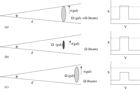
Figure 1: Detectability of galaxies with different column densities in a survey. We consider the case of a galaxy with mass $M_{HI}$ and velocity width $\Delta V$. Panel (a): the galaxy just fills the beam ($\Omega_{beam}=\Omega_{gal}$) and has a peak flux $S$ close to the survey limit (dashed line in the cartoon spectrum on the right hand side). This galaxy will have the lowest detectable column density. In panel (b) the galaxy is smaller, does not fill the beam and has a higher column density. The higher column density compensates for the beam dilution, and the galaxy will still be detected, as shown on the right hand side. Panel (c): as (a) except that the distance $d^{\prime}>d$. The galaxy does not fill the beam, but the low column density yields a peak flux $S$ lower than the survey limit. This galaxy will not be detected.

A more compact galaxy with the same $(M_{HI},\Delta V)$ at the same distance must necessarily have a higher column density (case (b) in Fig. 1). This increase in column density compensates for the beam dilution factor $r_{gal}^{2}/r_{beam}^{2}=\Delta\Omega_{gal}/\Delta\Omega_{beam}$, and the galaxy will still be detected, as its peak flux $S$ is higher than the survey limit.

In contrast, if we take the galaxy from our original example (which just fills the beam at distance $d$) and put it at a larger distance $d^{\prime}$ (case (c) in Fig. 1), the peak flux drops by a factor $(d^{\prime}/d)^{2}$ and will not meet the survey limit.

The detectability of a galaxy is thus independent of its column density, provided that its peak flux is higher than the survey limit. A galaxy filling the beam at the peak flux survey limit will have the lowest detectable column density. At a fixed $(M_{HI},\Delta V)$, galaxies with higher column densities (necessarily) do not fill the beam, but will be detected over the same volume, as they will exhibit identical peak fluxes. Similar galaxies at larger distances will not be detected, independent of column density, as they will drop below the peak flux limit.

Table 2: Volume sampled for galaxies of different masses and column-densities in Mpc³, for a constant velocity width of 200 km s^-1

	$10^{7}M_{\odot}$	$10^{8}M_{\odot}$	$10^{9}M_{\odot}$	$10^{10}M_{\odot}$
$10^{18}$ cm-2	0	0	0	0
$10^{19}$ cm-2	0.22	6.9	220	6900
$10^{20}$ cm-2	0.22	6.9	220	6900
$10^{21}$ cm-2	0.22	6.9	220	6900

Table 2 demonstrates this for galaxies of different masses and column-densities. The $10^{18}$ cm^-2 galaxy is below the column-density limit and will never be detected in HIDEEP. All the other galaxies are above the column-density limit and are therefore detected out to the distances set by their peak fluxes. The volume over which a galaxy above the column-density limit will be detected is determined solely by the peak flux of the galaxy.

In summary, 21-cm surveys have two constraints: (a) a peak-flux limit given by Equation 3 in which dish size ($D$) is a distinct advantage, and (b) a surface-density limit where dish size is irrelevant, but in which integration time per beam is all-important. In a search for high surface-density $N_{HI}$ objects, short integration-times per beam are favoured; in a search for low column-density (and therefore low surface-brightness) objects, long integrations are mandatory. (An alternative way of looking at this is to note that larger dishes project the same system noise on to smaller areas of sky, because their diffraction-limited beams are smaller, and so have to contend with higher apparent sky-noise). Thus HIDEEP and HIPASS are complementary: HIPASS with its relatively short integration-time per beam (450s) picks up large numbers of high surface-density sources but is insensitive to objects below $1.6\times 10^{19}$ cm^-2 ($\Delta V=200$ km s^-1) while HIDEEP with its very long integration-time per beam (9000s) is the first blind survey (see Table 3) capable of reaching much lower surface-density $N_{HI}$, and hence surface-brightness, limits

Before the advent of the multibeam system at Parkes it was neither profitable nor practical to make the very long integrations required to reach low column density. Thus the limits quoted in such surveys for the total amount of cosmic Hi referred only to high column-density clouds and galaxies, though this was rarely acknowledged. Their integration times per beam were mostly far too short to detect the lower surface-density features. HIDEEP (see Appendix B) should and indeed does reach

$$N_{HI}\geq 2.1\times 10^{16}\Delta V$$ (11)

$\simeq 4\times 10^{18}$ cm^-2 for a typical galaxy with a velocity width of 200 km s^-1.

In principle, therefore, we should be able to reach galaxies with lower surface-brightnesses than any detectable before either in Hi or in the optical (see Table 1).

The Hi survey is complemented by deep optical observations, reaching an isophotal level of 26.5 mag arcsec^-2 in the R-band, covering three-quarters of the survey region. For our analysis, we assume a value of $H_{0}=75$ km s^-1 Mpc^-1 throughout.

2 Previous 21-cm Blind Surveys

Despite technical difficulties, blind surveys have been carried out, often using special techniques (see Table 3 for details). For instance Shostak (1977) re-examined the signals in the ‘off-beams’ of an NRAO 300-foot survey, where the ‘on-beams’ were pointed at bright, optically selected galaxies. Latterly, Zwaan et al. (1997) and Schneider, Spitzak, & Rosenberg (1998) have used the Arecibo radio telescope to carry out deep surveys. The results of such blind surveys have generally proved negative in the sense that very few previously-uncatalogued galaxies or intergalactic gas clouds (IGCs) were detected.

Table 3: Blind Hi sureys

	AHISS	Arecibo Slice	Shostak (1977)	Henning (1995)
Telescope	Arecibo	Arecibo	NRAO 300 ft.	NRAO 300 ft.
Channel separation (km s-1)	16	16	11	22
Velocity range (km s-1)	-700 – 7,400	100 – 8,340	-775 – 11,000	-400 – 6,800
Noise channel-1 beam-1 (mJy)	0.75	2	18 – 105	3.4
Ind. Sight-lines	6,000	14,130	6,050	7,200
FWHM	3.3′	3.3′	10.8′	10.8′
Area (deg2)	13	33.6	154	183
$5\sigma M_{HI}$ limit ($M_{\odot}d_{\rm Mpc}^{-2}$)	1.0$\times 10^{5}$	2.8$\times 10^{5}$	2.5 – 15$\times 10^{6}$	4.7$\times 10^{5}$
$5\sigma N_{HI}$ limit (cm-2)d	1.8$\times 10^{19}$	4.8$\times 10^{19}$	4.1 – 24$\times 10^{19}$	7.7$\times 10^{18}$
	ADBS	HIPASS	HIJASS (projected)	HIDEEP
Telescope	Arecibo	Parkes	Lovell	Parkes
Channel separation (km s-1)	33.8	13.2	13.2	13.2
Velocity range (km s-1)	-654 – 7,977	-1280 – 12,700	-3000 – 10,000	-1280 – 12,700
Noise channel-1 beam-1 (mJy)	3 – 4	14	14	3.2
Ind. Sight-lines	181,000	610,000	380,000	670
FWHM	3.3′	15′	12′	15′
Area (deg2)c	430	30,000	13,000	32
$5\sigma M_{HI}$ limit ($M_{\odot}d_{\rm Mpc}^{-2}$)d	4.2 – 5.5$\times 10^{5}$	1.9$\times 10^{6}$	1.9$\times 10^{6}$	4.4$\times 10^{5}$
$5\sigma N_{HI}$ limit (cm-2)d	7.2 - 9.6$\times 10^{19}$	1.6$\times 10^{19}$	2.6$\times 10^{19}$	3.7$\times 10^{18}$

However, as shown in Table 3, such surveys did not have sufficient sensitivity to low column density ($N_{HI}$) gas to actually detect such objects.Quite apart from the theoretical arguments leading to Equation 8, the column-density sensitivity of any survey can be estimated retrospectively from its sensitivity to unresolved sources because (see Appendix C):

$$N_{HI}^{min}(\Delta V)=4.5\times 10^{20}\left(\frac{F_{HI}^{gal}}{\Delta V^{gal}\delta\theta^{2}}\right)^{min}\times\Delta V$$ (12)

where $F_{HI}^{gal}$ and $\Delta V^{gal}$ are the integrated flux (in Jy km s^-1) and the velocity width (in km s^-1) of the source in the survey with the lowest value of $F_{HI}/\Delta V$ and $\delta\theta$ is the source size in arcmin. When considering large LSB galaxies which could fill the beam, we set $\delta\theta$ equal to the beam FWHM to find the sensitivity to such systems. That the left hand side of Equation 12 is independent of dish size can be seen from the right hand side as both the minimum flux (top) and the beam size (bottom) are inversely proportional to the dish area. An examination of the various survey source-limits shows excellent agreement between the column density as calculated according to Appendix C and separately from applying Equation 12 to the various source lists. For instance if we look at the deep drift-scan survey carried out by Zwaan et al. (1997), the Arecibo Hi Strip Survey (AHISS), and examine those sources which lie within its main beam, we can use these to calculate the column-density limit of this survey for a typical velocity width of 200 km s^-1. We find that this limit is:

$$N_{HI}\hbox{(AHISS)}\geq 3.5\times 10^{19}$$ (13)

i.e. $N_{HI}^{lim}$ (AHISS) $\simeq 10^{19.6}$ cm^-2 – almost precisely the minimum value found by the VLA follow-up observations. In other words, the AHISS survey was a shallow survey capable only of picking up sources down to a few times $10^{19}$ cm^-2 with a velocity-width of $\simeq 200$ km s^-1. The AHISS results do not, therefore, rule out the presence of a population of low column-density galaxies. It should be noted that the 5$\sigma$ column-density sensitivity for AHISS given in Table 3 is substantially lower than found in Equation 13. This is consistent with the finding of Schneider et al. (1998) that the limit for AHISS is well above 5$\sigma$.

The other recent deep Arecibo survey, the Arecibo Slice (Schneider et al. 1998; Spitzak & Schneider 1998) operated rather differently. Patches of sky about 2 beam diameters apart were followed for 60s, and any sources tentatively picked up were then re-scanned using a grid search. That meant that the sensitivity varied by a factor of $\simeq 4$ over the total 55 square degrees searched. The median flux of the sources detected over the velocity range 100 to 8340 km s^-1 was 2.69 Jy km s^-1 as against the median value for HIDEEP of 1.96 Jy km s^-1. Because of the short 60s integration time, the sensitivity to low-column-density sources was poorer than AHISS. Nevertheless there were interesting results. Only half the galaxies detected were in any optical catalogue and about a third were LSB galaxies. The galaxies have much lower bulge-to-disc ratios than found in optically-selected samples. The median $M_{HI}/L_{B}$ of the survey was $0.89M_{\odot}/L_{\odot}$ and the galaxies with larger $M_{HI}/L_{B}$ ratios had lower surface-brightnesses.

Henning’s (1992; 1995) survey with the Green Bank 300-foot telescope was largely behind the galactic plane and therefore not comparable with HIDEEP. The Arecibo Dual Beam Survey (ADBS; Rosenberg & Schneider 2000; 2002) covered a larger area of sky than the other surveys but to a much shallower depth, and so could not set any limits to the population of low-column-density galaxies.

Although blind 21-cm surveys are, in principle, the ideal way of circumventing optical selection effects and looking for LSB galaxies and IGCs, the weakness of the 21-cm signal and the system noise make it very difficult to find sources unless they have high column-densities. Only very long integrations are capable of reaching low column-density limits, and possibly finding objects of lower surface-brightness than can be seen optically – thus the interest of HIDEEP. We claim that the arguments summarised in Equation 1 and Table 1 demonstrate that we should, for the first time at 21-cm, be capable of locating such objects. Even so, the limitations of all such blind Hi surveys should constantly be kept in mind. Such surveys have lower sensitivity to broader-line sources (see below) and may, particularly at low column-densities ($<10^{19}$ cm^-2), be severely affected by ionisation and spin temperature effects (Section 4). Hi surveys, therefore, can set only lower limits to the number of LSB galaxies and IGCs in the cosmos.

3 The HIDEEP survey

3.1 The Hi data

HIDEEP was carried out in a region of Centaurus centred on $\alpha=13^{h}40^{m}00^{s}$, $\delta=-30^{\circ}00^{\prime}00^{\prime\prime}$ (J2000) with 1024 spectral channels covering $-1280$ to 12,700 km s^-1. Due to the shape of the Parkes multibeam footprint, the survey has a sensitivity as good as or better than HIPASS over 6 by 10 degrees with a uniform sensitivity over the central 4 by 8 degree area. This region lies in the supergalactic plane, 30 degrees from the galactic plane. The HIDEEP volume includes the Cen A group (Banks et al. 1999) and the outer parts of the Centaurus cluster. The observations were carried out in the southern autumns of 1997, 1998, 1999, and 2000.

The data were processed using the standard multibeam reduction techniques, as described in detail by Barnes et al. (2001). Continuum sources were removed using luther (Wright & Stewart 2003, in preparation). Once integrated, the data take the form of a cube with voxels (3D pixels) 4 by 4 arcminutes on a side and 13.2 km s^-1 deep. The half-power beam width is 15 arcminutes and the data were smoothed in the velocity direction (to reduce ringing) as part of the reduction process, giving a velocity resolution of 18 km s^-1. The data in adjacent voxels are therefore not entirely independent.

The sky was Nyquist sampled 50 times and some 1800 separate samples contributed to the signal in each voxel. Median filtering of this large sample greatly reduces interference while the data were all taken at night to avoid solar radiation entering the beam sidelobes – a major source of noise during the day.

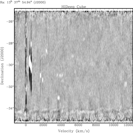
Figure 2: A Decl. – Velocity slice through the HIDEEP cube. At least twelve sources can be seen, including Messier 83 at 500 km s^-1 and GSC 7265 02190 at 11875 km s^-1 (Willmer et al. 1999)

The final data cube can be examined in 3 planes: $(\alpha,\delta)$, $(\delta,V)$ and $(V,\alpha)$, where $V$ is the velocity direction. All 3 planes are used for finding and measuring sources. Figure 2 shows a $(\delta,V)$ slice of the cube, showing the strong galactic signal at 0 km s^-1 as well as 12 other sources including NGC 5236 (M 83) at 500 km s^-1 and GSC 7265 02190 at 11875 km s^-1 (Willmer et al. 1999). Continuum sources have been removed and the nature of the remaining noise, against which sources must be found, can be seen. The ripple seen just below -34^∘ decl. is the residual of the strong continuum from the southern radio-lobe of IC 4296. The increased noise at the edges of the cube is the result of poorer sampling in these regions.

Figure 3: Fall off of noise with integration time. Points are for HIPASS, the intermediate HIDEEP field with 5,600 seconds integration time, and the full HIDEEP field with 9,000 seconds integration time. The line shows the theoretical $1/\sqrt{t_{int}}$ fall-off normalised to the noise in HIPASS.

Figure 3 demonstrates the effectiveness of long integrations. We plot the median noise in mJy beam^-1 channel^-1 for integrations of 450 s beam^-1 (HIPASS), 5,600 s beam^-1 (Minchin 2001) and 9,000 s beam^-1 (HIDEEP). As can be seen it falls to $3.2\pm 0.3$ mJy beam^-1 channel^-1 against time in accordance with the theoretical $1/\sqrt{t_{obs}}$.

Figure 4: Fall off of noise with smoothing. The curves show $N^{0.3}$, $N^{0.4}$ and the theoretical curve from Poisson statistics, $N^{0.5}$ (where $N$ is the number of channels smoothed over).

Figure 4 shows that smoothing in the velocity plane is a much less effective way of reducing the noise. We have smoothed the data with a Hanning filter and removed every other channel from the smoothed cube in order to leave only the independent channels. This has been repeated to form cubes smoothed over 2, 4, 8, 16 and 32 channels. For white noise, the noise should fall as $1/\sqrt{N_{chan}}$ (where $N_{chan}$ is the number of channels smoothed over), however it can be seen that this is not the case for $N_{chan}>4$. Beyond this the fall off is shallower than predicted by Poisson statistics – closer to $N_{chan}^{-0.3}$, although it is not well described by a power-law.

3.2 Source finding

The HIDEEP cube was searched three times in an independent manner. Two different people searched through the cube by eye, inspecting every channel and noting down the sources found, and the third search was carried out by an automated finding routine based on peak-flux detection and template fitting. This routine identified points higher than 4.5-$\sigma$ on a Hanning-smoothed cube and fitted Gaussian templates with a large range of widths at these points, demanding a correlation of better than 0.75. The three lists given by these searches were then compared and any sources found two or more times were accepted. The remaining disputed sources were examined by a third member of the team for a final decision. This team member had not previously searched the data cube.

This gave us a final list of 173 sources, all of which have been judged as real by at least two members of the team acting independently. Accurate positions for all the sources were found by forming zeroth-moment maps around their positions and velocities and fitting Gaussians to these maps. This gives a positional accuracy, as judged from those sources that can be securely identified with optical galaxies, of around 2^′ (see Figure 9). The Hi parameters of the galaxies were measured using the mbspect routine in miriad which provides measures of the velocity width, the noise in the spectrum and the peak flux of the source as well as robust estimates of the integrated flux and systemic velocity.

3.3 Completeness of HIDEEP

The form of the selection present in the HIDEEP survey has been analysed by plotting the integrated flux of the galaxies against their velocity width (Figure 5). For a survey limited solely by the total flux of the galaxies, the selection limit on this graph would be a horizontal line. If the best-possible real-world selection was made, i.e. selection purely by signal-to-noise ratio using optimal smoothing in the velocity plane, then the selection limit would be a line with a slope of 0.5 on a log-log plot (assuming $SNR\propto 1/\sqrt{\Delta V}$, which is not strictly true as shown in Figure 4), shown here as a dashed line. The solid line on the graph shows a selection limit based on peak flux ($F_{HI}\propto\Delta V_{20}$); only 16 of the 173 sources fall below this line and only 8 of these are below by more than 1-$\sigma$. Sources appear to fall further below the line at the low-flux, low-velocity-width end, but this is probably due to the larger errors in this region. The peak-flux selection limit is shown in Figure 6. It can be seen that this explains well the selection limit of the survey.

Figure 5: Selection limits in velocity-width – integrated flux space. The theoretical $5\sigma$ limit for selection based on constant signal-to-noise using optimal smoothing is shown by the dashed line and the $3\sigma$ limit for peak-flux selection ($F_{HI}/\Delta V_{20}=$ constant) is shown by the solid line.

Figure 6: Selection limits in velocity-width – peak-flux space. The $3\sigma$ (9.6 mJy) limit used above can be seen to be a good match to the selection limit of the data. The dashed line shows $\Delta V_{20}$ = 4 channels (52.8 km s^-1).

It can also be seen in both graphs that there is a paucity of galaxies narrower than approximately 4 channel-widths (52.8 km s^-1). This further selection effect, thought to be due to galaxies narrower than this being indistinguishable from interference, is investigated in detail by Lang et al. (2003).

The completeness of the HIDEEP catalogue has been calculated by looking at how the source counts vary with peak flux, as shown in Figures 7 and 8. For this analysis, 41 sources that may have been detectable beyond the upper velocity limit were excluded in order to make a purely flux-limited sample. It can be seen from both figures that the peak flux completeness limit is 18 mJy, or around 5.5$\sigma$. This is around the level where the completeness limit is expected to fall. It can also be seen that large numbers of sources are found between the completeness limit at 18 mJy and the selection limit of $\simeq 10$ mJy.

Figure 7: Completeness of the HIDEEP survey: Source count against peak flux ($S_{peak}$). The histogram shows numbers found in each bin of peak flux, the curve represents $N(S_{peak})\propto S_{peak}^{-5/2}$ as expected for a flux-limited survey.

Figure 8: Completeness of the HIDEEP survey: Log-log plot of source count against peak flux. The solid line has a slope of $-3/2$, as expected for a flux-limited survey.

3.4 The optical data

To identify LSB galaxies it was necessary to obtain very deep optical data to compare with the radio. Accordingly eight 1-hour $6^{\circ}\times 6^{\circ}$ R-band Tech-Pan films were exposed at the UK Schmidt Telescope, centred on $13^{h}39^{m}50^{s}$ ,$-30^{\circ}00^{\prime}12^{\prime\prime}$ (J2000). These were digitised, linearised and stacked using the SuperCOSMOS machine at the UK Astronomical Technology Centre in Edinburgh (Hambly et al. 2001). The final image was then calibrated using the magnitudes of unsaturated ESO-LV (Lauberts & Valentijn, 1989) galaxies within the region, which yields a calibration accuracy of approximately 0.2 magnitudes. The Tech-Pan films used go 1 mag deeper than the IIIaF plates previously used at the UKST (Parker & Malin 1999) and the digital stacking gives a further gain of over a magnitude compared to a single exposure (Schartzenberg, Phillipps, & Parker, 1996). The limiting surface-brightness reached for small objects within the image is then 26.5 R mag arcsec^-2, equivalent to between 27 and 28 B mag arcsec^-2.

Within the overlap region between the radio and optical images we find 96 Hi sources which have been uniquely identified with optical counterparts.

Sources have been identified with galaxies on the optical image, firstly on the basis of positional coincidences. Multibeam survey positions are generally accurate to 2 arcminutes (Koribalski et al. 2003), but this can be checked for the 65 optical counterparts which have previously published optical velocities or for which we have our own optical spectroscopy or 21-cm interferometry data. A comparison can be made between the (radio – optical) offsets of these firm detections with the remainder (Figure 9). A Kolmogorov-Smirnov test confirms that there is no significant difference between the distributions, implying that the purely positional coincidences can generally be trusted. There may still be one or two incorrect identifications, but the tail of offsets out to 6.5 arcminutes probably reflects the positional accuracy of the HIDEEP survey.

Figure 9: Comparison between the cumulative distributions of offsets for the firm identifications (solid line) and the less certain counterparts (dashed line).

In the overlap area 59% of the sources are identified with previously catalogued galaxies with matching redshifts, 24% with previously catalogued galaxies without redshifts, and 17% are previously uncatalogued galaxies. It appears that there are no intergalactic gas clouds unassociated with optical counterparts: all those galaxies which have not been uniquely associated with a counterpart have more than one plausible candidate.

Figure 10: Number of galaxies found in each surface-brightness bin. The solid line shows the distribution of observed surface-brightnesses, the dashed line shows the distribution of surface-brightnesses after correction for galactic absorption, cosmological dimming, and inclination.

We have measured effective radii and surface-brightnesses by fitting to the surface-brightness profiles of the optical sources using the ellipse routine in IRAF. The total magnitudes used were determined by sextractor (Bertins & Arnouts 1996). The surface-brightness distribution (Figure 10) is much broader than one finds in optically selected samples. A Kolmogorov-Smirnov test of our distribution and the surface-brightness distribution of the ESO-LV shows that the hypothesis that both are drawn from the same parent population has a significance of less than 1% – this is due to the larger number of LSB galaxies seen in the HIDEEP sample. This confirms that Hi surveys do, as expected, avoid some of the surface-brightness selection effects present in optical surveys. A fuller description and analysis of the optical properties will be given in a second paper (Minchin et al. 2003, in preparation).

3.5 Internal Hi correlations

A correlation between Hi mass and observed velocity width of the form $\Delta V\propto M_{HI}^{\beta}$ (where $\Delta V$ is the velocity width uncorrected for inclination) is expected in the HIDEEP data as it has been seen in optically-selected samples (e.g. Briggs & Rao 1993) and as it would be the consequence of the Hi Tully-Fisher relationship.

Figure 11: Hi mass – velocity width relationship for HIDEEP sources. The best fit to the HIDEEP data ($\Delta V=0.42^{+0.30}_{-0.17}M_{HI}^{0.282\pm 0.025}$) is shown by a solid line, while the fit of $\Delta V=0.15M_{HI}^{1/3}$ (Briggs & Rao 1993) is shown as a dashed line.

That such a relationship can be seen in the HIDEEP data is shown in Figure 11. The solid lines shown here is for the best fit of $\Delta V_{20}=0.42^{+0.30}_{-0.17}M_{HI}^{0.282\pm 0.025}$ . The dashed line shows $\Delta V=0.15M_{HI}^{1/3}$ as found by Briggs & Rao (1993). The best-fit slope found for the HIDEEP data is $2\sigma$ shallower than this, however this may be due to the selection against narrow velocity-width galaxies seen earlier. We cannot, therefore, conclusively say that our sample shows a different relationship to that found by Briggs & Rao.

It is also expected that there will be a relationship between peak flux and the value of $F_{HI}/\Delta V_{20}$ – the peak flux of a top-hat function with a width of the 20% width of the source and containing the same total flux. This relationship is important for calculated Hi mass limits in a peak-flux limited survey, as it is necessary for relating the peak-flux limit to the integrated flux ($F_{HI}$) on which the Hi mass depends.

Figure 12: Comparison of the ratio $\frac{S_{peak}}{F_{HI}/\Delta V}$ with $M_{HI}$. The slope of the best-fit to this data is indistinguishable from zero, we therefore use the median value, $1.7\pm 0.3$ to describe the ratio across all Hi masses.

However, as this relationship depends on the profile shape it may well vary with Hi mass. This is investigated in Figure 12. This figure shows that there is no dependence of the ratio $\frac{S_{peak}}{F_{HI}/\Delta V}$ on $M_{HI}$: the slope of a fit to the points is statistically indistinguishable from zero. We therefore take the ratio to be a single number for all Hi masses, using the median value: $1.7\pm 0.3$. This value was used to calculate the $3\sigma$ peak-flux limit in Figure 5.

Figure 13: Distribution of Hi masses. The solid line shows the distribution for the whole survey, the dashed line shows the distribution excluding galaxies in the Centaurus A group and the dotted line shows the distribution of galaxies included in the optical sample.

The Hi mass distribution of the HIDEEP sources is shown in Figure 13. This shows both the distribution of all the sources in HIDEEP (solid line), the distribution if the Centaurus A group galaxies are ignored (dashed line) and the distribution of galaxies included in the optical sample (dotted line). It can be seen that most of the low-mass galaxies are, unsurprisingly, in the Centaurus A group but we find only one high-mass galaxy (Messier 83). There are 22 hydrogen giants with $M_{HI}>10^{10}M_{\odot}$, but only NGC 5291 has a mass greater than $3\times 10^{10}M_{\odot}$. There are no galaxies detected outside the range $10^{6}M_{\odot}<M_{HI}<10^{11}M_{\odot}$. The optical sample is similar in shape to the full sample, but contains fewer sources. This is mainly because it covers a smaller area. Some sources have also been omitted as a unique optical counterpart could not be identified.

3.6 Sensitivity and comparisons with previous surveys

Using the completeness limits and relationships found in the Hi data, we can calculate the sensitivity limit of the HIDEEP survey to galaxies of different masses and different column-densities. The mass (in solar masses) is related to the integrated flux by the equation

$$M_{HI}=2.356\times 10^{5}F_{HI}d_{Mpc}^{2}$$ (14)

(for $F_{HI}$ in Jy km s^-1) and the total flux is related to the peak flux and the velocity width (Figure 12) by

$$S_{peak}=(1.7\pm 0.3)\times\frac{F_{HI}}{\Delta V_{20}}$$ (15)

This allows the mass to be related to the peak flux as:

$$M_{HI}\simeq 1.386\times 10^{5}S_{peak}\Delta V_{20}d_{Mpc}^{2}$$ (16)

However the velocity width is a function of the mass, $\Delta V\simeq 0.15M_{HI}^{1/3}$ (although with a large scatter). If we use the relationship found by Briggs & Rao (1993) then

$$M_{HI}\simeq\left(0.15\times 1.386\times 10^{5}S_{peak}d_{Mpc}^{2}\right)^{3/2}$$ (17)

which gives:

$$M_{HI}\simeq 3.0\times 10^{6}S_{peak}^{3/2}d_{Mpc}^{3}$$ (18)

and putting in the completeness limit of $S_{peak}=0.018$ Jy gives:

$$M_{HI}\simeq 7.24\times 10^{3}d_{Mpc}^{3}$$ (19)

which is the sensitivity limit for sources of different masses at different distances. Since the relationship between velocity-width and mass has a large scatter this is not the absolute detection limit: sources narrower than predicted by this relationship will be seen further out, and sources wider than predicted will be found over a smaller volume. However, it does indicate the distance to which most sources of a given mass will be seen.

The relationship between mass and velocity-width suggests the possibility of a selection effect in Hi surveys that appears to have been neglected in many previous surveys: that of a minimum believable velocity width. Below a certain mass, the velocity-widths of many of the galaxies will be smaller than the minimum believable velocity-width of the survey – the width at which a peak in the data is recognised to be a galaxy rather than a noise peak – and will not be catalogued. A fuller analysis of this effect, using data from the Hi Jodrell All Sky Survey, is given in Lang et al. (2003).

Examination of the HIDEEP data shows the minimum believable velocity-width to be around 4 channels wide for $\Delta V_{20}$, or 52.8 km s^-1. This selection effect means that detecting large numbers of low-mass galaxies will require not only sensitivity but also narrow channel-widths. However, this effect could remove at most $\sim 40$ per cent of $10^{7}M_{\odot}$ galaxies here. If the thermal broadening of the Hi is also taken into account, this percentage will fall. It is therefore unlikely that this will significantly change the shape of Hi mass functions down to their current mass limits. For HIDEEP, the distance at which galaxies that would be above the mass limit will fall below the minimum believable velocity-width limit is about 18 Mpc.

Figure 14: Hi mass limits for three surveys: HIDEEP (solid line), the HIPASS Bright Galaxy Catalogue (BGC; dotted line) and the Arecibo Hi Strip Survey (AHISS; dashed line).

Figure 14 compares the Hi mass sensitivity of three surveys: HIDEEP, the HIPASS Bright Galaxy Catalogue (Koribalski 2003; BGC) and the Arecibo Hi Strip Survey (AHISS). A minimum believable velocity-width of 4 channels has been applied to all these surveys although galaxies narrower than this can be seen if they have high peak signal to noise ratios. This will apply particularly to the HIPASS BGC, where the peak-flux cutoff of 116 mJy is more than 8$\sigma$. For AHISS a limit of 5.25 mJy, or seven times the stated noise value of 0.75 mJy per channel, was adopted. This appears consistent with an analysis of the fluxes and velocity widths from Zwaan (2000) and with the analysis of Schneider et al. (1998) which concluded that the AHISS survey was limited at 7$\sigma$ due to the method of confirming sources. Only the primary beam area was used in calculating the volume covered by AHISS.

Having estimated the sensitivity to sources in the mass-limited regime, we can also estimate the sensitivity to sources in the column-density limited regime. Column-density sensitivity has often been presented, in a similar manner to optical surface-brightness, as not having a dependence on distance. However the relationship between $\Delta V$ and $M_{HI}$ and the dependence of column-density sensitivity of $\Delta V$ (see Equation 12) means that this is not the case for single-dish surveys – the tendency of higher mass sources to have larger velocity widths means that they will (a) be seen to greater distances due to their higher mass and (b) will have a higher column-density limit due to their larger velocity width.

The column-density of a source filling the beam (in $M_{\odot}$ pc^-2) is given by:

$$N_{HI}=\frac{M_{HI}}{\pi\theta^{2}d^{2}_{pc}}M_{\odot}\hbox{ pc}^{-2}$$ (20)

where $\theta$ is the HWHM of the telescope beam in radians and $d_{pc}$ is the distance of the source in parsecs. It can easily be seen that $N_{HI}$ is only independent of distance if the sensitivity of the telescope to $M_{HI}$ goes as $d^{2}$. This would only be the case if galaxies at all different Hi masses had the same velocity-width or if the survey was limited by integrated-flux – neither of which are likely. There must, therefore, be a distance dependence for column-density sensitivity to average galaxies which follow the relationship between $M_{HI}$ and $\Delta V$.

Putting in the $M_{HI}$ sensitivity from Equation 19 and the beam size of Parkes (15 arcmin) gives a column-density sensitivity for HIDEEP of:

$$N_{HI}\simeq 6.1\times 10^{16}d_{Mpc}\hbox{ cm}^{-2}$$ (21)

Figure 15: Hi column-density limits for three surveys: HIDEEP (solid line), the HIPASS Bright Galaxy Catalogue (BGC; dotted line) and the Arecibo Hi Strip Survey (AHISS; dashed line). It can be seen that HIDEEP is considerably more sensitive than previous surveys to low column-density sources.

Again, this will be affected by the minimum believable velocity-width limit. Column-density limits for the three surveys (HIDEEP, HIPASS BGC and AHISS) are given in Figure 15 where it can be seen that HIDEEP has a considerable advantage.

Figure 16: Coverage of $M_{HI}$ – $N_{HI}$ space for three surveys: HIDEEP (solid line), the HIPASS Bright Galaxy Catalogue (BGC; dotted line) and the Arecibo Hi Strip Survey (AHISS; dashed line). This shows that neither the HIPASS BGC nor the AHISS were likely to find low surface-brightness giant galaxies. However, if these exist and are not very rare, they should be found by HIDEEP.

Figure 16 shows the region of $M_{HI}$ – $N_{HI}$ space in which each survey is sensitive. HIDEEP extends the region of $M_{HI}$ – $N_{HI}$ space explored. For instance, neither the HIPASS BGC or AHISS would find giant LSB galaxies unless they had very high $(M_{HI}/L_{B})$s or very low velocity widths.

3.7 Hi properties

The Hi properties of a sample of HIDEEP sources are given in Table 4 (full table available online). Column 1 gives the HIDEEP identification for the source. Columns 2 and 3 give the right ascension and declination from fitting to the zeroth-moment map. Columns 4 – 6 give the noise as measured on the part of the spectrum not containing signal ($\sigma$), the integrated flux (zeroth-moment, $F_{HI}$), and the peak flux ($S_{peak}$), all as measured by mbspect. Columns 7 and 8 give the systemic heliocentric velocity (first-moment, $V_{\odot}$) and the velocity width at 20% of the peak flux ($\Delta V_{20}$), measured by mbspect in the radio-velocity frame ($c\frac{\Delta\nu}{\nu}$) and converted to $cz$. Column 9 gives the distance in Mpc calculated from the CMB rest-frame velocity of the sources, which is approximately $V_{CMB}=V_{\odot}+278\pm 8$ km s^-1 for the HIDEEP region (the exact correction varies across the field). This does not include any correction for bulk-motions (Virgo-centric infall, etc.) nor does it include assigning sources beyond the Centaurus A group to clusters and assigning a single distance to that cluster. Galaxies at less that 1000 km s^-1 have been assigned to the Centaurus A group at an assumed distance of 3.5 Mpc. Column 10 gives the Hi mass calculated from $F_{HI}$ from column 5 and the distance from column 9 using the standard equation $M_{HI}=2.356\times 10^{5}F_{HI}d^{2}_{Mpc}M_{\odot}$, where $F_{HI}$ is in Jy km s^-1.

3.8 Large-scale structure

The HIDEEP survey region lies in the supergalactic plane and there is, therefore, much large scale structure in the survey volume. This can be seen in Figure 17. In particular, the Centaurus A group, the Virgo Southern Extension and the Centaurus Cluster can be seen. Near the end of the bandpass a number of Abell clusters are found, and more lie beyond the outer velocity edge of our survey.

Figure 17: Large scale structure of galaxies detected in HIDEEP (filled circles). These pie-slices show the distribution in R.A. (upper) and Decl. (lower), with the angle expanded by a factor of three for clarity. Galaxies from NED (crosses) are included for comparative purposes, it can be seen the Hi selected sample traces approximately the same large scale structure.

Figure 18: Hi sources and galaxies in NED between 10,000 km s^-1 and the HIDEEP bandpass limit of 12,700 km s^-1. The previously catalogued galaxies with redshifts are shown as dots and the HIDEEP sources are shown as filled circles. Abell cluster numbers are superimposed on the concentrations of galaxies using positions from Abell, Corwin, & Olowin (1989), these have been shifted 0.75 degrees south for the sake of clarity.

Figure 18 shows that there is little correlation between the distribution of previously catalogued galaxies with redshifts above 10,000 km s^-1 and the distribution of the HIDEEP sources in this velocity range. Only the Abell 3562 cluster appears to have a significant number of Hi detections and the Hi sources also appear to populate the void at the north-west of the region. It is possible that the lack of correlation is due to the targeting of optical redshift surveys towards the Abell clusters, thus increasing the number of redshifts in those regions out of proportion to their density. While Abell 3571 and 1736 are both centred inside the HIDEEP volume, at 11,500 km s^-1 and 10,500 km s^-1 respectively, Abell 3558 and 3562 are both centred beyond 14,000 km s^-1 (Abell, Corwin, & Olowen 1989; Quintana & de Souza 1993). Only the low-velocity tails of these two clusters can be seen.

3.9 Follow-up observations

Follow up observations of some sources were carried out at 21-cm using the Australia Telescope Compact Array (ATCA) and optically using the Double Beam Spectrograph on the ANU 2.3-m telescope at Siding Spring Observatory. The ATCA observations were carried out in the 375-m configuration in November 1999 and January 2000 and gave us high-resolution 21-cm maps of the targeted sources in order to accurately determine their positions. Ten out of fourteen sources were detected. As the column-density sensitivity limit for these observations was around $10^{21}$ cm^-2, substantially higher than the limit for the HIDEEP survey, the non-detections do not tell us anything about our survey limits.

Optical spectroscopy has enabled us to positively identify ESO 509-G075 as the counterpart of HIDEEP J1335-2730 (which was undetected with ATCA) despite a previous optical redshift (Quintana et al. 1995) placing it at twice the velocity of the Hi source and allowed us to seperate Abell 3558:[MGP94]4312 and 4317 which were too close together to be separated by ATCA, identifying 4317 as the optical counterpart of HIDEEP J1334-3223.

4 Inferred Hi Column-Densities

We have not yet obtained high-resolution Hi images of most of our sources so we do not know either their Hi radii or column densities. We therefore calculate an inferred column-density ($N_{HI}^{\circ}$) from the Hi mass and the optical (effective) radius. Because of our long integration time and low noise, we could in principle reach column densities between one and two orders of magnitude deeper than previous blind surveys (Section 2). It is of interest to look for evidence, however indirect, as to whether this previously unexplored parameter space is populated.

Salpeter and Hoffman (1996) found that $r_{HI}=(2.34\pm 0.14)\times r_{B25}$ for an optically-selected sample of galaxies. Obviously $r_{B25}$ is not a good measure for the Hi radii of LSB galaxies, which may not have a $B_{25}$ isophote. However, the effective radius ($r_{e}$) provides a model and surface-brightness independent measure of the optical size of galaxies. In order to obtain a relationship between $r_{e}$ and $r_{HI}$, it is necessary to assume a relationship between $r_{B25}$ and $r_{e}$. This obviously introduces some unavoidable model-dependency into the analysis. As the relationship between $r_{HI}$ and $r_{B25}$ is defined for HSB galaxies, we should define the relationship between $r_{e}$ and $r_{B25}$ for a similar sample. There is a further assumption here that the proportionality between $r_{e}$ and $r_{HI}$ found for these HSB galaxies will remain constant as we go to lower surface-brightnesses. This may not be the case, and would introduce systematic errors into our analysis, however $r_{e}$ is certainly a better choice that $r_{B25}$ for looking at LSB galaxies. We use the relationship for disc galaxies in the ESO-LV catalogue (Lauberts & Valentijn 1989) that $r_{B25}=(2.15\pm 0.67)\times r_{e}^{B}$. This then gives us:

$$r_{HI}=(5.03\pm 1.59)\times r_{e}^{R}$$ (22)

From this we can calculate the inferred mean column-density $N_{HI}^{\circ}$ as:

$$N_{HI}^{\circ}=10^{20.1}\frac{M_{HI}}{\pi R_{HI}^{2}}\hbox{ cm${}^{-2}$}$$ (23)

where $R_{HI}$ is the radius in pc, calculated from $r_{HI}$ using the distance to the source.

Figure 19: Inferred column-densities of HIDEEP sources against velocity widths. The limit shown is for the 18 mJy completeness limit for HIDEEP and sources filling the beam.

Figure 19 shows these inferred column-densities plotted against their velocity widths. Above the survey limit (dashed line), the volume sampled depends only on Hi mass (or, more precisely, on peak flux) and not on column-density, as shown earlier in Figure 1. If low column-density galaxies were common, we would expect to see galaxies at all column-densities in this plot. However, this is clearly not the case – there is a large gap between the lowest column-density galaxies found and our sensitivity limit.

Figure 20: Inferred column-densities of HIDEEP sources with different beam filling factors against velocity widths. The limits shown are for the 18 mJy HIDEEP completeness limit, the dotted line indicating the limit for the lower filling factor and the solid line the limit for the higher filling factor in each subgraph.

That this gap is real and not an artefact of our method is shown in Figure 20. Here the sample has been split into four sections, according to the beam-filling factor ($\Delta\Omega/\Omega_{beam}$) of the sources, and the column-density limits calculated with this included. The top left panel shows that we are detecting galaxies up to the column density limit of the survey for this range in beam filling factors. These are galaxies with small beam-filling factors, and we can see that the inferred column density limits for these galaxies are quite high (cf. Eqn B6). The top right panel shows the limits for galaxies with slightly larger beam filling factors. Galaxies are detected with column densities close to the survey limit for this range in beam filling factors, but we can see that they do not approach the limit as closely as in the previous panel. This is an indication that in this sample galaxies with larger beam filling factors (and hence lower column densities; cf. Sect. 1) are rarer. This is confirmed by the two bottom panels. These show the limits for galaxies that come close to filling the beam (and thus have the lowest column densities). We see that despite the low limits, there are only two galaxies detected. This thus indicates an absence of low-column density galaxies, despite their potential detectability.

Using the numbers of galaxies found within the overlap of the full-sensitivity Hi survey and the optical survey, we calculate that, to 95% confidence, low column-density galaxies make up less than 21% of galaxies with Hi masses between $10^{8}$ and $10^{9}M_{\odot}$ (13 galaxies), less than 6% between $10^{9}$ and $10^{10}M_{\odot}$ (52 galaxies), and less than 19% between $10^{10}$ and $10^{11}M_{\odot}$ (14 galaxies).

If our estimate of $R_{HI}$ were out by more than a factor of three, we would expect to see a lower limit to our column densities parallel to the plotted completeness limit. As the lower limit appears flat with respect to velocity width, it appears that there are indeed no large very low column-density galaxies in our sample. If such objects are present in the local Universe they must, therefore, be rare. We discuss possible reasons for this absence elsewhere (Disney & Minchin 2003).

Figure 21: Distribution of inferred column-densities of HIDEEP sources. The dashed line indicates a Gaussian with a mean of 20.65 and a scatter of 0.38. It can be seen that this is a fairly good description of the distribution.

The distribution of column densities appears to be the same at all surface brightnesses. A two-dimensional Kolmogorov-Smirnov test (Peacock 1983) shows that the observed distribution is indeed consistent with a distribution having the same column-density distribution as HIDEEP (Fig. 21) at every surface brightness. The distribution shown in Figure 21, is well described by a Gaussian with $\log(N_{HI}/\hbox{cm}^{-2})=20.65\pm 0.38$. Figure 22 shows the measured data which gives rise to a constant column-density: a relationship between the effective radius and the Hi flux. The dashed line on this graph is for a constant $N_{HI}^{\circ}$ of $10^{20.65}$ cm^-2, and it can be seen that this matches the data well. This apparent constancy of column density is unexpected, we would expect to see a fall-off towards lower surface-brightness, as observed by de Blok et al. (1996) for a sample of LSB galaxies observed with the Westerbork Synthesis Radio Telescope (WSRT).

Swaters et al. (2002) observed a number of optically-selected galaxies with the WSRT, showing that the relationship between Hi mass and diameter was much tighter when true Hi diameters were used than when they were inferred from the optical radii. It is likely that much of the scatter in our relationship has been similarly introduced by our use of optical radii. Observations of the true Hi diameters may well show a similar trend to that seen by de Blok et al.

Figure 22: Relationship between effective radius and Hi flux. The dashed line shows the expected slope for $N_{HI}^{\circ}=10^{20.65}$ $cm^{-2}$.

In order to compare our sample with the literature, we have taken the LSB galaxy catalogue of Impey et al. (1996; ISIB96). This survey provides effective surface-brightnesses and radii for all the galaxies found, across a wide range of surface brightness, and provides Hi mass measurements for a subsample of 190 galaxies. We therefore calculate the column density from this data in exactly the same manner as for HIDEEP. The Impey et al. survey was carried out in B-band, we therefore convert $\mu_{e}^{B}$ to $\mu_{e}^{R}$ using the average colour for disc galaxies from de Jong 1996, $B-R=1.1$.

Figure 23: Comparison between the surface-brightness – column-density distribution for HIDEEP (triangles) and Impey et al. (1996), converted to R-band assuming $B-R=1.1$ (open circles). Error bars have been omitted for the sake of clarity.

Figure 23 shows the surface-brightness – column-density distribution for both surveys. HIDEEP galaxies are indicated by solid triangles, ISIB96 galaxies by open circles. It can be seen that there is a clear trend in the ISIB96 data, which is similar to that seen by de Blok et al. (1996). The surface-brightness distribution of the ISIB96 galaxies is different to that of HIDEEP, due to the method in which the galaxies have been selected. In order to compare the surveys we have therefore re-sampled the ISIB96 data to give the same surface-brightness distribution (in 0.5 mag bins) as HIDEEP. This was carried out ten times, and the subsamples compared with HIDEEP using the two-dimensional Kolmogorov-Smirnov test. Half of the subsamples were not significantly different at the 95% level.

There are a number of systematics that could affect this comparison. Our measure of $r_{e}$ could be systematically too small towards lower surface-brightnesses: this would lead to both $N_{HI}^{\circ}$ and $\mu_{e}$ being higher and so would act to destroy such a relationship between $N_{HI}$ and surface-brightness. The colours will not be exactly the same for all the galaxies, introducing errors into the conversion of the ISIB96 relationship to R-band. The low column-density galaxies ($N_{HI}^{\circ}<10^{20}$ cm^-2) in ISIB96 are generally large galaxies, with $r_{eff}>20^{\prime\prime}$. Using our scaling between $r_{HI}$ and $r_{eff}$, this gives them Hi sizes larger than the Arecibo beam. It is therefore likely that some of the hydrogen in these galaxies was missed in the pointed observations, leading to lower inferred column-densities than is truly the case. We cannot, therefore, say that the HIDEEP data is inconsistent with ISIB96. If there is a relationship between surface-brightness and $N_{HI}$ in our data, however, it is very weak indeed.

5 Discussion, Conclusions and future work

The existence of a large population of LSB galaxies could have a significant impact on several areas of astronomy, in particular on measurements of the luminosity and mass density of galaxies and on theories of galaxy formation and evolution. However, LSB objects are difficult to detect in the optical since, by definition, they are hard to discriminate from the background sky. Hence, alternative techniques need to be considered for determining whether there exists a significant population of extragalactic objects with optically LSB. Searches for galaxies using the 21-cm line of atomic hydrogen provide one such alternative method. If LSB galaxies have similar hydrogen content to galaxies of higher surface brightness, then we might expect that a 21-cm survey will not be biased against LSB galaxies.

However, the detection of a galaxy in a 21-cm survey is a function of both its Hi column density and its Hi mass. If a galaxy has a column density below the column density limit of the survey then it will never be detected whatever its total Hi mass. Assuming LSB galaxies have similar Hi content to brighter galaxies but that this is distributed over a larger surface area, then we would expect LSB objects to have lower Hi column densities. Previous Hi surveys have not generally had long enough integration times to search to sufficiently low column densities to draw definite conclusions about the cosmic prevalence of gas-rich LSB galaxies. HIDEEP with its 9000s beam^-1 integration time is the first survey with sufficient column density sensitivity to be able to place interesting limits on the existence and size of a low column-density/LSB population. Two major conclusions from HIDEEP have been presented here.

Firstly, all of the sources found in HIDEEP appear to be associated with an optical counterpart on our deep UK Schmidt R-band data. In other words, we have not found an intergalactic Hi cloud down to our observational column density limit of N_HI/$\Delta$V = 2.1$\times$10¹⁶ cm^-2 which corresponds to an N_HI of 4.2$\times$10¹⁸ cm^-2 for a typical galaxy velocity-distribution ($\Delta$V=200 km s^-1) and 3.2$\times$10¹⁷ cm^-2 for a typical QSOAL dispersion (15 km s^-1). Wherever neutral hydrogen is found it is accompanied by a visible population of stars above our surface-brightness limit of 26.5 R magnitudes per square arcsecond ($\sim$27.5 in B).

Secondly, if we infer the Hi sizes of the HIDEEP detections from their optical sizes, then we can derive Hi column densities for them. These derived column densities are all $\ga$10²⁰ cm^-2, more than an order of magnitude above our observational limit. Assuming that our method of inferring Hi size from optical size is robust, then this result implies that there is no significant population of galaxies with Hi column densities $\la$10²⁰ cm^-2. We are currently undertaking a VLA and ATCA survey of all the HIDEEP sources in order to measure their column densities directly. This will enable us to test this result without having to infer Hi size from optical size.

Possible physical explanations for this intriguing second result are discussed in detail elsewhere (Disney & Minchin 2003). Ionisation is unlikely to be responsible since the intergalactic radiation field locally is at least an order to magnitude too small (Scott et al. 2002). Another possibility, raised in the early days of 21-cm astronomy, is ‘freezing out’ – i.e. that the 21-cm spin temperature of low column density objects may fall to the cosmic background temperature, rendering such clouds invisible in emission.

The cosmic significance of gas-rich low-surface brightness galaxies will be the subject of a subsequent paper based on this same data (Minchin et al. 2003, in preparation). However, the fact that we have not found a single galaxy in Hi which cannot be seen in our optical data suggests that there cannot be large numbers of gas-rich extremely LSB galaxies or intergalactic clouds.

If our second result is confirmed by the follow-up VLA and ATCA observations, then this will imply that Hi surveys need not have column density limits much lower than $\sim$10²⁰ cm^-2, since few galaxies would appear to have column densities lower than this. In particular, this would imply that previous large-area, shallow surveys, e.g. HIPASS and HIJASS, will not have missed many low-column density objects. However, long integrations using telescopes with smaller beams would improve the statistics on the numbers of low mass, low column-density sources.

Appendix A Derivation of the surface-brightness – column-density relation

For any given area the Hi surface density and the optical surface brightness are related by:

$$\Sigma_{HI}\left(M_{\odot}\hbox{pc}^{-2}\right)=\left(\frac{M_{HI}}{L_{B}}\right)\times\Sigma_{B}\left(L_{\odot}\hbox{pc}^{-2}\right)$$ (24)

where $\Sigma_{HI}$ is the Hi surface density and $\Sigma_{B}$ is the B-band optical surface brightness, averaged over the region, and $M_{HI}$ and $L_{B}$ are the Hi mass and the B-band luminosity within the same region. As 1 $M_{\odot}$ pc^-2 is approximately equal to an Hi column density of 10^20.1 cm^-2 and 1 $L_{\odot}$ pc^-2 is approximately equal to a surface-brightness of 27.05 B mag arcsec^-2, this gives the scaling relationship:

$$N_{HI}\simeq 10^{20.1}\left(\frac{M_{HI}}{L_{B}}\right)10^{\left(0.4\left(27-\mu_{mean}\right)\right)}$$ (25)

where $N_{HI}$ is the Hi column density in units of cm^-2 and $\mu_{mean}$ is the average optical surface brightness in units of mag arcsec^-2 taken over the same area as $N_{HI}$. This can be re-written as:

$$\mu_{mean}\simeq 2.5\left(30.1+\log\left(\frac{M_{HI}}{L_{B}}\right)-\log\left(N_{HI}\right)\right)$$ (26)

This relation can be adapted to relate the central surface-brightness of a galaxy to its average Hi column density if certain assumptions are made about the size of the Hi disc. Cayatte et al. (1994) found that $R_{HI}\simeq 1.7R_{25}$. This scaling will obviously not hold for LSB galaxies, some of which may not even have a $\mu_{B}=25$ isophote, but for a Freeman’s law galaxy $R_{25}=3.1$ scale lengths and it therefore seems reasonable to assume that $R_{HI}=3.1\times 1.7=5.25$ scale lengths. Assuming also that $M_{HI}/L_{B}=0.3M_{\odot}/L_{\odot}$ (average value from Roberts & Haynes 1994), we get:

$$\mu_{0}\simeq 2.5\left(28.95-\log\left(N_{HI}\right)\right)$$ (27)

which can be used to work out an approximate equivalent central surface-brightness limit for Hi surveys.

Appendix B Column-density sensitivity

The signal entering the receiver is measured in terms of the antenna temperature $T_{A}$ where

$$kT_{A}=S_{\nu}D^{2}$$ (28)

$S_{\nu}$ is the strength of the source in flux units and $D$ the dish-diameter. For a significant detection $T_{A}$ should exceed the uncertainty in the system power by some signal-to-noise-ratio $\sigma$, i.e.

$$T_{A}\geq\sigma\frac{T_{sys}}{\sqrt{t_{int}\Delta\nu}}$$ (29)

which is the usual ‘antenna equation’ derived from the bandwidth theorem.

In the Rayleigh-Jeans regime, surface brightness is conventionally expressed in terms of the brightness temperature

$$T_{B}=\frac{\lambda^{2}}{2k}\frac{S_{\nu}}{\Delta\Omega}$$ (30)

where $\Delta\Omega$ is the solid angle of the source. For Hi galaxies quantum mechanics yields

$$\frac{N_{HI}}{\Delta V}=1.8\times 10^{18}T_{B}$$ (31)

where $N_{HI}$ is the column-density in cm^-2 and $\Delta V$ is the velocity width of the line.

The antenna equation (29) can now be rewritten as

$$\frac{N_{HI}}{\Delta V}>1.8\times 10^{18}\frac{\lambda^{2}}{2D^{2}\Delta\Omega}\frac{\sigma T_{sys}}{\sqrt{t_{obs}\Delta\nu_{ch}}}$$ (32)

where we have replaced $\Delta\nu$ with $\Delta\nu_{ch}$ because we are here interested in a peak-flux limited survey.

If we now substitute in the beam size, $\Omega_{b}=1.13(\lambda/D)^{2}$, and the channel velocity-width $\Delta V_{ch}=(c/\nu_{rest})\times\Delta\nu_{ch}$, we get

$$\frac{N_{HI}}{\Delta V}\geq 5.5\times 10^{16}\frac{\Omega_{b}}{\Delta\Omega}\frac{\sigma T_{sys}}{\sqrt{t_{obs}\Delta V_{ch}}}$$ (33)

So, if the source fills the beam, i.e. $\Omega_{b}/\Delta\Omega=1$

$$\frac{N_{HI}}{\Delta V}\geq 5.5\times 10^{16}\frac{\sigma T_{sys}}{\sqrt{t_{obs}\Delta V_{ch}}}$$ (34)

which agrees with Equation 8, and is indeed independent of telescope diameter. For HIDEEP, $T_{sys}=26$K, $t_{obs}=9000$s, $\Delta V_{ch}=13.2$ km s^-1 and if $\sigma=5$

$$\frac{N_{HI}}{\Delta V}\geq 2.1\times 10^{16}\hbox{cm${}^{-2}$/km\,s${}^{-1}$}$$ (35)

For an optimally smoothed survey limited only by the signal-to-noise of the total flux of the galaxy rather than the flux in a single channel, one would replace $\Delta V_{ch}$ by $(\Delta V/c)\nu_{21}$ in Eqn 34 and reach (Disney & Banks 1997)

$$\left(\frac{N_{HI}}{\Delta V}\right)>1.8\times 10^{18}\sigma T_{sys}\sqrt{\frac{1}{\Delta Vt_{obs}}}$$ (36)

Appendix C Calculating minimum column-density sensitivity from the lowest flux sources actually detected

At any distance a source that is just detectable because of its Hi mass, and which just fills the beam, will have the minimum column-density the survey is capable of detecting:

$$N_{HI}=5\times 10^{20}\frac{M_{HI}}{\pi\theta^{2}d_{pc}^{2}}$$ (37)

where $\theta$ is angular diameter of the source in radians, and $d_{pc}$ its distance in parsecs. By a well known relation $M_{HI}$ is related to flux $F_{HI}$ by:

$$M_{HI}=2.356\times 10^{5}F_{HI}d_{Mpc}^{2}$$ (38)

and therefore we can substitute this into the equation above to give

$$N_{HI}=\frac{2.356\times 10^{5}F_{HI}d_{Mpc}^{2}}{\pi\theta^{2}d_{pc}^{2}}$$ (39)

therefore

$$N_{HI}^{min}=4.5\times 10^{20}\frac{F_{HI}^{min}}{\theta^{\prime 2}}$$ (40)

where $\theta^{\prime}$ is the source diameter in arcminutes. Putting $\theta^{\prime}$ equal to the beam diameter, and $F_{HI}$ to the lowest flux measured in the survey will yield the column-density limit of the survey at the velocity width of that source. Of more interest is putting in the lowest value of $F_{HI}/\Delta V$, which allows the column-density limit to be found at all velocity widths:

$$\left(\frac{N_{HI}}{\Delta V}\right)^{min}=4.5\times 10^{20}\left(\frac{F_{HI}}{\Delta V}\right)^{min}\frac{1}{\theta^{\prime 2}}$$ (41)

which is Eqn 12 in the text.

References

- [1]
- [2] Abell G. O., Corwin H. G., Olowin R. P., 1989, ApJS, 70, 1
- [3] Banks G. D. et al., 1999, ApJ, 524, 612
- [4] Barnes D. G. et al, 2001, MNRAS, 322, 486
- [5] Bertins E., Arnouts S., 1996, A&AS, 117, 393
- [6] Briggs F. H., Rao S., 1993, ApJ, 417, 494
- [7] Cayatte V., Kotanyl C. Balkowski, C. van Gorkom J. H., 1994, AJ, 107, 1003
- [8] Churchill C. W., Le Brun V., 1998, ApJ, 499, 677
- [9] Davies J. I., Impey C., Phillipps S., 1999, eds, ASP Conf. Ser. 170, The Low Surface Brightness Universe, ASP, San Francisco
- [10] de Blok W. J. G., McGaugh S. S., van der Hulst J. M., 1996, MNRAS, 283, 18
- [11] de Jong R. S., 1996, A&A, 313, 377
- [12] Disney M. J., 1976, Nature, 263, 573
- [13] Disney M. J., Banks G. D., 1997, PASA, 14, 69
- [14] Disney M. J., Minchin R. F., 2003, in Rosenberg J., Putman M. eds., The IGM/Galaxy Connection, Kluwer Academic, NL, p. 305
- [15] Disney M. J., 1999, in Davies J. I., Impey C., Phillipps S., eds, ASP Conf. Ser. 170, The Low Surface Brightness Universe, ASP, San Francisco, p. 9
- [16] Fukugita M., Hogan C. J., Peebles P. J. E., 1998, ApJ, 503, 518
- [17] Graham A. W., de Blok W. J. G., 2001, ApJ, 556, 177
- [18] Hambly N. C., MacGillivray H. T., Read M. A., Tritton S. B., Thomson E. B., Kelly B. D., Morgan D. H., Smith R. E., Driver S. P., Williamson J., Parker Q. A., Hawkins M. R. S., Williams P. M., Lawrence A., 2001, MNRAS, 326, 1279
- [19] Henning, P. A. 1992 ApJS, 78, 365
- [20] Henning P. A. 1995, ApJ, 450, 578
- [21] Impey C. D., Bothun G. D., 1997, ARA&A, 35, 367
- [22] Impey C. D., Sprayberry D., Irwin M. J., Bothun G. D., 1996, ApJS, 105, 209 (ISIB96)
- [23] Koribalski B. S. et al., 2003, AJ, submitted
- [24] Lang R. H. et al., 2003, MNRAS, in press
- [25] Lauberts A., Valentijn E.A., 1989, The Surface Photometry Catalogue of the ESO-Uppsala Galaxies, ESO, Garching
- [26] Minchin R. F., 2001, PhD thesis, Cardiff Univ.
- [27] Parker Q. A., Malin D. F., 1999, PASA, 16, 288
- [28] Peacock J. A., 1983, MNRAS, 202, 615
- [29] Quintana H., de Souza R., A&AS, 101, 475
- [30] Quintana H., Ramirez A., Melnick J., Raychaudhury S., Slezak E., 1995, AJ, 110, 463
- [31] Roberts M. S., Haynes M., 1994, ARA&A, 32, 115
- [32] Rosenberg J. L., Schneider S. E., 2000, ApJS, 130, 177
- [33] Rosenberg J. L., Schneider S. E., 2002, ApJ, 567, 247
- [34] Salpeter E. E., Hoffman G. L., 1996, ApJ, 465, 595
- [35] Scott J., Bechtold J., Morita M., Dobrzycki A., Kulkarni V. P., 2002, ApJ, 571, 665
- [36] Schneider S. E., Spitzak J. G., Rosenberg J. L., 1998, ApJ, 507, L9
- [37] Schwartzenberg J. M., Phillipps S., Parker Q. A., 1996, A&AS, 117, 179
- [38] Shostak G. S., 1977, A&A, 54, 919
- [39] Spitzak, J. G., Schneider, S. E., 1998, ApJS, 199, 159
- [40] Staveley-Smith L. et al., 1996, PASA, 13, 243
- [41] Swater R. A., van Albada T. S., van der Hulst J. M., Sancisi R., 2002, A&A, 390, 829
- [42] Willmer C. N. A., Maia M. A. G., Mendes S. O., Alonso M. V., Rios L. A., Chaves O. L., de Mello D. F., 1999, AJ, 118, 1131
- [43] Zwaan M. A., Briggs F. H., Sprayberry D., Sorar E., 1997, ApJ, 490, 173 (AHISS)
- [44] Zwaan M. A., 2000, PhD thesis, Univ. Groningen