Direct Detection of a CME-Associated Shock in LASCO White Light Images

Abstract

The LASCO C2 and C3 coronagraphs recorded a unique coronal mass ejection on April 2, 1999. The event did not have the typical three-part CME structure and involved a small filament eruption without any visibile overlying streamer ejecta. The event exhibited an unusually clear signature of a wave propagating at the CME flanks. The speed and density of the CME front and flanks were consistent with the existence of a shock. To better establish the nature of the white light wave signature, we employed a simple MHD simulation using the LASCO measurements as constraints. Both the measurements and the simulation strongly suggest that the white light feature is the density enhancement from a fast-mode MHD shock. In addition, the LASCO images clearly show streamers being deflected when the shock impinges on them. It is the first direct imaging of this interaction.

1 Introduction

White light coronagraphs regularly observe fast, impulsive coronal mass ejections (CMEs) with speeds that exceed both the coronal sound speed ($\sim 200$ km/s) and the Alfvén speed ($\sim 800$ km/s at 4 R_☉ Mann et al., 1999). Therefore, CMEs are capable of driving wave perturbations and even shocks in the low corona (e.g., Hundhausen, 1988). However, the imaging of CME-associated shocks remains an observational challenge. There are two observational approaches to this problem.

The first approach relies on the study of shock proxies. The existence of shocks during mass ejections is supported by a large amount of indirect evidence, such as radio type-II observations (e.g., Cliver, Webb & Howard, 1999) and distant streamer deflections (Gosling et al., 1974; Michels et al., 1984; Sheeley, Hakala & Wang, 2000). The contribution of type-II observations to the the study of coronal CME shocks is limited by the lack of imaging of type-II sources, the frequent concurrence of CMEs and flares (flares can also drive shocks in the low corona), and the uncertainty in the CME initiation times. Although there are some promising recent results (Maia et al., 2000), the connection between type-IIs and CMEs will likely remain unclear for the near future. Observations of distant streamer deflections offer the best, indirect, evidence for white light shocks. Such observations have been more numerous in recent years thanks to the increased sensitivity and temporal coverage of the LASCO coronagraphs (Sheeley, Hakala & Wang, 2000).

The second approach to the problem is to establish shock signatures directly from the white light CME images. Initially, it was thought that the looplike front of many CMEs was the density enchancement from a fast MHD shock (e.g., Maxwell and Dryer, 1981; Steinolfson, 1985). But Sime, MacQueen & Hundhausen (1984) pointed out several discrepancies between the model predictions and the observations. They argued, for example, that many looplike CMEs propagate too slowly to form a fast shock. This led Hundhausen, Holzer & Low (1987) to suggest slow shocks as candidates for some CME fronts. Steinolfson and Hundhausen (1990a, b) simulated in some detail the appearance of both slow and intermediate shocks on coronagraph images. However, the applicability of the simulations to the CME analysis is hindered by the complexity of the ejected structures. Many CMEs have irregular fronts or no well-defined fronts at all and it is usually difficult to differentiate between coronal material, which is inherently looplike, and shock-related structures.

In fact, there has been only one published identification of a white light shock despite the observations of thousands of CMEs since the early 1970s. The observation of an unusual looplike CME with the Solar Maximum Mission (SMM) coronagraph (MacQueen et al., 1980) led Sime and Hundhausen (1987) to suggest that the loop front could be a fast shock wave. They argued that the high lateral expansion speed (800 km/s) of the CME and the absence of any deflections of coronal structures before the loop impinged on them were strong indicators of a shock. There were some problems with this interpretation, however, that arose from the limitations of the available observations. For example, the restricted field of view and sensitivity of the SMM images could not rule out the existence of a disturbance ahead of the observed CME nor could provide a reliable determination of the acceleration profile of the CME. One could only note that the loop did not appear to deccelerate during the streamer crossings contrary to theoretical (Odstrc̆il and Karlický, 2000) and observational (MacQueen and Fisher, 1983; Sheeley, Hakala & Wang, 2000) expectations. Finally, the nature of the loop front could not be established without observations in other wavelengths.

The high quality LASCO observations provide an excellent dataset for locating possible white light signatures. We searched the LASCO database for CME events which were simple enough to allow an unambiguous identification of a white light shock. The best case is an event on April 2, 1999, when a fast ejection with an exceptionally clear density enhancement along its flanks was observed. The availability of CME simulation codes and high quality datasets, in several wavelengths, provide us with the necessary tools to investigate the nature of the observed enchancement more thoroughly than it was possible in the past. We start with an overview of the available observations in § 2. The results from the analysis of the observations and the MHD modeling are presented in § 3 and we discuss their implications in § 4. We summarize our findings in § 5.

2 Observations

On April 2, 1999, the Large and Spectroscopic Coronagraph (LASCO, Brueckner et al., 1995) and the Extreme Ultraviolet Imaging Telescope (EIT, Delaboudiniére et al., 1995) aboard the Solar and Heliospheric Observatory (SOHO, Domingo, Fleck & Poland, 1995) observed a jet-like CME (jet-CME hereafter) at the northeast solar limb (Figure 1). Ejections of this type are characterized by their small widths ($\sim 10^{\circ}-20^{\circ}$), limited latitudinal expansion and simple structure (Gilbert et al., 2001; Dobrzycka et al., 2003). We can easily identify the source region in the EIT images because part of the ejecta can be seen in absorption in the 195Å image (Figure 1). The jet-CME originated in NOAA active region 8507. An M1.1 soft X-ray flare was reported from the same location (Solar Geophysical Data Reports). The flare began at 8:03 UT, and peaked at 8:21 UT. The EIT images between 8:12 – 8:54 UT showed a series of dark spray ejections (Figures 1-2). By 8:30 UT, the front of the jet-CME appeared in the C2 field of view at a height of 3.5 R_☉ (Figure 2). The ejection maintained its narrow width ($\sim 20^{\circ}$) out to 30 R_☉. The filamentary structure of the ejecta clearly points to a filament eruption in association with the jet-CME. A filament was visible in the H_α image from the Meudon observatory taken at 8:17 UT. This is not a typical filament eruption because the event lacks the familiar loop-cavity-core configuration. This is apparent upon inspection of the C2 image, which illustrates a loop-cavity-core shape CME occurring over the western limb (Fig. 1). The western CME has a well-defined loop front followed by a cavity and what appears to be a core just over the C2 occulter. By comparison, the jet-CME event appears to consist of the main body of the CME without a loop or cavity preceeding the ejecta. We can think of two possible explanations for the lack of overlying streamer material in the jet-CME:

• The jet-CME occurred outside a streamer which is not an uncommon situation. In a study of a large sample of LASCO CMEs, Subramanian et al. (1999) found that 27% of the events were displaced from preexisting streamers.

• The overlying corona was disrupted by an earlier CME (hereafter CME1) that was first seen in C2 at 1:30 UT and had just exited the C2 field of view when the jet-CME followed in its wake. The apparent position angle of CME1 was $91^{\circ}$, close to the position angle of the jet-CME ($72^{\circ}$). CME1 was also wide enough ($74^{\circ}$) to extend over the location of the jet-CME. We carefully inspected the LASCO-C2 images to look for signatures of coronal depletions after CME1. The only significant brightness depressions were localized over the location of CME1. However, this result does not preclude the possibility that most of the material overlying the jet-CME was located below $\sim 2.3$ R_☉, the inner cutoff of the C2 coronagraph. In that case, no depletions would be visible in the LASCO images. Such a coronal configuration is also consistent with the lack of any obvious relation of AR8507 to a C2 streamer during its east limb passage. Therefore, the observations do not dismiss the possibility that CME1 carried away part of the streamer material over the site of the jet-CME, leading to the unusual appearance of the jet-CME.

The most intriguing aspect of this event, however, is the sharpness of the southern flank of the CME. A much fainter counterpart is barely visible along the northern flank. The CME bears an uncanny resemblance to a fast projectile and its associated bow shock. This similarity prompted our investigation on whether the sharp CME flank is actually the white light counterpart of a shock.

We searched the available datasets in other wavelengths for possible shock evidence in association with this CME. No metric type-II emission, the main proxy for coronal shocks, was reported by any radio spectrographs. Our own analysis of the Potsdam spectrograms revealed only a group of type-III emissions between 8:09-8:15 UT, which was most likely connected to the flaring in the active region. The Ultraviolet Coronagraph Spectrometer (UVCS, Kohl et al., 1995) was observing along the northeast limb between 8:11 and 9:44 UT. Unfortunately, the UVCS slit did not intercept the CME flanks but it intercepted part of the filament in the CME core. The spectra suggest that the core is an untwisting filament (A. Chiaravella, personal communication). The Transition Region and Coronal Explorer (TRACE, Handy et al., 1999) 171Å and the Yohkoh/Soft Xray Telescope (Tsuneta et al., 1991) images, during this event, do not show any coronal features or ejecta that could be identified with the sharp white light flank.

We conclude that these observations do not provide strong evidence either for a shock or for a coronal structure that could be associated with the white light feature. To establish the nature of the white light feature, therefore, we rely on the analysis of the LASCO data in conjuction with an MHD simulation.

3 Analysis of the White Light CME

3.1 LASCO Measurements

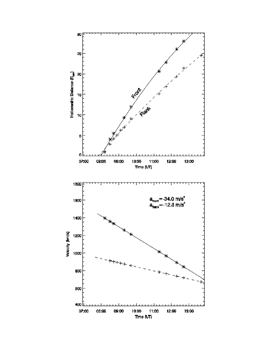
Figure 3: Upper panel: Height-time measurements at the CME front (stars) and flank (crosses). The lines are second-degree polynomial fits to the data. Lower panel: The derived speeds and decelerations.

We analysed the kinematics of the event by constructing height-time plots along two radial positions using the EIT, C2 and C3 images. The first position angle (PA), marked as P1 in Figure 2, corresponds to the front of the filament and consequently of the CME (PA=80^∘). The second position (P2) was taken at a random position along the southern CME flank (PA=100^∘). The position angles were measured counterclockwise from the solar North Pole. Figure 3 demonstrates that the height-time curves can be fitted well by second degree polynomials. Both curves show deceleration. The average speeds in both locations (800-1000 km/s) are well above the median speed of 476 km/s for CMEs observed with LASCO (St. Cyr et al., 2000). They are comparable to shock speeds deduced from metric type-II bursts (e.g., Klassen et al., 2000) and are similar to the measured speeds for the July 6, 1980 white light shock candidate (Sime and Hundhausen, 1987). The derived speeds, therefore, are consistent with the existence of a shock. Note that, as all coronagraphic measurements, the above heights, speeds and decelerations are projected values in the plane of the sky. In this case, however, we are confident that the measured parameters are close to their true, radial values because the CME source region is very close to the solar limb and since most CMEs appear to move radially (Hundhausen, Burkepile & St. Cyr, 1994; St. Cyr et al., 1999, 2000) the jet-CME was most likely propagating close to the plane of the sky.

We measured the mass across the sharp feature and derived the corresponding density profile, as follows: First, the LASCO C2 and C3 images were corrected for vignetting, exposure time and other instrumental effects and were calibrated in units of excess brightness after subtracting a pre-event image. This is a standard procedure for the analysis of coronagraph CME observations (Poland et al., 1981) and, for the LASCO case, is described in some detail in Vourlidas et al. (2000). The resulting excess brightness images were converted to excess mass images under the usual assumptions: (i) the scattering electrons are concentrated on the plane of the sky and, (ii) the ejected material comprises a mix of completely ionized hydrogen and 10% helium. These images are shown in Figure 2. The visibility of the CME flank is enhanced somewhat by this procedure and it can be followed out to at least 20 R_☉. We measured the mass profiles across the front at the same position angle (P2) where the height-time measurements were taken. To improve the signal-to-noise ratio, especially at the larger elongations, we averaged over a 10^∘-wide swath along the flank. The result is a measurement of the line of sight density of the white light structure. To convert the profiles to volume density we made another assumption about the unknown depth of the feature along the line of sight. The sharpness of the feature suggests a limited extent along the line of sight. Therefore, we assumed its depth equal to its width ($\sim 0.2$ R_☉), as measured in the C2 image at 8.30 UT. The resulting profiles represent estimates of excess density. We converted them to total density profiles by adding the pre-event (background) coronal density. This density was derived from the closest C2 polarization brightness (pB) image using the well-known pB inversion method (van de Hulst, 1950; Hayes, Vourlidas & Howard, 2001). The pB image was obtained at 21:00 UT on April 1, before the passage of the earlier CME discussed in the previous section. It is likely that the derived background density might be slightly higher than the actual density at the time of our event. The final density profiles are shown in Figure 4 where they are compared to the commonly-used SPM background model (Saito, Poland & Munro, 1977) coronal density profile. We see that the background density profile, derived from the C2 pB image, agrees very well with the SPM model profile. The density increase across the feature is very sharp in the C2 images and the profiles are very similar to the expected density profile across a shock. The profile retains its sharpness until 9:18 UT, becoming smoother at larger distances (not shown here). The density jump across the profile is about a factor 3 (at 8:30 UT) and strongly suggests that the sharp white light feature is actually a shock. However, one should note that, given the assumptions used to derive the density profiles, this density jump is only an estimate. To examine the viability of a shock at the flanks of the CME, we simulate the event using the measured speeds and background density profiles as constraints.

3.2 MHD Simulation

We start with a time-dependent, 2D plane-of-sky ideal MHD model. The model is described by the standard equations of MHD theory (e.g., Priest, 1982) with additional momentum and heating terms to accommodate the bimodal (fast, slow) solar wind (Wang et al., 1998; Wu et al., 2000). The complete set of equations is given in Wang et al. (1998). The model incorporates four constraints that are based on the LASCO observations. Namely, (i) the CME does not have a loop or a cavity preceeding its core, (ii) the CME center is located at 80^∘ counterclockwise from the solar north pole, (iii) the event shows significant deceleration and (iv) the simulated density profiles should match the observed ones (Figure 4). Finally, we are not interested in the details of the initiation of the event and thus we use a simple initiation mechanism which is described later.

To accommodate the first constraint we need to consider the initial magnetic field topology. Simulations with closed field configurations and beta ratios of the order of unity tend to lead to loop-cavity-core CME morphologies with considerable latitudinal extent while low beta, open field configurations result in elongated, laterally confined ejections (see Figure 5 and Table 1 in Steinolfson et al., 1978). Therefore, closed field configurations are better suited for modeling CMEs similar to the west limb event in Figure 1 or to the loop-like CME described in Sime and Hundhausen (1987). Instead, the narrow width of the CME and the absence of the 3-part structure, led us to the choice of a radial magnetic field (Figure 5) with beta ratios ranging from 0.83 at the equator to 0.34 at the poles. Figure 5 also shows the initial solar wind velocity and density distribution at the position angle of the CME core (P1). The model density is in good agreement with the measured density. The background flow velocity is obtained from the MHD model. Note that the contrast between the CME center and polar background flow velocities is insignificant because we use a radial magnetic field configuration. To account for the observed deceleration, we used a spatially dependent polytropic index ($\gamma=1.05$ between 1-4 R_☉, then linearly increasing to 1.45 at 30 R_☉). This implies that the energy equation for the ideal MHD model is modified to include non-adiabatic processes (Wang et al., 1998). To reduce computation time, we assumed symmetrical conditions at the angular computational boundaries at 0^∘ and 80^∘ from solar north. In other words, the CME is considered symmetric relative to its center at P1 which is consistent with the appearance of the CME in the LASCO images. The lower radial boundary is the solar surface (1 R_☉) and is prescribed according to the theory of characteristics (Wu and Wang, 1987). The initial conditions at the solar surface at locations P1 and P2 are: magnetic field 1.5 G and 1.2 G, number density $5\times 10^{7}$ cm^-3 and $10^{8}$ cm^-3, and temperature $2.24\times 10^{6}$ K and $1.74\times 10^{6}$ K, respectively. A detailed mathematical representation of the compatibility relations obtained by methods of characteristics in two dimensions is given in Suess, Wang, & Wu (1996), for example. In short, we specify that $B_{r}$ and $p/\rho^{\gamma}$ are constants at the lower boundary (the solar surface), and $p$, $B_{\theta}$, $\rm{v}_{r}$ and $\rm{v}_{\theta}$ are computed from the compatibility relations (Wu and Wang, 1987; Wang, 1992; Suess, Wang, & Wu, 1996). The linear extrapolation method is used to compute the upper radial computational boundary at 30 R_☉ which has non-reflecting boundary conditions. The system is in quasi-steady equilibrium in its initial state. The same modeling method was applied in the simulation of another event in Wu et al. (1999).

The sole objective of our simulation is the identification of the nature of the flanks of this particular jet-CME, not the processes of CME initiation. Thus, we do not seek elaborate initiation configurations that attempt to model CMEs in more realistic ways but impose a premium on computational time. Instead, we initiate the event with a simple pressure pulse. In any case, the nature of the CME flanks should not depend on the details of its initiation mechanism. We introduce a 20^∘-wide pressure perturbation by raising the density but keeping the temperature identical to the local value at the solar surface, which is symmetric relative to the center of the event (P1). This density pulse is three times higher than the background and the maximum perturbed velocity at its center reaches 200 km/s at 200 seconds, maintains this value for about 5000 seconds, and then declines to the background velocity. This perturbation represents a mass flow that forms as an ejecta to produce the observed shock. The total computational time is 293 minutes.

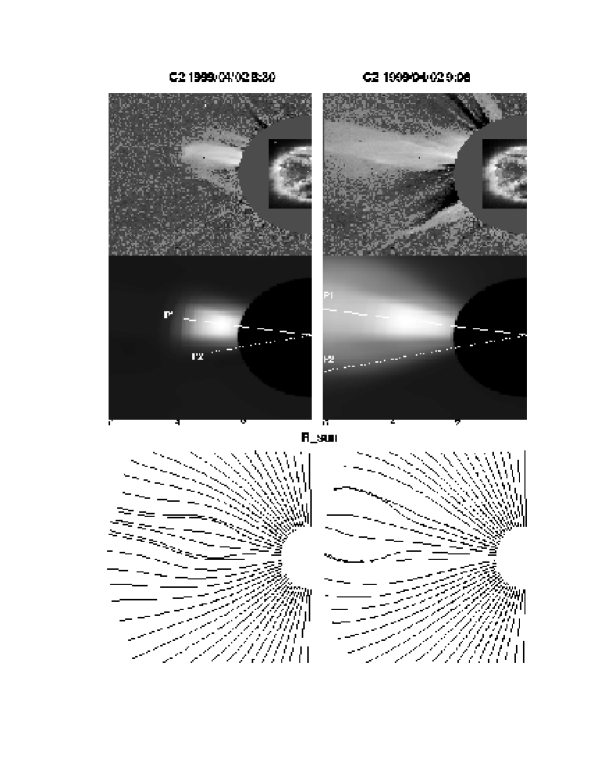
Figure 7: Comparison between the C2 observations (top panels) and the simulated pB images (middle panels) computed from our CME model. The model magnetic field line configuration is also shown (bottom panels).

Figure 4 demonstrates the excellent agreement between the simulated and measured density profiles. The simulated and measured height-time curves are compared in Figure 6. Overall the simulation reproduces the CME measurements well. We are also interested in reproducing the morphology of the event. In Figure 7, we assemble the observed images together with simulated pB images and the magnetic field configuration. The core of the CME is immediately recognized acting as the piston for the bow-shock feature. We see that the choice of radial field led our model to a good match of the narrow width of the CME.

3.2.1 Analysis of Simulation Results

The next step is the analysis of the waves produced in the simulation. In an MHD medium, the information from a disturbance can propagate with one of two characteristic speeds; the slow-mode, $V_{s}$ or the fast-mode, $V_{f}$ speed that are given by

$$V_{f,s}^{2}=0.5\left[(V_{\alpha}^{2}+C_{s}^{2})\pm\sqrt{(V_{\alpha}^{2}+C_{s}^{2})^{2}-4V_{\alpha}^{2}C_{s}^{2}\cos^{2}\theta}\right]$$ (1)

where $V_{\alpha}$ is the Alfvén speed ($V_{\alpha}=B/\sqrt{4\pi\rho}$), $C_{s}$ is the sound speed ($C_{s}=(\gamma p/\rho)^{1/2}$), and $\theta$ is the angle between the magnetic field and the direction of the wave propagation. For propagation parallel to the magnetic field ($\theta=0$), we find that $V_{f}=V_{\alpha}$ and $V_{s}=C_{s}$. In the case of propagation perpendicular to the magnetic field, only the fast-mode propagates with speed $V_{f}=(V_{\alpha}^{2}+C_{s}^{2})^{1/2}$.

When the wave is compressive, it may be observed in the coronagraph images if the density increase at the wave front is large enough. For sufficiently energetic drivers, the wave may steepen into a shock. Note that all MHD shocks are compressive shocks. From shock theory (Jeffrey and Taniuti, 1964), the existence of a MHD shock solution for propagation parallel to the field requires

$$V_{f}>U_{sh}>V_{s}, \qquad\rm{slow\ MHD\ shock}$$

$$U_{sh}>V_{f}, \qquad\rm{fast\ MHD\ shock}$$ (2)

and for propagation perpendicular to the magnetic field requires

$$U_{sh}>(V_{\alpha}^{2}+C_{s}^{2})^{1/2}$$

where $U_{sh}$ is the normal component of the relative shock speed

$$U_{sh}=(\vec{V}_{prop}-\vec{V}_{SW})\cdot\vec{e}$$ (3)

where $\vec{e}$ is the normal to the shock front, $V_{prop}$ is the propagation speed of the disturbance and $V_{SW}$ is the solar wind speed. In other words, $V_{prop}$ is the usual speed derived from the coronagraph measurements and $U_{sh}$ is the speed of the disturbance in the solar wind frame. To derive the propagation speed from the simulation we follow Wu et al. (1996) and identify the locations of the shock ($r_{1},r_{2},...,r_{n}$) at times $t_{1},t_{2},...,t_{n}$. Then

$$V_{prop}={{r_{i+1}-r_{i}}\over{t_{i+1}-t_{i}}}$$ (4)

The simulation results for $U_{sh}$, $V_{f,s}$, $V_{SW}$ and $V_{prop}$ are shown in Tables 1 and 2 for both the CME flank and front, respectively. The characteristic speeds are calculated at a point in the pre-shock region. We see that the wave velocity is larger than the fast-mode speed at both locations. Therefore, our simulation supports the existence of a shock at the flanks of the CME. But could this shock be visible in the white light images? We can check the visibility of the shock by estimating the density increase across the shock front as follows. For the fast-mode shock the Mach number is defined as

$$M_{\alpha}={{U_{sh}}\over{V_{f}}}$$ (5)

The maximum density increase across the shock front occurs for propagation along the magnetic field

$${{\rho_{2}}\over{\rho_{1}}}={{(\gamma+1)M_{\alpha}^{2}}\over{(\gamma-1)M_{\alpha}^{2}+2}}$$ (6)

where $\rho_{1}$,$\rho_{2}$ are the upstream and downstream densities, respectively. For propagation at any other direction, the density compression is smaller than Eq.(6) and there is no exact formula for it. Only for very large Mach numbers, the density compression reduces to

$${{\rho_{2}}\over{\rho_{1}}}={{\gamma+1}\over{\gamma-1}}$$ (7)

for any propagation direction. From Eqs (5) and (6) we can now calculate the maximum density compression for the shock. The results are shown in Tables 1-2 for the CME flank and front, respectively. It may be noted that we use the polytropic index $\gamma$, and not the ratio of specific heats, in computing the density compression ratios. The results are close to the measured density compression, taking into account that the actual shock does not propagate along the magnetic field. The actual compression and Mach numbers should be less than the predictions in Tables 1-2.

In summary, the simulation leads us to the following conclusions:

• The observed bow shaped feature at the flank of the CME is the density enhancement from a fast mode MHD shock.

• The shock strength measured by its Mach number remained high throughout its propagation in the C2 and C3 fields of view.

• The observed and model density enhancements (Fig. 4) show very good agreement. The measured density compression ratios are slightly lower than those predicted by the shock jump condition. This is expected because the shock is propagating at an oblique angle to the largely radial magnetic field, as an inspection of the images suggests.

• The deceleration of the shock and the front is simulated by using a spatially dependent polytropic index. We do not model the energy dissipation processes that result in the deceleration; instead, we use a spatially varying polytropic index as a proxy for the energy dissipation. We have used the value of the spatially varying polytropic index at the location of the shock in computing the density compression ratio. In the absence of an explicit energy equation for the flow and knowledge about radiation losses at the shock, we feel that this is a reasonable approach. If we did solve an explicit energy equation for the flow, we would use the ratio of specific heats in order to compute the ratios of various quantities across the shock. However, this too would not be correct if the shock were lossy; one would then have to employ a separate energy balance equation across the shock that takes these losses into account.

4 Discussion

As we pointed out in the introduction, it is generally difficult to differentiate between the white light signatures of shocks (or waves) and those of coronal ejecta such as loops and filaments. For the event we examined here, we can exclude the possibility that the flanks of the CME correspond to coronal structures for several reasons.

First, there is no visible ejecta ahead of the jet-CME. The absence of overlying material might be due to an earlier, larger CME event that entered the C2 field of view at 1:30 UT. The earlier CME propagated along the same path as our event and possibly carried away some of the overlying corona. It is likely that the coronal density above the east limb was still low when the second eruption occurred.

Second, there is no evidence for preexisting or erupted large coronal loops (on scales comparable to the white light front) in the observations of every available wavelength, from EUV to X-rays.

Third, the flanks of the CME diffused rapidly as they propagated outwards. This behaviour is inconsistent with that of a coronal structure. This is readily apparent from a comparison to the filamentary structures in the CME core that remain identifiable at large heliocentric distances.

Fourth, the southeastern streamer is clearly deflected when the CME flank reaches its location. We then see the deflection propagating to the adjacent streamers thus creating a ”front” traveling southwards with a slower speed than the CME front or its flanks (Figures 1-2). This behavior is expected from a shock on theoretical grounds (Odstrc̆il and Karlický, 2000; Van der Holst, Van Driel-Gesztelyi & Poedts, 2002). It is, also, quite common in LASCO CME images where it has been interpreted as an indirect signature of shock or waves caused by high-speed CMEs (Sheeley, Hakala & Wang, 2000).

From the above arguments, we deduce that the sharp white light feature at the flank of the CME is likely a wave. Whether it is actually a shock or not depends on the local coronal conditions. However, no direct measurements of the magnetic field or the coronal density exist. Thus we employed a simulation (§3.2) to assess the likelihood of a shock. As the high CME speeds suggest and the results of the simulation support, the CME flank is likely the signature of a fast mode MHD shock. The lack of metric type-II emission does not contradict our conclusion since metric type-II bursts do not always accompany fast CMEs and vice versa (e.g., Cliver, Webb & Howard, 1999; Gopalswamy et al., 2000).

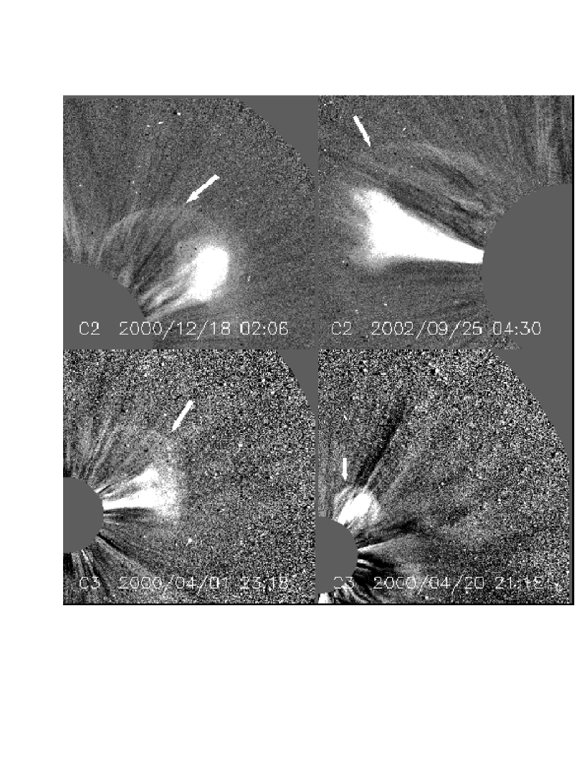
Figure 8: Examples of candidate white light shock signatures in LASCO CME observations. The LASCO telescope and the time of the event are shown on the figure. The arrows indicate the white light structure that could be the density enhancement from a shock. A preevent image has been subtracted from all images.

To our knowledge, this event is the best case for a direct identification of a white light shock in a coronagraph image. It doubles the number of CME shock candidates to date (Sime and Hundhausen, 1987, this work). Clearly, this is a very small sample and does not permit any conclusive arguments on whether the CME fronts or other CME features seen in LASCO images are indeed shocks. It is important to extend this work with further studies. There are many fast LASCO CMEs that exhibit sharp features, along either their fronts or their flanks (Fig. 8). Based on the present work, it is likely that these features could be shock or fast mode wave signatures. This information might be proven useful in the analysis of these events by providing, for example, the possible locations of type-II sources.

Another important result, in our opinion, is the simultaneous observation of a streamer deflection and the shock wave responsible for it. Although, streamer deflections have always been interpreted as the indirect signature of a CME-associated disturbance, the “hard” evidence was missing, until now. It is apparent, that the disturbance propagates through the streamer at a lower speed than in the open corona. This is most likely due to the high streamer density but projection effects may come into play (Sheeley, Hakala & Wang, 2000) and would probably complicate the derivation of any physical parameters about the streamer (or the wave). Although it could yield interesting results on the properties of shocks and streamers, no such analysis has been carried out so far, to our knowledge.

Another noteworthy consideration is the scale of the event. We showed that apparently small spray-like ejections in the low corona can give rise to a CME with significant influence over a much larger area. Yet, the brightest part of the CME (its massive core) is constrained within a narrow width ($<20^{\circ}$). If this was an earth-directed event, it would have remained inside the coronagraph occulters and hence would not have been detected. These arguments raise the question whether there exists a class of undetected earth-directed CMEs that can have some influence on the terrestrial space weather conditions. This question cannot be answered until observations of CMEs along the sun-earth line become available during the planned STEREO mission.

5 Conclusions

We have analysed a unique CME which exhibited a sharp feature at its flanks reminiscent of shock signature. From the analysis of the LASCO data and other available observations, we concluded that the white light flanks could not be coronal structures. We employed a MHD simulation to assess the possibility of the flanks being the density enhancement from a shock. We used the measured speeds and coronal densities as constraints to the simulation and showed that a fast MHD shock was formed at the front and the flank of the CME. We conclude that shocks could be directly observed in white light coronagraph images, under suitable conditions.

The event also provided us with the first direct observation of a streamer deflection by a fast mode shock, thus lending firm support to the interpretation of the commonly-seen streamer deflections as proxies to CME-induced coronal shocks. Although the appearance of this CME is rather unique, it is not fundamentally different that the ejections seen daily in the LASCO images. Therefore, the aforementioned results could be used in the search for shocks signatures in other events.

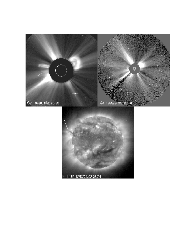
Figure 1: LASCO C2 (left), C3 (right) and EIT 195Å (bottom) images on April 2, 1999, showing the CME event in the overall context of the solar corona. The arrow in the EIT image shows ejecta that constitute the core of the white light CME. The arrows, in the C2 and C3 images, point to the shock-like feature that is analysed in the paper. The feature is more visible in the processed images in Figure 2. The circle inside each occulter marks the size of the solar disk for that coronagraph. Planet Venus is visible in the C2 southwestern quadrant.

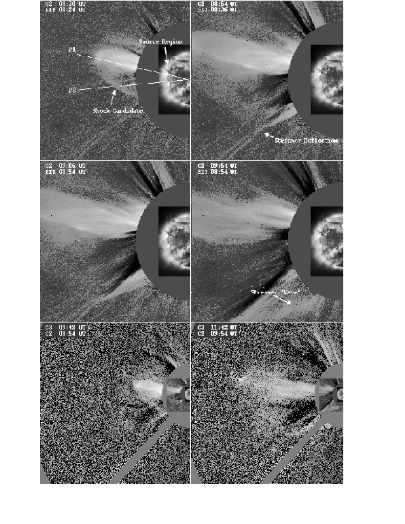
Figure 2: LASCO C2, C3 and EIT 195Å observations of the CME on April 2, 1999. Only part of the eastern field of view is shown. A pre-event image has been subtracted from the C2 and C3 images which were subsequently calibrated in units of excess mass (see § 3.1 for details). The type and time of each observation is shown at the upper left corner of each frame. The lines labeled P1 and P2 demarcate the position angles where the height-time and density measurements were made (see text). Also marked on the images are the locations of the CME source region, the shock front candidate and other features discussed in the text.

Figure 4: (a) Density profiles across the CME flank (lines with crosses) for two C2 images. The profiles are averages along a 10^∘ swath perpendicular to the flank normal at P2. The solid line is the background coronal density derived from a pre-event pB image. The dotted line is the SPM model equatorial coronal density profile. (b) The corresponding simulated density profiles. (see § 3.2 for details).

Figure 5: The initial quasi-steady state density, background flow velocity and magnetic field configuration for the simulation. The radial density distribution of the model is closely matched to the observed one. In the right panel, the solid lines represent the magnetic field lines and the dashed lines represent the solar wind velocity field. The arrows point to the direction of the magnetic field and solar wind flow, respectively.

Figure 6: Height-time and velocity profiles derived from the MHD simulation (solid lines) are compared to the LASCO data (crosses) for both the CME front and flank. The plot is similar to that of Figure 4.

Table 1: The Model-derived Velocity and Shock Data for the Flank of the CME.

Time	$V_{s}$	$V_{f}$	$U_{sh}$	$V_{sw}$	$V_{prop}$	$\gamma$	$M_{\alpha}$	$\rho_{2}/\rho_{1}$
(UT)	(km/s)	(km/s)	(km/s)	(km/s)	(km/s)
08:30	153	348	659	206	865	1.05	1.89	3.36
08:54	150	256	588	252	840	1.07	2.29	4.60
09:18	147	219	508	317	825	1.13	2.31	3.99
09:42	141	206	465	335	800	1.22	2.25	3.61
11:18	76	151	302	425	727	1.35	2.00	2.76
11:42	69	134	267	433	700	1.37	1.99	2.71

Table 2: The Model-derived Velocity and Shock Data for the Front of the CME.

Time	$V_{s}$	$V_{f}$	$U_{sh}$	$V_{sw}$	$V_{prop}$	$\gamma$	$M_{\alpha}$	$\rho_{2}/\rho_{1}$
(UT)	(km/s)	(km/s)	(km/s)	(km/s)	(km/s)
08:30	158	532	1030	220	1250	1.05	1.94	3.67
08:54	153	334	901	297	1198	1.16	2.70	4.97
09:18	145	302	801	349	1180	1.22	2.75	4.62
09:42	136	284	749	366	1115	1.27	2.64	4.20
11:18	62	172	450	430	880	1.42	2.61	3.39
11:42	46	154	402	438	840	1.44	2.58	3.31

References

- Brueckner et al. (1995) Brueckner, G. E., et al. 1995, Sol. Phys., 162, 357
- Cliver, Webb & Howard (1999) Cliver, E. W, Webb, D. F., & Howard, R. A. 1999, Sol. Phys., 187, 89
- Delaboudiniére et al. (1995) Delaboudieniére, J.-P. et al. 1995, Sol. Phys., 162, 291
- Dobrzycka et al. (2003) Dobrzycka, D., et al. 2003, ApJ, 588, 586
- Domingo, Fleck & Poland (1995) Domingo, V., Fleck, B., & Poland, A. I. 1995, Sol. Phys.., 162, 1
- Gilbert et al. (2001) Gilbert, H. R., et al. 2001, ApJ, 550, 1093
- Gopalswamy et al. (2000) Gopalswamy, N. et al., 2000, Geophys. Res. Lett., 27, 1427
- Gosling et al. (1974) Gosling, J. T., et al. 1974, J. Geophys. Res., 79, 4581
- Handy et al. (1999) Handy, B. N., et al. 1999, Sol. Phys., 187, 229
- Hartle and Barnes (1970) Hartle, R. E., & Barnes, A. 1970, J. Geophys. Res., 75, 6915
- Hayes, Vourlidas & Howard (2001) Hayes, A. P., Vourlidas, A., & Howard, R. A. 2001, ApJ, 548, 1081
- Hundhausen, Holzer & Low (1987) Hundhausen, A. J., Holzer, T. E., & Low, B. C. 1987, J. Geophys. Res., 92, 11173
- Hundhausen (1988) Hundhausen, A. J., 1988, in Proc. of the 6th Solar Wind Conf., NCAR/TN-306+Proc, p. 181
- Hundhausen, Burkepile & St. Cyr (1994) Hundhausen, A. J., Burkepile, J. T., & St. Cyr, O. C. 1994, J. Geophys. Res., 99, 6543
- Jeffrey and Taniuti (1964) Jeffrey, A., & Taniuti, T. 1964, Non-linear wave propagation with application to physics and magnetohydrodynamics, Chapter 4, (Academic Press Inc: New York)
- Klassen et al. (2000) Klassen, A., et al. 2000, å, 141, 357
- Kohl et al. (1995) Kohl, J. L., et al. 1995, Sol. Phys., 162, 316
- Maia et al. (2000) Maia, D., et al. 2000, ApJ, 528, L49
- Mann et al. (1999) Mann, G., et al., 1999, Proc. of SOHO-8 Workshop, Wilson, A. (ed),ESA SP-446, p. 477
- Maxwell and Dryer (1981) Maxwell, A., & Dryer, M. 1981, Sol. Phys., 73, 313
- MacQueen et al. (1980) MacQueen, R. M., et al. 1980, Sol. Phys., 65, 91
- MacQueen and Fisher (1983) MacQueen, R. M., & Fisher, R. 1983, Sol. Phys., 89
- Michels et al. (1984) Michels, D. J., et al. 1984, Adv. Space Res., 4(7), 311
- Odstrc̆il and Karlický (2000) Odstrc̆il, D., & Karlický, M. 2000, å, 359, 766
- Poland et al. (1981) Poland, A. I., et al. 1981, Sol. Phys., 69, 169
- Priest (1982) Priest, E. R. 1982, Solar Magnetohydrodynamics, 73 pp., (D. Reidel Publ. Comp: London)
- Saito, Poland & Munro (1977) Saito, K., Poland, A. I., & Munro, R. H. 1977, Sol. Phys., 55, 121
- Sheeley, Hakala & Wang (2000) Sheeley, N. R., Hakala, W. N., & Wang, Y.-M. 2000, J. Geophys. Res., 105, 5081
- Sime, MacQueen & Hundhausen (1984) Sime, D. G., MacQueen, M. R., & Hundausen, A. J. 1984, J. Geophys. Res.89, 2113
- Sime and Hundhausen (1987) Sime, D. G., & Hundausen, A. J. 1987, J. Geophys. Res., 92, 1049
- Spitzer (1962) Spitzer, L., 1962, Physics of Fully Ionized Gases, 2nd rev. ed., (John Wiley:New York)
- St. Cyr et al. (1999) St. Cyr, O.C., et al. 1999, J. Geophys. Res., 104, 12493
- St. Cyr et al. (2000) St. Cyr, O.C, et al. 2000, J. Geophys. Res., 105, 18169
- Steinolfson et al. (1978) Steinolfson, R. S., et al. 1978, ApJ, 225, 259
- Steinolfson (1985) Steinolfson, R. S. 1985, in Collisionless Shocks in the Heliosphere: Reviews of Current Research, Geophys. Monogr. Ser., vol. 35, B.T. Tsurutani and R. G. Stone (eds), (AGU:Washington, DC), p. 1
- Steinolfson (1988) Steinolfson, R. S., 1988, J. Geophys. Res., 93, 14261
- Steinolfson and Hundhausen (1990a) Steinolfson, R. S., & Hundhausen, A. J. 1990a, J. Geophys. Res., 95, 15251
- Steinolfson and Hundhausen (1990b) Steinolfson, R. S., & Hundhausen, A. J. 1990b, J. Geophys. Res., 95, 20693
- Subramanian et al. (1999) Subramanian, P., et al. 1999, J. Geophys. Res., 104, 22321
- Suess, Wang, & Wu (1996) Suess, S. T., Wang, A. H., & Wu, S. T. 1996,J. Geophys. Res., 101, 19957
- Tsuneta et al. (1991) Tsuneta, S., et al. 1991, Sol. Phys., 136, 1
- Van der Holst, Van Driel-Gesztelyi & Poedts (2002) Van der Holst, B., Van Driel-Gesztelyi, L, & Poedts, S. 2002, in Proc. of the 10th Europ. Sol. Phys. Meeting., Wilson, A (ed), ESA SP-506, p.71
- van de Hulst (1950) van de Hulst, H. C. 1950, Bull. Astron. Inst. Netherlands, 11, 135
- Vourlidas et al. (2000) Vourlidas, A., et al. 2000, ApJ, 534, 456
- Wang (1992) Wang, A. H. 1992, Ph.D. dissertation, Univ. of Alabama in Huntsville.
- Wang et al. (1998) Wang, A. H., et al. 1998,J. Geophys. Res., 103, 1913
- Wu et al. (1996) Wu, C. C., et al. 1996, Sol. Phys., 165, 377
- Wu and Wang (1987) Wu, S. T., & Wang, J. F. 1987,Comput. Meth. Appl. Mech. Eng., 64, 267 J. Feynman (eds), (AGU:Washington, DC), p. 83
- Wu et al. (1999) Wu, S. T., et al. 1999, J. Geophys. Res., 104, 14789
- Wu et al. (2000) Wu, S. T., et al. 2000, ApJ, 545, 1101