Correlations between the WMAP and MAXIMA Cosmic Microwave Background anisotropy maps

Abstract

We cross-correlate the cosmic microwave background temperature anisotropy maps from the WMAP, MAXIMA-I, and MAXIMA-II experiments. We use the cross-spectrum, which is the spherical harmonic transform of the angular two-point correlation function, to quantify the correlation as a function of angular scale. We find that the three possible pairs of cross-spectra are in close agreement with each other and with the power spectra of the individual maps. The probability that there is no correlation between the maps is smaller than $1\times 10^{-8}$. We also calculate power spectra for maps made of differences between pairs of maps, and show that they are consistent with no signal. The results conclusively show that the three experiments not only display the same statistical properties of the CMB anisotropy, but also detect the same features wherever the observed sky areas overlap. We conclude that the contribution of systematic errors to these maps is negligible and that MAXIMA and WMAP have accurately mapped the cosmic microwave background anisotropy.

1. Introduction

Temperature fluctuations in the cosmic microwave background (CMB) encode a vast amount of cosmological information about our universe. CMB photons released from the primordial plasma at the time of recombination approximately 380,000 years after the Big Bang, provide thus a picture of the universe in its infancy only somewhat modified by low-redshift effects such as reionization. Recently WMAP produced a 13^′ full sky measurement of the CMB temperature anisotropy (Bennett et al., 2003a). This map has been used in conjunction with other CMB and cosmological data to constrain a number of cosmological parameters to unprecedented accuracy (Spergel et al., 2003). Previous to WMAP a number of experiments produced high quality maps of CMB temperature anisotropy. These included both balloon borne bolometric experiments such as BOOMERANG (de Bernardis et al., 2000; ruhl/etal:2002, Ruhl et al.(2002), MAXIMA-I (Hanany et al., 2000; Lee et al., 2001), and ARCHEOPS (Benoit et al., 2003), and ground based interferometric experiments, CBI (Padin et al., 2001; Mason et al., 2003), DASI (Halverson et al., 2002), and VSA (Grainge et al., 2002). Tight constraints were placed on cosmological parameters from these experiments as well (e.g. Jaffe et al. (2001); Netterfield et al. (2002); Stompor et al. (2001); Abroe et al. (2002); Pryke et al. (2002)).

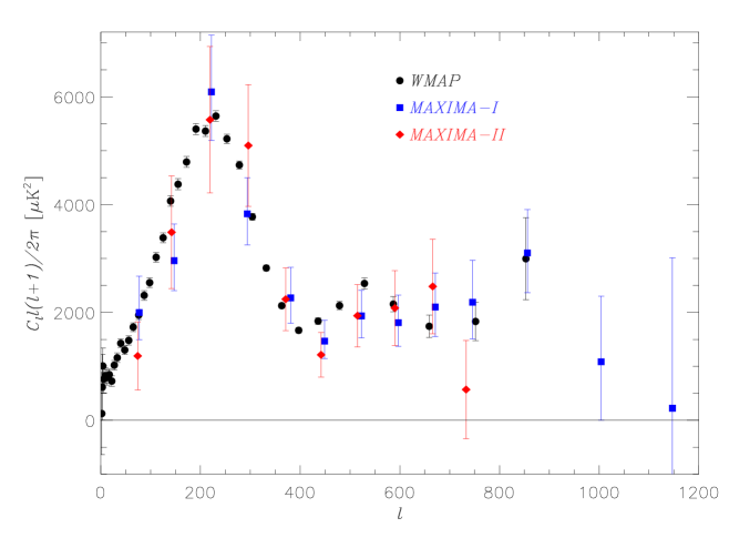
Given the longer observations and higher sensitivities of recent CMB experiments the theoretical analysis is more likely to be limited by systematic rather than statistical errors. It is therefore important to ensure that systematic errors in these experiments are sub-dominant compared to statistical errors. A comparison of the power spectra from the experiments can provide some confidence that systematic errors are not dominant. For instance the power spectra of WMAP, MAXIMA-I, and MAXIMA-II are shown in Figure 1. Note that no calibration adjustments have been made to the data. For experiments which observe overlapping parts of the sky the close agreement of the power spectra does not necessarily imply that the spatial fluctuations detected by the experiments are identical. In such cases, and particularly when the experiments have similar angular resolution, a more stringent test for systematic errors is to cross correlate the temperature fluctuations of one map with the fluctuations in the other. Positive correlations between temperature anisotropy maps would also enhance the confidence in the reconstruction of the spatial pattern of the CMB. Some difficulties arise if the two experiments under consideration have different pixel resolutions and beam profiles, which is usually the case. In that case a straightforward pixel to pixel comparison is no longer accurate because the CMB signal contained in corresponding pixels is not the same, and a more elaborate technique needs to be employed.

Figure 1.— The CMB angular power spectra as measured by WMAP (Hinshaw et al. (2003), black circles), MAXIMA-I (Lee et al. (2001), blue squares), and MAXIMA-II (red diamonds). No adjustments have been made to the calibration for any of the spectra. For the analysis in this paper we use the version of the MAXIMA -1 data published by Hanany et al. (2000) (see Section 3).

In this paper we use the cross-spectrum as a technique to cross-correlate the maps of WMAP and MAXIMA. This is the first reported cross-correlation of a CMB map with the map of WMAP, and the first release of data from the MAXIMA-II flight.

Other comparisons of CMB anisotropy maps from different experiments have been performed in the past (e.g. Ganga et al. (1993), Tenerife and DMR (Linweaver et al., 1995), MSAM and Saskatoon (Knox et al., 1998), and QMAP and Saskatoon (Xu, Tegmark, & de Oliveira-Costa, 2002)). However, none of these analyses used the cross spectrum as a technique for quantifying the amount correlation between data sets.

This paper is organized as follows: in Section 2 we give details of the cross spectrum and its use for quantifying the amount of correlations between two CMB anisotropy maps at various angular scales. In Section 3 we discuss the maps used in our analysis. Results of the calculation of the power and cross-spectra for the maps, and an analysis of the difference maps are given in Section 4. We discuss the results in Section 5, and summarize in Section 6.

2. Method

Perhaps the simplest way to compare quantitatively two maps is to calculate a $\chi^{2}$ for their difference. This statistic has the limiting feature that only overlapping sections of the maps can be included, and the maps must have identical pixelizations. Additionally, if the maps have different beam window functions, then the signal in corresponding pixels is different and the distribution of the $\chi^{2}$ statistic would no longer be $\chi^{2}$ distributed. The statistical interpretation of the $\chi^{2}$ value would therefore be difficult.

There are a number of statistics which can be calculated between two CMB maps to quantify their consistency, e.g. the linear and rank correlation coefficients (Press et al., 1992). Unfortunately, these correlation coefficients also suffer from the same difficulties as the $\chi^{2}$ statistic.

Several authors derived statistics which do take into account partial overlapping maps, different pixelizations and beam profiles. Knox et al. (1998) derive both Bayesian and frequentist techniques for correlating CMB maps, and apply these statistics to data from the MSAM92, MSAM94, and Saskatoon experiments. They advocate the calculation of the “contamination parameter”, which gives the probability distribution for the magnitude of a signal that is not common between the two data sets under consideration. A low value for the contamination parameter implies that the data sets are consistent. Tegmark (1999) defines a “null-buster” statistic which gives the number of $\sigma$ between the difference of two maps and a hypothesis of pure noise. These statistics can be used both as an internal consistency check between detectors for the same experiment (Stompor et al., 2003) and to compare maps from different experiments.

In this paper we use the cross-spectrum to quantify the level of correlations between the data of WMAP and MAXIMA . The cross-spectrum is the spherical harmonic transform of the real space correlation function for the two maps. Whereas other statistics condense the information about correlations into a single number, and therefore result in some loss of information, the cross-spectrum retains more information by analyzing the correlations as a function of angular scale.

We now discuss the method for estimating the cross-spectrum from CMB temperature anisotropy maps. Consider two maps of the CMB called $T^{\bf(1)}$ and $T^{\bf(2)}$, respectively. Then

$$\Delta T^{\bf(1)}_{i} = s^{\bf(1)}_{i}+n^{\bf(1)}_{i}$$ (1)

$$\Delta T^{\bf(2)}_{i} = s^{\bf(2)}_{i}+n^{\bf(2)}_{i},$$ (2)

where $i$ is a pixel index, $s^{\bf(1)}_{i}$ and $s^{\bf(2)}_{i}$ are the CMB signal in pixel $i$, and $n_{i}^{\bf(1)}$ and $n_{i}^{\bf(2)}$ are the pixel noise for the first and second map, respectively. Let the number of pixels in the first and second maps be $N_{\rm p}^{\bf(1)}$ and $N_{\rm p}^{\bf(2)}$, respectively. We write the data vector in pixel space as

$$d = \left[\begin{tabular}[]{c}$\Delta T^{\bf(1)}$\\ $\Delta T^{\bf(2)}$\\ \end{tabular}\right],$$ (5)

where $d$ is now a column vector of length $N_{\rm p}^{\bf(1)}+N_{\rm p}^{\bf(2)}$. Assuming the signal and noise within each experiment are uncorrelated and that the noise between experiments is uncorrelated, and using Equations 1 and 2 we find that

$$\langle dd^{T}\rangle = M\equiv\left[\begin{tabular}[]{ccc}$S^{\bf(1)}+{\cal N}^{{\bf(1)}}$&$S^{\bf(C)}$\\ $S^{{\bf(C)}T}$&$S^{\bf(2)}+{\cal N}^{\bf(2)}$\\ \end{tabular}\right],$$ (8)

where ${\cal N}^{\bf(1)}=\langle n^{{\bf(1)}}n^{{\bf(1)}T}\rangle$ and ${\cal N}^{\bf(2)}=\langle n^{{\bf(2)}}n^{{\bf(2)}T}\rangle$ are the pixel noise covariance matrices for the first and second experiment, respectively. The quantities $S^{\bf(1)}$, $S^{\bf(2)}$, and $S^{\bf(C)}$ are the CMB signal covariance matrices, which can be written as

$$S^{\bf(1)}_{ij} = \sum_{\ell}{{2\ell+1}\over{4\pi}}C_{\ell}^{\bf(1)}B_{\ell}^{{\bf(1)}2}P_{\ell}(\cos\theta_{ij})$$ (9)

$$S^{\bf(2)}_{ij} = \sum_{\ell}{{2\ell+1}\over{4\pi}}C_{\ell}^{\bf(2)}B_{\ell}^{{\bf(2)}2}P_{\ell}(\cos\theta_{ij})$$ (10)

$$S^{\bf(C)}_{ij} = \sum_{\ell}{{2\ell+1}\over{4\pi}}C_{\ell}^{\bf(C)}B_{\ell}^{\bf(1)}B_{\ell}^{\bf(2)}P_{\ell}(\cos\theta_{ij}),$$ (11)

where $B_{\ell}^{\bf(1)}$ and $B_{\ell}^{\bf(2)}$ are the beam profiles for the first and second experiment, $P_{\ell}$ are Legendre polynomials, and $\theta_{ij}$ is the angle between pixels $i$ and $j$. The auto-spectra $C_{\ell}^{\bf(1)}$ and $C_{\ell}^{\bf(2)}$ are commonly called the power spectra for the first and second map, respectively, and $C_{\ell}^{\bf(C)}$ is defined as the cross-spectrum. In the zero noise case the cross-spectrum is limited by the requirement that $C_{\ell}^{{\bf(C)}}\leq\sqrt{C_{\ell}^{\bf(1)}C_{\ell}^{\bf(2)}}$. Otherwise $M$ would have negative eigenvalues and therefore be unphysical. Up to an irrelevant additive constant, the likelihood for $d$ is

$$-2\ln{\cal{L}} = (N_{p}^{\bf(1)}+N_{p}^{\bf(2)})\ln|M|+d^{T}M^{-1}d.$$ (12)

We maximize the likelihood $\cal L$ as a function of the two auto-spectra and the cross-spectrum. If two CMB maps have a high degree of correlation, then we expect the cross-spectrum to resemble the auto-spectra of both maps. If the signal in the two maps is not correlated the cross-spectrum should be consistent with zero at all angular scales.

To maximize $\cal L$ we adopt a Newton-Raphson technique for finding the zero of the first derivative of the log likelihood function. We use a technique similar to the one described by Bond, Jaffe, & Knox (1998) except that we use the full curvature matrix instead of the Fisher matrix when calculating the steps for convergence of the Newton-Raphson algorithm (Hobson & Maisinger, 2002). We found that use of the Fisher matrix gave non-positive definite pixel-correlation, presumably because the likelihood function of the three spectra together has a complicated structure.

The cross-spectrum method involves estimating all three power spectra simultaneously and gives rise to correlations between the different spectra. Therefore an auto-spectrum estimated for any one experiment alone may differ from the auto-spectrum calculated when estimating the cross spectrum. For the case of a full sky coverage one can show that the level of correlations between the spectra is proportional to the amplitude of the cross-spectrum, that is to the amount of common sky signal (Kamionkowski et al., 1996). We therefore expect a high level of correlations between the spectra if they share the same sky signal at low $\ell$’s where the contribution of instrument noise is smaller compared to sample variance.

Figure 2.— The beam filter functions for MAXIMA-I (dotted line), MAXIMA-II (dashed line), and WMAP (solid line) considered in this analysis. The horizontal axis is spherical harmonic multipole as a function of $\ell$.

The cross-spectrum is a powerful technique for comparing two CMB anisotropy maps because it accounts for different beam shapes, pixel resolutions and sky coverage in a simple and straightforward way. For example, one can compute the cross-spectrum for two maps that do not overlap at all. In such a case the results would not be sensitive to correlations on small angular scales. Also, though our formalism describes estimating the cross-spectrum for two maps, a further generalization could be made to estimating correlations between three or more maps simultaneously. However, given numerical subtleties which are subsequently discussed in Section 5.2, we found it prudent, while equally convincing, to estimate the correlations for only pairs of maps.

The power spectra estimated from the WMAP maps are actually the cross-spectra from different detectors from the same frequency band (Hinshaw et al., 2003). Our approach is distinct from the one used by the WMAP team in that they use a frequentist approach (Hivon et al., 2002) to estimate the cross-spectra between various detectors of the same frequency band independently from the auto-spectra. The approach we use in this paper is entirely Bayesian.

Figure 3.— A comparison of the overlap region of the MAXIMA-I (upper right panel) and the WMAP 93 GHz (upper left panel) CMB temperature anisotropy maps, and their difference map (lower panel). The maps have been Wiener filtered for a visual comparison; the non-filtered versions are used in the analysis. All modes with $\ell\leq 35$ have been removed from these maps. The MAXIMA-I map, which originally had a resolution of 10^′, has been smoothed to the WMAP resolution. The color scale is from $-250$ to $250$ $\mu{\rm K}$.

Figure 4.— The overlap sections of the MAXIMA-I and MAXIMA-II Wiener filtered maps, shown in the left and center panel, respectively. The difference of the Wiener filtered maps is shown in the right panel. The color scales range from $-300\mu$K to $300\mu$K. Note that while only the overlap section of the MAXIMA-I map is shown here, we use the entire MAXIMA-I map for all analyses.

3. The Maps

We cross-correlate CMB temperature anisotropy maps from the WMAP, MAXIMA-I and MAXIMA-II experiments. The WMAP map used is the W-band (93 GHz) foreground-cleaned map, and only the portion that overlaps with the MAXIMA-I field. By analyzing
WMAP ’s derived foreground maps we find that this portion of the W-band map is free of point sources, and contains a negligible amount of dust, free-free, and synchrotron emission. The WMAP data at 93 GHz has similar angular resolution and is closest in frequency to the MAXIMA data. This map is pixelized using the HEALPix (Gorski, Hivon, & Wandelt, 1999) pixelization in Celestial coordinates with nside$=512$, and contains 7,926 pixels. An nside=512 corresponds roughly to a pixel with a width of 7^′. Following Bennett et al. (2003a) we assume that there are no noise correlations between pixels and that the beam pattern is non-Gaussian, azimuthally symmetric and has FWHM of 13.2^′. We computed the beam window function by taking the weighted average of the individual beams for each of the four detectors used to form the final W-band map. The resulting beam profile in $\ell$ space is shown in Figure 2. The Wiener filtered version of this map is shown in the left panel in Figure 3; we use the raw data in the analysis. The Wiener filtering is performed with the corresponding best fit models for each map. A more detailed discussion of the WMAP maps is given in Bennett et al. (2003a) and of algorithms used in their computations in Hinshaw et al. (2003).

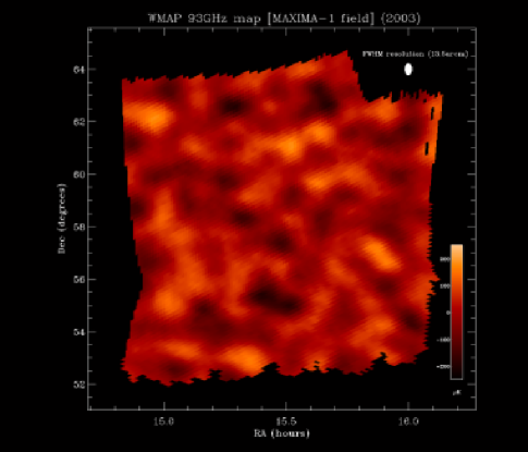
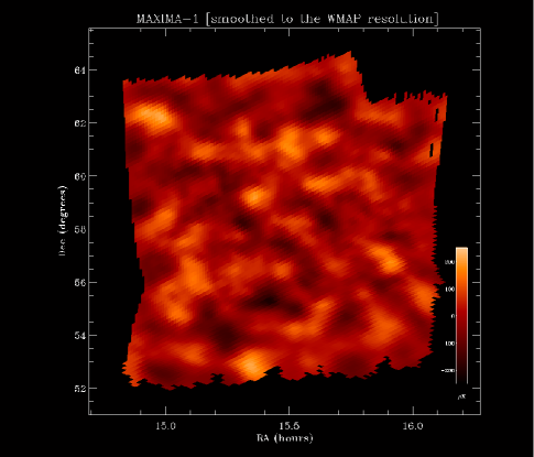
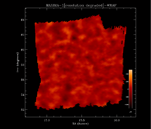
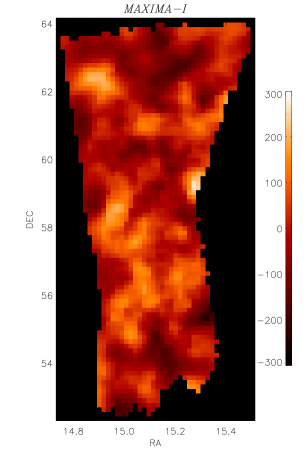
The MAXIMA map-making procedure is described exhaustively in Stompor et al. (2002). The MAXIMA-I map we use in this analysis is the 8 arcminute version of the data published by Hanany et al. (2000), which covers a larger area of the sky and has a coarser resolution compared to the data published by Lee et al. (2001). There are a total of $5,972$ pixels, and this map covers $\sim 100$ ${\rm deg}^{2}$ on the sky. It is a combination of three $150$ GHz photometers and one 240 GHz photometer. The beams for each photometer have a FWHM of $\sim 10^{\prime}$ (Hanany et al., 2000) and the effective window function is calculated using the technique described in Wu et al. (2001). The MAXIMA-I map shown in Figure 3 is Wiener filtered and smoothed to a WMAP resolution. The raw version of the map is used for all quantitative analyses. Figure 3 also shows the difference of the MAXIMA-I and WMAP Wiener filtered maps. The pattern of temperature fluctuations, which is similar in both maps, disappears in the difference map.

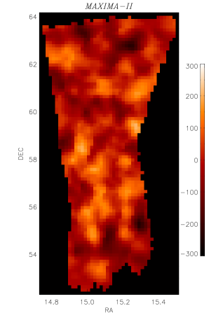
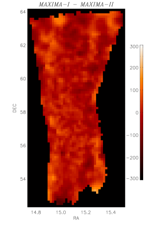
The MAXIMA-II map comes from a flight of the MAXIMA payload that took place on 1999 June 17. We use the data from four photometers at 150 GHz, and only the portion of the MAXIMA-II map that overlaps the map of MAXIMA-I. More details about the MAXIMA-II flight, data and maps are given in Rabii et al. (2003, in preparation), and Stompor et al. (2003). The MAXIMA-II map is pixelized using an 8^′ square pixelization in celestial coordinates, contains 2,757 pixels, and covers $\sim$ 50 ${\rm deg}^{2}$ on the sky. The beam profile for this map is $\sim 10^{\prime}$ FWHM, and again computed using the techniques described in Wu et al. (2001). The MAXIMA-II power spectrum shown in Figure 1 has 10 bins of $\Delta\ell=75$, extending over the $\ell$ range $35\leq\ell\leq 785$. Figure 4 shows the overlap region of the MAXIMA-I and MAXIMA-II maps and the difference map. Identical temperature fluctuations that are apparent in each of the maps disappear in the difference map.

4. Results

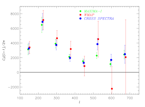
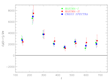
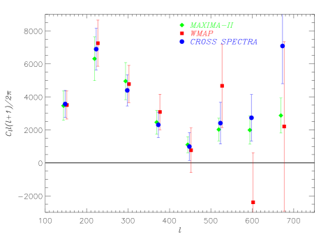
The auto- and cross-spectra for all combinations of the WMAP and MAXIMA maps are shown in Figure 5. The error bars on the spectra are the square root of the curvature of the likelihood function about the maximum likelihood parameter value. In all cases we compute the spectra in bins of width $\Delta\ell=75$, over the interval $111\leq\ell\leq 710$, and marginalize over all modes $\ell\leq 110$ and $\ell\geq 711$. The appropriate pixel window functions for each map were convolved with the beam functions in the analysis. We found that the cross-spectrum estimator did not converge when the initial bin was split in two, and this is further discussed in Section 5. In all cases the cross-spectra are consistent with the auto-spectra giving strong evidence for a correlation between the maps.

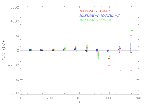
We also compute the power spectrum of the difference maps for all three pairs of maps using bins of $\Delta\ell=75$ over the range $35\leq\ell\leq 785$. The WMAP window function is used when computing the MAXIMA-I -WMAP and MAXIMA-II -WMAP difference spectra. The expected residual power resulting from different beam profiles is maximum at the bin centered at $\ell\simeq 300$, and is approximately equal to the 1$\sigma$ error bar of the MAXIMA-I /WMAP difference power spectrum. The effect is less than 1$\sigma$ for all remaining bins. We use the MAXIMA-I window function when computing the MAXIMA-I -MAXIMA-II difference spectrum. The results are shown in Figure 6. Of the 30 band power estimates for the difference maps, 28 are within 1$\sigma$ of zero power.

Table 1Cross Spectrum $\chi^{2}$ Values

Maps	DoF	$\chi^{2}_{\rm cutoff}$	$\chi^{2}$
MAXIMA-I /WMAP	8	53	191
MAXIMA-I /MAXIMA-II	8	53	241
MAXIMA-II /WMAP	8	53	150

The $\chi^{2}$ from Equation 13 calculated for all three combinations of maps. A $\chi^{2}$ greater than 53 implies that the probability that the no correlation hypothesis is true is less than $1\times 10^{-8}$.

Table 2Difference Spectrum $\chi^{2}$ Values

Maps	DoF	$\chi^{2}$
MAXIMA-I /WMAP	10	7.5
MAXIMA-I /MAXIMA-II	10	8.3
MAXIMA-II /WMAP	10	17.2

The $\chi^{2}$ of the power spectrum for the difference maps with the null spectrum.

To further quantify the level of correlation between the maps we use a $\chi^{2}$ statistic to reject the hypothesis that the maps are uncorrelated. We write our statistic as

$$\chi^{2}=\sum_{BB^{\prime}}C_{B}^{\bf(C)}F_{BB^{\prime}}C_{B^{\prime}}^{\bf(C)}$$ (13)

where the sum is over band power estimates, and $F$ is the Fisher matrix for the cross-spectrum. Because the auto-spectra and cross-spectrum are estimated simultaneously, we marginalize over the auto spectra when calculating the $\chi^{2}$.

To test the null hypothesis we choose a statistical significance $\alpha=1\times 10^{-8}$. If $\chi^{2}$ is greater than the critical value $53$, then the probability that the null hypothesis is true is less than $1\times 10^{-8}$. The results are summarized in Table 1. In all cases $\chi^{2}$ is significantly larger than the critical value giving an essential certainty that the no-correlation hypothesis is false. Note that assuming the $\chi^{2}$ of Equation 13 is $\chi^{2}$ distributed is equivalent to assuming that the $C_{B}^{\bf(C)}$ are Gaussian distributed, which is an approximation.

We also compute the $\chi^{2}$ of the difference spectra shown in Figure 6 with the null spectra to determine how consistent these are with no fluctuations in the difference maps. The results are shown in Table 2. The 10 power spectrum bins computed from the MAXIMA-I /WMAP and MAXIMA-I /MAXIMA-II difference maps have a $\chi^{2}$ of 7.5 and 8.3, respectively, with the null spectrum. The MAXIMA-II /WMAP difference map gives a $\chi^{2}$ of 17.2. There is a 7% chance of getting $\chi^{2}\geq 17.2$ for 10 DoF. Overall there is a good fit to the null spectrum model, which implies that differencing the overlap section of the maps removes the sky signal and is consistent with noise.

5. Discussion

5.1. Auto- and Cross-Spectra

The auto- and cross-spectra of the different data sets agree with each other to within $1\sigma$ over almost all $\ell$ bins giving evidence that at each angular scale all experiments are detecting the same spatial fluctuations on the sky. All auto- and cross-spectra show the first acoustic peak in the power spectrum and then a level of power that is consistent with subsequent peaks. These results are consistent with standard inflationary $\Lambda$CDM models.

Auto-spectra of the overlap section of the WMAP data give increased error bars at $\ell\geq 486$ because of the limited sky coverage of the overlap regions, and because of the beam profile of the W-band map. We find that the beam pattern alone causes the WMAP auto-spectrum error bars in the bins $\ell$=$\{\{486,560\},\{561,635\},\{636,710\}\}$ to be 2-3 larger than those for MAXIMA-I or MAXIMA-II. Negative power was found in the bin $\ell$=$\{486,560\}$ for the WMAP auto-spectra (see the top and bottom panel of  5). There is no requirement that the auto-spectrum be positive in our estimation method.

A comparison of the auto-spectra shown in Figure 5 reveals that there is a difference between band power estimates for the same dataset. This difference arises because the computation of cross-spectra involves estimating both auto- and cross-spectra simultaneously, giving rise to correlations between the different spectra. The fractional changes in power averaged over bins are 3%, 6%, and 15% for the WMAP, MAXIMA-I, and MAXIMA-II data sets, respectively. If the likelihood distribution of the band powers were strictly Gaussian, then the maximum likelihood estimates would be the same regardless of the correlations between spectra. However, the likelihood as a function of auto- and cross-spectra is somewhat non-Gaussian (see Equation 12, Bond, Jaffe, & Knox (1998)), so the correlations do effect the band power estimates. The fact that the changes between estimates are small suggests, however, that the distributions are close to Gaussian.

We note that the bin-powers are correlated at the 77% level or higher at the lowest $\ell$ bin. The correlation decreases to less than 10% at the highest $\ell$ bin for correlations between the auto-spectra and to 20% - 50% for correlations between the auto- and cross-spectra. These results are in broad agreement with expectations given the high amplitude of the cross-spectrum.

Figure 5.— The auto-spectra and cross-spectrum estimated for the MAXIMA and WMAP maps. From top to bottom: the results for MAXIMA-I /WMAP, MAXIMA-I /MAXIMA-II, and MAXIMA-II /WMAP . Note that only the portion of the WMAP map which overlaps with the MAXIMA-I field is used in the analysis.

Figure 6.— The power spectrum of the difference maps from all three data sets. The diamonds (red) are the power spectrum of the MAXIMA-I /WMAP difference map, the squares (blue) are the power spectrum of the MAXIMA-I /MAXIMA-II difference map, and the triangles (green) are the power spectrum of the MAXIMA-II /WMAP difference map. All three spectra are statistically consistent with the null spectrum.

5.2. Computational Issues

The strong correlation between the different data sets leads to some computational difficulties when attempting to find the maximum likelihood auto- and cross-power spectra. As discussed in Section 2 the cross-spectrum is limited by the requirement that $C_{\ell}^{{\bf(C)}}\leq\sqrt{C_{\ell}^{\bf(1)}C_{\ell}^{\bf(2)}}$. We find that using a quadratic estimator (Fisher matrix) method for calculating the Newton-Raphson step leads to a mis-estimate of the step for $\delta C_{\ell}^{\bf(C)}$ when starting with a guess significantly far away from the peak in likelihood space. This consequently results in a step which leads to a non-positive definite pixel covariance matrix. For example, an initial guess of a null spectrum leads to an unphysical pixel covariance matrix in all three cases we are considering. This is remedied by using the curvature matrix to compute $\delta C_{\ell}^{\bf(C)}$, as discussed in Section 2. Once the parameter values become sufficiently close to the maximum likelihood values either the curvature matrix or fisher matrix can be used to find the maximum likelihood parameters. Both techniques converge to the same set of parameters for all three analyses.

The power spectra shown in Figure 5 have been calculated with a broad initial bin at $\ell=\{2,110\}$. This is because the Newton-Raphson likelihood maximization technique did not converge if this low $\ell$ bin was split to two. Some binning structures would cause negative eigenvalues in the curvature matrix of the parameters or steps in parameter space that would lead to a non-positive definite pixel covariance matrix, both of which are unphysical.

We carried out simulations and found a similar phenomenon. The cross-spectra of uncorrelated maps or maps with a small value for the ratio of expected cross-spectrum to auto-spectrum converged to the expected answer. The calculation of the cross-spectrum also converged with simulated maps that had perfect correlation (i.e. the same map with different noise realizations) and a broad first bin with $\ell=\{2,110\}$. However it did not converge with simulated maps that had perfect correlation and two bins between $\ell$ of $2$ and $110$. Therefore, we attribute the computation problems encountered as a limitation in the method used for computing the cross-spectrum and not a feature in any of the data sets considered in this analysis.

5.3. Foregrounds and Systematic Errors

The cross spectrum and difference spectrum analyses conclusively demonstrate that all three experiments have mapped the same temperature fluctuations on the sky. However, these analyses are not sensitive to whether the shared fluctuations are CMB in origin or the result of foreground contamination or a shared systematic effect.

A careful foreground analysis was carried out by both the WMAP and MAXIMA teams. It was shown that the MAXIMA-I region of the sky at 150-240 GHz contains a negligible amount galactic contamination and that it has no detectable point sources (Hanany et al., 2000; Jaffe et al., 2003).

A detailed analysis of the foreground sources in the WMAP data is presented in Bennett et al. (2003b). Although we use WMAP ’s foreground-cleaned map,
even WMAP ’s foreground maps have negligible amount of contamination in the MAXIMA-I region. The RMS fluctuations in the WMAP 93 GHz dust, synchrotron, and free-free maps are lower than the corresponding WMAP CMB map by a factor of $17$, $42$, and $560$, respectively. Also, the WMAP team find no point sources in the MAXIMA-I region of the sky.

It is unlikely that WMAP and MAXIMA share systematic errors. We therefore conclude that the common signal in the WMAP and MAXIMA data is the cosmic microwave background radiation. Since the cross-spectra agree with the auto-spectra we conclude that within the signal-to-noise ratio of the tests systematic errors in the data are smaller compared to statistical errors.

6. Summary

We have presented a Bayesian method for estimating the cross-spectrum between two CMB temperature anisotropy maps. The method is advantageous for correlating maps because it does not require the maps to have perfect overlap, identical beam shapes or pixelizations. Using this formalism we found a high degree of correlation between the maps from MAXIMA-I, WMAP, and MAXIMA-II ; in all cases the null hypothesis is rejected with a probability higher than $1-10^{-8}$. Additionally, we computed the power spectrum of the difference maps for all combinations of the three data sets considered, and found that in each case the spectra were consistent with the null spectrum.

The results show conclusively that the temperature fluctuations detected by each of the MAXIMA-I, WMAP, and MAXIMA-II experiments are reproduced by these experiments, in overlapping regions of the sky. The close agreement of the fluctuations detected by these experiments shows that current CMB experiments are now beginning to provide us with high precision images of the true microwave sky.

References

- Abroe et al. (2002) Abroe, M. E., et al. 2002, MNRAS, 334, 11
- Bennett et al. (2003a) Bennett, C. L., et al. 2003a, ApJS, 148, 1
- Bennett et al. (2003b) Bennett, C. L., et al. 2003b, ApJS, 148, 175
- Benoit et al. (2003) Benoit, A., et al. 2002, A&A, 399, L19
- de Bernardis et al. (2000) de Bernardis, P., et al. 2002, Nature, 404, 955
- Bond, Jaffe, & Knox (1998) Bond, J. R., Jaffe, A., & Knox, L., 1998, Phys. Rev. D, 57, 2117
- Ganga et al. (1993) Ganga, K., Page, L., Cheng, E., & Meyer, S., 1993, ApJ, 509, L77
- Gorski, Hivon, & Wandelt (1999) Gorski, K. M., Hivon, E., Wandelt B. D., 1999, in Proceedings of the MPA/ESO Cosmology Conference ”Evolution of Large-Scale Structure”, eds. A.J. Banday, R.S. Sheth and L. Da Costa, PrintPartners Ipskamp, NL, pp. 37-42
- Grainge et al. (2002) Grainge, K., et al. 2002, submitted to MNRAS
- Halverson et al. (2002) Halverson, N. W., et al. 2002, ApJ, 568, 38
- Hanany et al. (2000) Hanany, S., et al. 2000, ApJ, 545, L5
- Hinshaw et al. (2003) Hinshaw, G., et al. 2003, ApJ, submitted, astro-ph/0302217
- Hinshaw et al. (2003) Hinshaw, G., et al. 2003, ApJ, submitted, astro-ph/0302222
- Hivon et al. (2002) Hivon, E., Gorski, K. M., Netterfield, C. B., Crill, B. P., Prunet, S., & Hansen, F., 2002, ApJ, 567, 2
- Jaffe et al. (2001) Jaffe, A., et al. 2001, Phys. Rev. Lett., 86, 3475
- Jaffe et al. (2003) Jaffe, A., et al. 2003, submitted to ApJ
- Kamionkowski et al. (1996) Kamionkowski, M., Kosowsky, A., & Stebbins, A., 1996, Phys. Rev. D, 55, 7368
- Knox et al. (1998) Knox L., Bond J.R., Jaffe A., Segal M., & Charbonneau D., 1998, Phys. Rev. D, 58
- Lee et al. (2001) Lee, A. T. et al. 2001, ApJ, 561, L1
- Linweaver et al. (1995) Linweaver, C. H., et al. 1995, ApJ, 448, 482
- Mason et al. (2003) Mason, B. S. et al. 2003, ApJ, 591, 540
- Hobson & Maisinger (2002) Hobson, M. P., Maisinger, K., 2002, MNRAS, 334, 569
- Netterfield et al. (2002) Netterfield, B. et al. 2001, ApJ, 571, 604
- Padin et al. (2001) Padin, S. et al. 2001, ApJ, 549, L1
- Press et al. (1992) Press, W. H., Teukolsky, S. A., Vetterling, W. T., & Flannery, B. P. 1992, Numerical Recipes in C, 2nd edn. (Cambridge, UK: Cambridge University Press)
- Pryke et al. (2002) Pryke, C., et al. 2002, ApJ, 568, 46
- (27) Ruhl, J. E., et al., preprint, astro-ph/0212229
- Spergel et al. (2003) Spergel, D. N., et al. 2003, ApJ, submitted, astro-ph/0302209
- Stompor et al. (2001) Stompor, R. et al. 2001, ApJ, 561, L7
- Stompor et al. (2002) Stompor, R. et al. 2002, Phys. Rev. D, 65, 2003
- Stompor et al. (2003) Stompor, R., et al. 2003, C.R. Acad. Sci., Paris, t.0, Serie IV, “The Cosmic Microwave Background: Present Status and Cosmological Perspectives”
- Tegmark (1999) Tegmark, M., 1999, ApJ, 519, 513
- Wu et al. (2001) Wu, J.H.P. et al. 2001, ApJS, 132, 1
- Xu, Tegmark, & de Oliveira-Costa (2002) Xu, Y., Tegmark, M., & de Olivier-Costa, A., 2002, Phys. Rev. D, 65, 083002