COMPASS : An Upper Limit on CMB Polarization at an Angular Scale of $20\arcmin$

Abstract

COMPASS is an on-axis 2.6 meter telescope coupled to a correlation polarimeter operating at a wavelength of 1 cm. The entire instrument was built specifically for CMB polarization studies. We report here on observations of February 2001 - April 2001 using this system. We set an upper limit on E-mode polarized anisotropies of 33.5 $\mu\text{K}$ (95% confidence limit) in the $\ell$-range 200-600.

1 Introduction

The recent detection of acoustic peaks in the cosmic microwave background (CMB) temperature power spectrum supports the scenario that we live in a critical density universe consisting mainly of dark matter and dark energy. In this model, large-scale structures grew via gravitational instability from seeds laid down by quantum fluctuations in a period of inflation in the early universe (Hu & Dodelson, 2001). Concordance models, in which the anisotropy measurements are combined with observations of the large-scale structure in the universe and observations of distant supernovae, sharpen this picture even further.

Further clues from the early universe have recently been found in the polarization of the CMB. The polarization signal is typically divided into two types: E-modes, which arise from scalar (density) perturbations in the early universe and B-modes, which are caused by tensor (gravitational wave) perturbations. The first attempts to measure CMB polarization occurred shortly after the discovery of the CMB almost 40 years ago. With the detection of the acoustic peaks in the temperature power spectrum now fully in hand, a variety of experiments have focused on polarization measurements. The DASI experiment has recently detected the E-mode signal at angular scales of $1^{\circ}-0.2^{\circ}$(Kovac et al., 2002) at a level of $\sim 5\mu\text{K}$. DASI also detected the temperature-polarization (TE) cross-correlation signal. Both detections are consistent with predictions from ${\rm\Lambda CDM}$ models. Because the small-scale polarization signal is expected to arise from the same processes that produce the acoustic peaks in the temperature anisotropy, detection of this signal has provided reassuring confirmation of the temperature measurements and further support for the inflationary scenario. WMAP has detected the TE polarization signal on angular scales $>0.2^{\circ}$ (Kogut et al., 2003). On scales below $5^{\circ}$ the signal is consistent with that expected from the observed temperature power spectrum. But on large scales $>10^{\circ}$, excess power is detected that is consistent with reionization occurring in the redshift range $11<z_{r}<30$ with an optical depth of $\tau=0.17\pm 0.04$. Further measurements of the polarization power spectrum will improve the determination of the fundamental cosmological parameters. In particular, measurement of the B-mode signal will constrain or detect primordial gravitational waves created during inflation.

We report here a 95 % confidence upper limit at an angular scale of $\sim 0.3^{\circ}$ in the frequency range 26-36 GHz from one season of observations with the COMPASS (COsmic Microwave Polarization at Small Scales) telescope. Although this limit is about a factor of 6 above the level of the recent polarization detections at this scale, the measurements are important for understanding the effects of foreground emission. Foreground emission from galactic and extragalactic sources can cause both E- and B- mode contamination near the level of sensitivity we have achieved. In our range of observing frequencies synchrotron radiation and emission from spinning dust are expected to be the dominant foregrounds. COMPASS observes near the North Celestial Pole (NCP). While the NCP is an exceptionally convenient region of the sky to observe from the Northern Hemisphere, it is not particularly clean of potential galactic foreground radiation. The absence of any detection of foreground signal in this region is encouraging for future measurements.

This paper is organized as follows. In section 2 we describe the COMPASS instrument, in section 3 the calibration, and in section 4 the observations. Sections 5, 6, 7, and 8 explain the data selection and analysis procedures and section 9 gives the results.

2 Instrument

COMPASS uses a receiver that was originally coupled to a corrugated feed horn with a $7\arcdeg$ FWHM beam for a large angular scale CMB polarization experiment known as POLAR (Keating et al., 2003). In order to observe smaller angular scales where a larger primordial polarization signal is expected a dielectric lens was added to the POLAR optical system and this horn+lens combination was coupled to a 2.6-meter on-axis Cassegrain telescope to form COMPASS. Here we present an overview of the instrument; further instrumental details can be found in (Farese et. al., 2003) and (Farese, 2003).

2.1 Polarimeter

The COMPASS polarimeter implements state-of-the-art HEMT (High-Electron Mobility Transistor) amplifiers that operate in the 26-36 GHz frequency range (Ka band). These amplifiers are maintained at $\approx 20$ K and provide coherent amplification with a gain of $\approx 25$ dB and a noise temperature of $\approx 20$ K. To reject $1/f$ noise from the detectors and atmospheric fluctuations two HEMTs are configured as a correlation receiver with an AC phase modulation. Each HEMT amplifies one of two polarizations observed through the same horn and thus the same column of atmosphere and same location on the sky at a given time. The resultant amplified signals are mixed down to 2-12 GHz, phase-modulated at 1 kHz, multiplexed into three sub-bands, and further amplified along separate but identical IF amplifier chains. The signals are then multiplied together and the 1 kHz phase switch is demodulated. The resulting correlated time-averaged signal amplitude is proportional to one linear combination of the Stokes parameters (Q or U in the frame of the polarimeter) as determined by the parallactic angle of the observations and the orientation of the receiver axes. A second linear combination can be obtained after a $45\arcdeg$ rotation of the polarimeter about the feedhorn’s optical axis, which allows one to measure both Stokes parameters and thus obtain all information about the linear polarization. For the observations reported here no rotation was performed; solely the polarimeter’s U polarization was measured. Depending on the observation strategy the polarimeter signal will then map to some linear combination of Q and U Stokes parameters, and similarly E and B modes, on the celestial sphere.

The three sub-bands, in order of decreasing RF frequency, are termed J1, J2, and J3. The noise of each sub-band, including telescope efficiency and atmospheric absorption (but not emission) effects, was 1040, 850, and 820 ($\mu$K$\sqrt{\text{s}}$) respectively. Each of these sub-bands is demodulated with waveforms that are both in-phase and out-of-phase with the phase-modulation signal. The desired signal is obtained from each in-phase demodulation (called J1I, J2I, and J3I) in addition to a null-signal noise monitor from the out-of-phase demodulation (J1O, J2O, and J3O). Further, a power splitter prior to the multiplexing stage allows a total power detection of each linear polarization termed TP0 and TP1; this signal is used for diagnostic purposes only. Additional details regarding the polarimeter can be found in (Keating et al., 2003).

2.2 Telescope

The COMPASS optics were designed to be as free from systematic effects as possible. Oblique reflections of light off metallic surfaces induce spurious polarization. Scattering or diffraction by a metal or dielectric will also induce a polarized signal (Kildal et al., 1988). In any off-axis telescope there will be a systematic polarization for at least one Stokes parameter. In conventional on-axis systems metallic or dielectric secondary supports necessarily obstruct the optical aperture and give rise not only to an overall polarization but also an increased side-lobe level. To avoid both of these effects COMPASS uses a microwave-transparent expanded polystyrene (EPS) secondary support system. This support was designed to position and stabilize the secondary mirror to 1 mm accuracy (Farese et. al., 2003).

The secondary mirror was designed to minimize aperture blockage. The 2.6 m diameter primary mirror had a 30 cm diameter hole in its center, so the secondary was constructed with a 30 cm diameter. A hole was left in the center of the secondary to prevent re-illumination of the receiver. A polarized calibrator made of a thermal source and wire grid was placed behind this hole. The secondary mirror is designed to under-fill the primary mirror; the primary illumination edge illumination ends 7 cm from the edge of the primary with a much faster than Gaussian taper. This results in reducing ground pickup and spillover while still maintaining a small beam size.

In order to minimize the illumination at the edge of the secondary mirror using the existing microwave horn antenna and dewar it was necessary to reduce the beam size from $7\arcdeg$ FWHM to $5\arcdeg$ FWHM with a lens. The additional requirement that this lens be cooled to reduce its contribution to the system temperature necessitated that the lens be mounted close to the horn and thus be approximately the same diameter as the horn. A simple meniscus phase-correcting lens was selected which resulted in -15 dB secondary edge illumination. This design was based on the work by (Kildal et al., 1988) and has a spherical inner surface, whose radius matches that of the radius of the horn-produced Gaussian beam, and an ellipsoidal outer surface designed to give a flat phase front at the entrance surface of the lens.

To further reduce the sensitivity of COMPASS to possible systematic effects two levels of ground screens, one affixed to the telescope and the other stationary, were constructed. The screens mounted to the telescope were attached directly to the edge of the primary mirror. These provide an additional $>50$ dB of attenuation to signals from the ground, Sun, and Moon in addition to the low sidelobe level (-60 dB) of the telescope at the location of these contaminants. Observations were conducted both with and without the outer (stationary) ground screens present. Data collected with the outer groundscreens present suffered from a larger scan synchronous signal (SSS) than data taken with them absent. It is believed that the combination of telescope spillover with the oblique scattering angle off the metallic surface of the groundscreens induced a large polarized offset. This will be discussed in more detail in section 6.

COMPASS uses a standard Az-El pointing platform. The Azimuth and Elevation stages are separate units. The Azimuth table used was a refurbished and improved version of an existing table previously designed for use with CMB observations from the South Pole. The Elevation stage was designed and built for this experiment. The position of each axis was read out by a 16 bit encoder giving a resolution of $20\arcsec$. Data acquisition of all radiometer, pointing, and “house keeping” data (such as thermometry) as well as telescope control were performed with a Pentium class laptop computer and 48 channel 16-bit ADC.

2.3 Observing Site

Our observations took place at the University of Wisconsin’s Astronomy Observatory in Pine Bluff, Wisconsin (89.685$\arcdeg$ West longitude, 43.078$\arcdeg$ north latitude). The telescope was housed in a 20 m $\times$ 15 m tensioned fabric building with a wheeled, aluminum frame. This building was rolled 20 m to the South of the telescope on tracks for observations and rolled over the telescope for shelter during periods of foul weather. By moving the building rather than the telescope we were assured of the stability of the telescope and its celestial alignment.

2.4 Pointing

We initially pointed the telescope by co-aligning an optical telescope mounted on the primary mirror with the cm-wave beam pattern using a 31 GHz Gunn oscillator mounted on a radio tower 1.9 km West-by-Southwest from the telescope. The source on the radio tower was quite easily visible through this optical telescope. Because of the proximity of our observing region to the NCP several optical observations of Polaris and a number of nearby stars were made. These Polaris observations were then used to define our absolute Azimuth and Elevation offset and thus to define our observing region. Unfortunately, misalignment of the optical telescope resulted in an Azimuth and Elevation pointing error of $+0.458\arcdeg\pm 0.027\arcdeg$ and $-0.107\arcdeg\pm 0.023\arcdeg$ respectively.

This pointing offset was discovered through observations of the supernova remnant Cas A. Cas A is circumpolar from our observing location, fairly close to our observing region, and quite bright in intensity, making it useful as a pointing tool. Three observations were made throughout the season as outlined in Table 1. Through linear fits the Elevation is seen to drift at $-1.43\arcmin\pm 2.3\arcmin$ in Elevation and $10.1\arcmin\pm 6.9\arcmin$ in Azimuth per month; There is no compelling statistically significant evidence for drifts in the pointing over the given 52 day period. Thus, a fixed pointing offset was used for all files in the analysis.

Day	Obs.	Az	error	El	error
62	4	17.4$\arcmin$	6.6$\arcmin$	-5.4$\arcmin$	4.2$\arcmin$
109	2	40.8$\arcmin$	1.8$\arcmin$	-10.2$\arcmin$	2.4$\arcmin$
114	6	29.4$\arcmin$	4.3$\arcmin$	-6.0$\arcmin$	1.8$\arcmin$
Ave		37.8$\arcmin$	1.6$\arcmin$	-7.3$\arcmin$	1.4$\arcmin$
Uncert.		5.3$\arcmin$		1.8$\arcmin$

Table 1: Successful observations of Cas A were made on the days specified by the day number in the first column. “Obs.” gives the number of full, independent rasters performed at that time. The Azimuth and Elevation offsets and errors are given in arcminutes in the remaining columns. “Ave” provides the weighted average, and thus the offsets used in analysis and “Uncert.” the scatter weighted by the uncertainty of each measurement.

2.5 Beam Determination

Raster maps of the above-mentioned “tower source” were made by using an iso-Elevation raster scan. This source was essentially in the far field of the telescope, requiring only a 0.1$\arcmin$ correction to the beamwidth at infinity. The FWHM obtained by fits of a Gaussian to the Elevation and Azimuth directions for two separate days of tower source observations are 19.2$\arcmin$ $\pm$ 0.4$\arcmin$ and 20.3$\arcmin$ $\pm$ 0.5$\arcmin$ respectively. These beam maps are confirmed by scans of Tau A. A fit of these maps with Tau A deconvolved yield a FWHM for each polarization channel and each direction (Elevation and cross-Elevation) as provided in Table 2. Note that the analysis of the Tau A data requires time series filtering which may induce a larger beam size. These numbers are further confirmed by observations of Venus which is a point source in our beam and yields beams of the two total power channels of $18.5^{{}^{\prime}}\pm 1.0^{{}^{\prime}}$ and $19.6^{{}^{\prime}}\pm 0.8^{{}^{\prime}}$. In our likelihood analysis we make the approximation that the beam is axially symmetric with FWHM $20.0^{{}^{\prime}}$, an approximation which affects our result by $\leq$ 5%.

Method	Channel	Cross-Az	Elevation
Tau A	J1I (32-35)	$21.5\arcmin\pm 0.9\arcmin$	$20.2\arcmin\pm 0.9\arcmin$
Tau A	J2I (29-32)	$22.0\arcmin\pm 0.7\arcmin$	$21.5\arcmin\pm 0.9\arcmin$
Tau A	J3I (25-29)	$23.2\arcmin\pm 0.7\arcmin$	$23.2\arcmin\pm 0.9\arcmin$
Tower	TP0, TP1	$19.2\arcmin\pm 0.4\arcmin$	$20.3\arcmin\pm 0.5\arcmin$
Venus	TP0, TP1	$18.5\arcmin\pm 1.0\arcmin$	$19.6\arcmin\pm 0.8\arcmin$

Table 2: FWHM of the beam on the sky of each sub-band derived from observations of Tau A, Venus, and our “tower source”.

3 Calibration

Given our $\sim 20\arcmin$ beam and our sensitivity level, we require a source that is no more extended than several arcminutes and of $\sim 10-20$ Jy polarized power when averaged over our telescope’s beam. Tau A (the Crab Nebula) meets these requirements and is our primary calibration source.

Historically there have been many observations of the Crab Nebula at many frequencies. If all are taken at face value they are not in agreement with each other. To narrow the field we have chosen to use only observations that were within our observing band. These observations are corrected by the spectral index of Baars ($\alpha=-0.299\pm 0.009$ (Baars et al., 1977) and the observed decay rate ($-0.167\%\pm 0.015\%/$year) of Allers (Aller & Reynolds, 1985) to contemporary, 30 GHz observations. Seven measurements satisfy these criteria (see Table 3), resulting in a most likely total power flux measurement of $339\pm 11$ Jy. These figures remained quite robust to reasonable variations in the subset of data selected and assumptions about the reported data and errorbars.

Next a total of eight polarized measurements are combined to obtain a most likely estimate of the polarized fraction of Tau A as $8.1\pm 0.9$ %. For this analysis frequency has been ignored for there is no observed frequency dependence of the data.

Finally the parallactic angle, beam dilution, and atmospheric absorption of the source at the time of each observation as well as the frequency dependence of the three correlator channels must be taken into account. A Gaussian beam of $20\arcmin$ (38.4 $\mu\text{radians}^{2}$ was used. The source is observed by performing an iso-Elevation raster scan over the target region. A linear term is fit and removed from each raster scan and the residual scans combined and compared to a template of the source derived from (Hobbs & Johnston, 1969) to obtain our calibration. All of these procedures are summarized in Table 3.

Meas.	mFlux	Err.	Year	Decay	Freq.	Cor.	cFlux	Pol. %	Par.
(Reich, 2003)	304	31	’98	0.995	32	1.02	308	8.3	152
(Hobbs & Johnston, 1969)	313	50	’69	0.947	31.4	1.01	300	8.1	158
(Hobbs et al., 1968)	387	72	’68	0.945	31.4	1.01	371	xx	xx
(Kalaghan & Wulfsberg, 1967)	340	53	’67	0.943	34.9	1.05	336	12	140
(Cartwright, 2000)	355	xx	’98	0.995	31	1.01	357	7	152
(Allen & Barrett, 1967)	373	xx	’69	0.947	31.4	1.01	358	xx	xx
(Hobbs et al., 1969)	357	xx	’69	0.947	31.4	1.01	343	xx	xx
(Mayer & Hollinger, 1968)	xx	xx	xx	xx	19	xx	xx	6.6	152
(Green et al., 1975)	xx	xx	xx	xx	15	xx	xx	6.4	148
(Boland et al., 1966)	xx	xx	xx	xx	14.5	xx	xx	8.6	146
Ave.	Flux (Jy): 339 $\pm$ 11			Pol. %: 8.9 $\pm$ 0.9			Par.: 150 $\pm$ 2
Chan	Freq	Cor.	RJ-T	mK (sig)		mV (sig)		Gain (K/V)
J1	34	0.96	1.02	11.9 $\pm$ 3.5		3.6 $\pm$ 0.16		3.32 $\pm$ 0.98
J2	30.5	1.00	1.02	15.3 $\pm$ 3.2		5.2 $\pm$ 0.14		2.98 $\pm$ 0.62
J3	27.5	1.03	1.03	19.6 $\pm$ 4.0		12.4 $\pm$ 0.37		1.58 $\pm$ 0.33

Table 3: Previous measurements of Tau A near 30 GHz. In the top porting of the table “Meas.” indicates the reference for the measurement and “Ave.” indicates the most likely value given all information in this table. “mFlux” and “Err.” as measured by the indicated group are given in Jy. “Year” indicates the year of the observation and “decay” indicates the correction for temporal signal decay between the indicated observed date and our own as calculated through (Aller & Reynolds, 1985). “Freq.” and “Cor.” are the frequency of the original observation and the correction to COMPASS central frequency as per (Baars et al., 1977). “cFlux” indicates the flux that results from applying these two corrections. “Pol. %” and “Par.” are the polarized flux percentage and parallactic angle in degrees. In the second portion corrections for the individual channels are applied. “RJ-T” is the Rayleigh-Jeans to Thermodynamic units correction, “Omega” is the solid angle of the beam in radians², “mK” is the expected signal in (thermodynamic) temperature units given all the above and “mV” is the most likely amplitude of our observations.

4 Observations

Our observing strategy was designed to optimize the probability of detecting a signal under current well-motivated theories while still allowing for systematics checks and tests. We attempted to observe a circular “disk” region centered on the NCP by maintaining a constant Elevation and scanning the telescope in Azimuth. During constant-Elevation scans the thermal load from the atmosphere remains constant and reduces both gain fluctuations of the receiver and intensity-polarization coupling in the polarimeter that could cause systematic effects. Our full scan period was varied between 10 and 20 seconds to reject longer term atmospheric fluctuations while maintaining stable and reliable telescope performance.

As the sky rotates this scanned line is transformed into a cap centered on the NCP as demonstrated in Figure 1. Further, because of the sky rotation, each half sidereal day the same region of sky is observed and allows the use of difference maps as a robust test of systematic errors. Initially this “cap” was one degree in diameter in order to allow deep integration on a small patch of sky to search for systematic effects. Half way through the season this diameter was increased to $1.8\arcdeg$ to reduce sample variance. As mentioned above there was a small pointing offset so our actual scan strategy was not the one we intended. This resulted in a loss of symmetry and thus some systematic tests but acceptable noise properties. Given the relative sizes of our beam, scan region, and pointing offset from the NCP our telescope is sensitive to both E and B modes at roughly the same level.

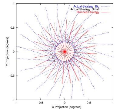
Figure 1: COMPASS scan strategy in rectangular projection about the NCP. The axes are real degrees on the sky with the positive x-axis corresponding to a Right Ascension of 0h. It is clear how constant Elevation Azimuth scans are transformed into a two dimensional map through sky rotation.

One further benefit of this scan strategy is that it simplifies the process of encoding the time stream data into a map which displays well the scan synchronous signal (SSS) while still allowing for reasonable cross-linking, sampling of a variety of parallactic angles, and systematic tests. A one-dimensional to two-dimensional map comparison allows simple identification of the SSS. If we plot the data in a coordinate system defined as Azimuth and Right Ascension it becomes quite easy to combine the data across many days and project out the modes that correspond to the SSS (see section 6).

Finally, two configurations of the ground screens were implemented; one utilizing the two layers mentioned above and one with only the inner, co-moving ground screen. These two options, combined with the two scan amplitudes mentioned above, result in a total of four “sub-seasons” of data termed SIGS, SOGS, BIGS and BOGS to specify whether the (S)mall or (B)ig scan was used and whether the (O)uter or only (I)nner ground screens were in place. Analysis was performed on each channel in each sub-season as well as combinations of channels within a sub-season, combinations of sub-seasons for a given channel, and all acceptable data.

5 Data Selection, Cleaning, and Reduction

The data analysis pipeline consists of five steps: data selection, data cleaning, intermediate Azimuth map making, full map making, and power spectrum estimation. The first three steps are outlined in this section with the last two described in greater detail in the following sections.

There were a total of 1776 hours available during our observing season which was defined as the months of March, April, and half of May of 2001. Of these, 409 had sufficiently good weather to operate the experiment. 74 hours were ignored because heavy winds disrupted the Azimuth pointing and control and 28 hours were removed because of equipment failures. This leaves a total of 309 hours of usable data observing the target region. Further cuts are made, based on the data, to select periods of stable observing conditions.

The data are divided into files of 15 minutes in length. For each file six statistics are generated: three noise-based statistics (white noise level, 1/f knee, and $\zeta$ (Keating et al., 2003) – essentially a $\frac{1}{f}$ weighted sum of the PSD); two cross correlations (between two correlator channels and between a correlator and total power channel); and a linear drift of the time stream. The 1/f knee and $\zeta$ statistics proved to be most sensitive to periods of light cloudiness or haziness. The cross correlations were most useful in identifying more rapid contaminating events such as discrete clouds, birds, or planes interfering with the observations. Finally the linear drift was used to identify dew formation on the foam cone.

A histogram of each statistic is formed and unions and intersections of files passing sets of cuts at the 3-$\sigma$ level are made. Our results were not overly sensitive to which sets were selected. The results reported here use the two cross-correlation criteria for they retained the most data while still passing all null-tests performed (see below). After all selection procedures the number of hours kept were 144, 123, and 164 for J1, J2, and J3 respectively.

Each file is then passed through a despiking procedure. Regions with excessive slopes, second derivatives, or values greater than 5 standard deviations from the mean are flagged, cut, and filled with white noise as estimated by the remainder of that file. Such flagged and white-noise filled data is not included in the data analysis. This procedure removes between 0.1 % and 32% of the data from any given sub-season. The 32% was an anomaly; it occurred only for one channel, J3, during the first sub-season where a damaged preamplifier gave rise to excessive spikes in the data intermittently. This was fixed once the cause was identified.

As a first step in the analysis, we plot the data in each fifteen minute file as a function of Azimuth. The sky rotation on this time scale is sufficiently small that a single bin of RA is needed for each file. This allows a great reduction in data size as well as a simple treatment of our most likely systematic effect (see section 6). In order to estimate the noise in these files a single data point is formed for each Azimuth bin of each Azimuth pass (i.e. leftward or rightward motion between two turn around points in the telescope motion). The standard error of the $\approx 100$ passes per file in each bin allow for an estimation of the noise to 10% and was in excellent agreement ($<$ 1% different) with the noise used in a full covariance estimation method.

6 Map Making and Scan Synchronous Signal Effects

One common systematic error in scanning style experiments is the presence of non-celestial signal that correlates highly with position in the scan, termed here “Scan Synchronous Signal” (SSS). In COMPASS such a SSS was observed and was related to a polarized offset induced by oblique reflection from the stationary ground screen or spillover to the ground. We believe that this is the result of the aggressive illumination of the secondary mirror. In all sub-seasons a variable offset and linear term (when plotted against Azimuth) are observed and removed. In the larger scan with the stationary ground screen present a quadratic signal is detected and removed as well. Once these removals are performed the residuals are consistent with Gaussian noise.

Detection of the SSS is performed easily by comparing maps made by binning data in only one dimension (i.e. Azimuth) to those made by binning in two dimensions (i.e. Azimuth and Right Ascension). If one has SSS contamination the relationship between the reduced chi-squared of the one dimensional map to that of the two dimensional map is given by

$$\chi^{2}_{1D}=1+N_{\text{bin}}\times(\chi^{2}_{2D}-1),$$ (1)

where $N_{\text{bin}}$ is the number of bins in the dimension that is collapsed and $\chi$ refers to reduced chi-squared. As shown in Table 4 there is no evidence for SSS remaining in any of the sub seasons after removal of a first order polynomial other than the Big Outer Groundscreen (BOGS) configuration.

		Two-D maps		One-D maps
Season	Channel	DOF’s	$\chi^{2}$	DOF’s	$\chi^{2}$
SIGS	J1I	244	1.00	13	0.76
SIGS	J2I	189	0.94	14	0.84
SIGS	J3I	132	1.07	13	0.73
SIGS	J1O	244	0.95	13	0.74
SIGS	J2O	189	0.95	14	0.74
SIGS	J3O	246	1.09	14	1.25
SOGS	J1I	232	1.09	13	0.45
SOGS	J2I	232	0.88	13	1.65
SOGS	J3I	240	1.00	13	1.03
SOGS	J1O	232	0.92	13	0.45
SOGS	J2O	232	1.07	13	0.84
SOGS	J3O	233	0.95	13	0.69
BIGS	J1I	182	1.08	18	0.93
BIGS	J2I	253	0.97	19	1.40
BIGS	J3I	255	0.93	19	1.20
BIGS	J1O	186	0.95	18	1.11
BIGS	J2O	180	1.24	19	1.38
BIGS	J3O	262	0.96	19	1.10
BOGS	J1I	217	1.24	19	3.96
BOGS	J2I	216	1.22	19	4.52
BOGS	J3I	212	1.17	19	4.20
BOGS	J1O	217	1.10	19	1.44
BOGS	J2O	216	1.01	19	0.68
BOGS	J3O	217	1.03	19	0.74

Table 4: The reduced Chi-squared tests for Az and RA-Az binned maps for all subseasons and channels. Note that all are consistent with no signal except BOGS J1I, J2I, and J3I which all show clear signs of unremoved Scan Synchronous Signal.

7 Map Making

As a step toward estimating the CMB polarization power spectrum we produce a map from our data. By the term “map” here we mean a pixelized representation of the data which contains information on the spatial location, most likely data value and (non-diagonal) noise correlation matrix. The nature of polarized observations requires different mapping procedures than a simple intensity map. Traditionally either a map of polarized intensity and orientation or a map of the Q and U Stokes parameters is provided. As COMPASS observed at fixed Elevation the polarization direction information (i.e. parallactic angle) is unambiguously encoded in the Right Ascension and Azimuth.

We map initially each (fifteen minute long) data file in Azimuth as described above. One useful map format in which to display the data is RA-Az coordinates. This format facilitates identification of systematic effects and spurious (or real) signals. Maps of the this style are provided in Figure 2. A second map format is a three dimensional map of RA, Dec, and parallactic angle. This second map, though sparsely populated, retains the polarization information of our observations while still providing uniformly sized pixels and is used in power spectrum estimation, though it is less intuitive to display and interpret.

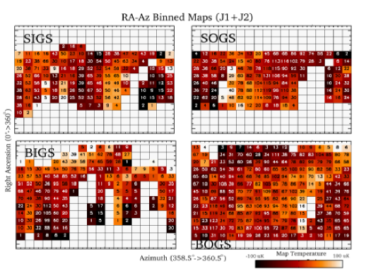
Figure 2: Maps plotted in Right Ascension and Azimuth coordinates. Shown are maps for all 4 sub-seasons of the data for J1I and J2I coadded. Color indicates intensity of the signal per pixel while the number written over that pixel is the number of Az-binned files that contribute to the value.

The noise covariance matrix is estimated from the timestream data. The off-diagonal elements of this matrix were shown to be much less than $10^{-6}$ of the amplitude of the on-diagonal elements and are therefore ignored. This is because the scan rate of $\approx 0.1$ Hz is much slower than the anti-aliasing filter knee of 40 Hz.

Given this noise matrix and the knowledge that certain modes of the map have been filtered through our polynomial subtraction method we next produce a generalized noise covariance matrix by adding to the noise matrix a constraint matrix as per (Bond et al., 1998). The constraint matrix encodes the SSS removal process and projects the removed modes out of the map by adding noise of amplitude $10^{8}$ times that of the noisiest on-diagonal element (units of $\mu K^{2}$) to the contaminated modes. These contaminated modes are constructed for each file’s Az-map and for each order of the fit removed by forming a constraint vector and taking its outer product. These constraint templates are then multiplied by the indicated noise and added to the noise covariance matrix of each file Az-map. These sub-maps are then added together in RA-Dec-parallactic angle space and a resultant generalized covariance matrix, $C_{N}$, and map of the data, $D$, are formed as given by

$$C_{N,i} = C_{n,i}+C_{c,i},$$

$$C_{N}^{-1} = \sum_{i}^{M}C_{N,i}^{-1},$$ (2)

$$\vec{D} = C_{N}\left[\sum_{i}^{M}\vec{d_{i}}C_{N,i}^{-1}.\right]$$

Subtraction of a constant term from each Azimuth file resulted in weakening of our result (i.e. increasing the uncertainty of the likelihood or 2-$\sigma$ limit) by 25%. Removing a constant term and a slope weakened it by 50%.

8 Power Spectrum Estimation

Software used to estimate the power spectrum was extensively tested using simulated maps generated from a known power spectrum. These maps were provided by the UC Davis group and used to simulate a COMPASS timeseries by the UCSB group. Several hundred realizations of this data set were produced and passed through the analysis pipeline. Both the most likely value and error estimation were proved accurate and reliable for a wide range of constraint and parallactic angle situations as shown in Table 5.

	Likelihood Probability					% Correct
Test	$-2\sigma$	$-1\sigma$	Most Likely	$+1\sigma$	$+2\sigma$	% w/i $1\sigma$	% w/i $2\sigma$
Q only	17.6	18.8	20.0	21.5	22.9	56	92
U only	16.4	17.6	19.0	20.6	22.1	68	89
Q+U	14.5	16.3	18.1	20.8	23.3	63	92
Q+10	19.6	20.3	21.1	22.0	22.8	74	94
Q+20	17.5	18.0	18.5	19.0	29.5	74	99
con0	16.8	19.3	21.9	25.8	29.5	71	86
con1	14.4	16.3	18.3	21.1	23.9	63	93
con2	16.8	19.3	21.9	25.8	29.5	71	86
recov	15.1	17.1	19.3	22.4	25.5	72	95

Table 5: Various test procedures applied to the likelihood estimator and full pipeline. The tests are described in detail in the text. The first 5 use various combinations of Q and U directly from the simulated maps. The “con” tests create sets of files of simulated Az-RA maps (our intermediate mapping) and combine them optionally adding constraints (0=none, 1=DC removed per file, 2=DC and slope removed per file). recov uses a simulated time stream generated from the simulated maps to test the full pipeline.

A flat band power model of E-mode polarization was used to generate the theory covariance matrix, $C_{T}(E)$, though use of a concordance model polarization spectrum did not significantly change our results. The likelihood of the amplitude of this flat band power is calculated using the signal to noise eigenmode method as described in (Bond et al., 1998). It is worth noting that no eigenmode in our data set has an eigenvalue greater than 1. We build the total covariance matrix $C(E)=C_{T}(E)+C_{N}$ and compute the likelihood as given by

$$L(\vec{D}|C(E))=\frac{1}{(2\pi)^{N/2}}\frac{e^{-\frac{1}{2}\vec{d}^{T}C(E)^{-1}\vec{d}}}{\left|C(E)\right|^{1/2}}.$$ (3)

This likelihood is calculated on a grid spaced uniformly in units of $\mu K^{2}$ to avoid over-biasing larger powers and is allowed to take values of negative power to test the correctness of the noise covariance matrix. This is performed under the requirement that the resultant covariance matrix remain positive definite; if the matrix becomes non-positive definite for excessively negative power that power is given a likelihood of zero as any negative power is nonphysical.

9 Results

The likelihood described above is computed for each sub-season, for the union of all sub-seasons where a slope was removed, and for the union of all data. Similarly our analysis is performed for each frequency channel independently and for the union of all channels. All results are reported in Table 6. Further, likelihood curves of the combined subseasons and channels are given in Figure 3. Five points of the integrated likelihood curve corresponding to conventional definitions for 1 and 2 standard deviations (68% and 95% confidence limits) are provided as well as the band power at which the likelihood curve obtains its maximum. This allows for a simple comparison of the various non-Gaussian curves without requiring a series of figures.

Seas	Chan	2.5%	16%	max	84%	95%
BEST	J1I	-4.600e+02	-3.800e+02	-3.700e+02	3.000e+02	1.290e+03
BEST	J2I	-1.800e+02	-2.000e+01	8.000e+01	8.400e+02	1.770e+03
BEST	J3I	-4.500e+02	-3.500e+02	-3.100e+02	3.400e+02	1.290e+03
BEST	J1O	-3.200e+02	-1.600e+02	-7.000e+01	7.600e+02	1.790e+03
BEST	J2O	-2.800e+02	-1.300e+02	-6.000e+01	8.400e+02	2.010e+03
BEST	J3O	-1.700e+02	4.000e+01	1.700e+02	1.210e+03	2.440e+03
BEST	ALL	-1.800e+02	-7.200e+01	-4.000e+00	5.000e+02	1.128e+03
ALL	J1I	-4.600e+02	-3.600e+02	-3.400e+02	4.300e+02	1.530e+03
ALL	J2I	-1.100e+02	9.000e+01	2.200e+02	1.130e+03	2.240e+03
ALL	J3I	-4.200e+02	-2.900e+02	-2.500e+02	6.100e+02	1.860e+03
ALL	J1O	-3.000e+02	-1.300e+02	-2.000e+01	8.500e+02	1.910e+03
ALL	J2O	-2.900e+02	-1.300e+02	-8.000e+01	9.600e+02	2.370e+03
ALL	J3O	-1.600e+02	7.000e+01	2.000e+02	1.360e+03	2.750e+03
ALL	ALL	-2.120e+02	-1.120e+02	-5.200e+01	4.760e+02	1.148e+03

Table 6: COMPASS results grouped by sub-season and channel. “seas” indicates sub-season: first letter is the scan size (Big or Small) and the second is the ground screen configuration (Inner or Outer Ground Screens), BEST is the union of all data represented in the sub-seasons with only a slope and DC removed. “chan” indicates the channel. The remaining columns are the values in $\mu K^{2}$ for the indicated values of the integrated likelihood curve. “max” is the peak location of the curve.

In order to explore whether or not the data were contaminated by non-cosmological signals a number of difference tests were performed. These tests are referred to as jacknife tests or difference map tests, and though not necessarily optimal they have the benefit of being both easy to implement and often easy to interpret.

Jacknife Tests
Cut used	Maps generated	Effects tested for
Left-Right	west going/east going	short time scale
	Azimuth scans	and scan effects
First-Last	first half/last half	long time scale
	of each sub-season	(e.g. thermal, etc.)
Sub Seasonal	two sub seasons	sidelobe contamination &
		long time scale
Rebinning Tests
Ra-Az	Local Sidereal Time and Az	diurnal effects
Azimuth	only Azimuth	scan synchronous

Table 7: This table describes briefly the different jacknife and binning tests that were performed and states what effect they are primarily attempting to discriminate.

Given a data vector $d_{i}$ and a noise covariance matrix $N_{i}$ for each of the $i=0,1$ maps we can form the difference map and noise covariance

$$N_{d} = \left[N_{0}+N_{1}\right],\text{and}$$ (4)

$$d_{d} = \left[d_{0}-d_{1}\right].$$ (5)

The matrices $N_{0},N_{1}$ are actually the generalized noise covariance matrices and thus include information about constraints. Therefore if a constraint is projected out of either map it is projected out of the difference map as well. Often the convention of dividing both $N_{d}$ and $d_{d}$ by 2 is implemented. Had we adopted that convention all of our difference results would be divided by 4 for they are reported in units of $\mu K^{2}$.

The tests considered are explained in Table 7 and summarized in Table 8. 66 of the indicated 68 tests were passed which is consistent with there being no spurious signals in the data at the level of several tens of $\mu$K.

Jacknife Tests
Cut used	Channels implemented	Sub-seasons Used	Total number
Day-Night	JI, JO	all	2
Left-Right	J?I, J?O	each	24
First-Last	J?I, J?O	each	24
Sub Seasonal	J?I, J?O	SIGS, SOGS, BIGS	18
Total			68

Table 8: Summary of the various combinations of channels and sub-seasons used in each jackknife test. ? means vary over each of the 3 channels. For sub-seasonal tests only those sub-seasons used in the final analysis (see section 2) were used.

10 Conclusion

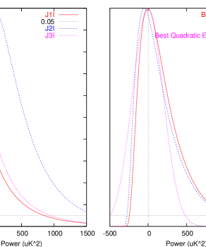
Figure 3: Likelihood curves in $\mu K^{2}$ for the E-mode flat band power for each frequency channel in the “BEST” data and for all frequencies combined for the “BEST” and “ALL” data. The quadratic estimator for the “BEST” data is included as well.

After one season of observations totaling approximate 150 hours of useful data COMPASS set a 95% confidence upper limit on polarized celestial signal of 33.5 $\mu K$ (21.8 $\mu$K 68% limit) in the $l$-range $[200-500]$. It is worth noting that a quadratic estimator approach to this analysis would have provided a limit of 22.4 $\mu K$, nearly a factor of two lower (in units of $\mu K^{2}$). This emphasizes the need for explicit calculation of a likelihood curve because the quadratic estimator is a biased estimator in low signal-to-noise situations.

It is also noteworthy that this limit is the most stringent constraint on polarized foregrounds in the NCP region on these angular scales. Because we are observing at a frequency where synchrotron emission is expected to be the dominant foreground the absence of a signal at this level bodes well for future CMB polarization experiments.

11 Acknowledgments

We thank John Carlstrom for loaning us the HEMT amplifiers used in this experiment. This research was supported by NSF grants AST-9802851 and AST-9813920 and NASA grant NAG5-11098. Brian Keating acknowledges support from the National Science Foundation’s Astronomy & Astrophysics Postdoctoral Fellowship Program. Alan Peel acknowledges support from a NASA/GSRP fellowship.

References

- Allen & Barrett (1967) Allen, R. J., & Barrett, A. H. 1967, ApJ, 149, 1
- Aller & Reynolds (1985) Aller, H. D., & Reynolds, S. P. 1985, ApJ, 293, L73
- Baars et al. (1977) Baars, J. W. M., Genzel, R., Pauliny-Toth, I. I. K., & Witzel, A. 1977, A&A, 61, 99
- Boland et al. (1966) Boland, J. W., Hollinger, J. P., Mayer, C. H., & McCullough, T. P. 1966, ApJ, 144, 437
- Bond et al. (1998) Bond, J. R., Jaffe, A. H., & Knox, L. 1998, Phys. Rev. D, 57, 2117
- Cartwright (2000) Cartwright, J: personal communication on behalf of CBI
- Farese (2003) Farese, P. C. 2003, PhD dissertation, University of California, Santa Barbara
- Farese et. al. (2003) Farese, P. C., Dall’Oglio, G, Gundersen, J. O., Klawikowski, S., Knox, L., Levy, A., Lubin, P. M., O’Dell, C. W., Peel, A., Piccirillo, L.,Ruhl, J., T. Timbie, P., 2003, To be published in ”The Cosmic Microwave Background and its Polarization”, New Astronomy Reviews, (eds. S. Hanany and K.A. Olive)
- Green et al. (1975) Green, A. J., Baker, J. R., & Landecker, T. L. 1975, A&A, 44, 187
- Hobbs et al. (1968) Hobbs, R. W., Corbett, H. H., & Santini, N. J. 1968, ApJ, 152, 43
- Hobbs et al. (1969) —. 1969, ApJ, 156, L15+
- Hobbs & Johnston (1969) Hobbs, R. W., & Johnston, K. J. 1969, Bulletin of the American Astronomical Society, 1, 244
- Hu & Dodelson (2001) Hu, W., & Dodelson, S. 2001, in Ann. Rev. Astron. Astrophys., 52