The formation history of the Galactic bulge

Abstract

The distributions of the stellar metallicities of K giant stars in several fields of the Galactic bulge, taken from the literature and probing projected Galactocentric distances of $\sim 500$ pc to $\sim 3$ kpc, are compared with a simple model of star formation and chemical evolution. Our model assumes a Schmidt law of star formation and is described by only a few parameters that control the infall and outflow of gas and the star formation efficiency. Exploring a large volume of parameter space, we find that very short infall timescales are needed ($\lower 2.15277pt\hbox{$\;\buildrel<\over{\sim}\;$}0.5$ Gyr), with durations of infall and star formation greater than $1$ Gyr being ruled out at the 90% confidence level. The metallicity distributions are compatible with an important amount of gas and metals being ejected in outflows, although a detailed quantification of the ejected gas fraction is strongly dependent on a precise determination of the absolute stellar metallities. We find a systematic difference between the samples of Ibata & Gilmore, at projected distances of $1-3$ kpc, and the sample in Baade’s window (Sadler et al.). This could be caused either by a true metallicity gradient in the bulge or by a systematic offset in the calibration of [Fe/H] between these two samples. This offset does not play an important role in the estimate of infall and formation timescales, which are mostly dependent on the width of the distributions. The recent bulge data from Zoccali et al. are also analyzed, and the subsample with subsolar metallicities still rules out infall timescales $\lower 2.15277pt\hbox{$\;\buildrel>\over{\sim}\;$}1$ Gyr at the 90% confidence level. Hence, the short timescales we derive based on the observed distribution of metallicities are robust and should be taken as stringent constraints on bulge formation models.

1 Introduction

Perhaps half of the stars in the local Universe are in bulges/spheroids (Fukugita, Hogan & Peebles 1998) and how and when bulges form and evolve are crucial clues to the origins of the Hubble Sequence. The determination of the star formation history and mass assembly history of a typical bulge would provide a stringent test of galaxy formation theories. Plausible bulge formation scenarios range from a single high-redshift dissipative ‘star-burst’ (e.g. Elmegreen 1999), through successive merger-induced lower-intensity star-bursts and stellar accretion (e.g. Kauffmann 1996), to secular models in which predominantly stellar-dynamical effects at late epochs transform the central regions of thin disks to three-dimensional bulges via bar formation and destruction (e.g. Raha et al. 1991; Norman, Sellwood & Hasan 1996). The bulge of the Milky Way is close enough that individual stars may be studied from the ground to within one scale-length of the centre; the combination of deep colour-magnitude diagrams and spectroscopically determined metallicity distributions, including elemental abundances, in principle provides both the age distribution and the chemical evolution. Here we develop a model of chemical evolution of the Galactic bulge and constrain the parameter values of our model by comparison with the available observational data.

There are several ways in which the bulge formation can be traced: a spectrophotometric analysis using multi-band broadband photometry (Peletier et al. 1999; Ellis, Abraham & Dickinson 2001) or spectral indices (Proctor, Sansom & Reid 2000) are the best approaches for unresolved stellar populations. However, studies based on integrated light lack the accuracy of analyses of the properties of individual stars, possible for our bulge. In this category one should mention the study of deep stellar colour-magnitude diagrams (Feltzing & Gilmore 2000; Zoccali et al. 2003; van Loon et al. 2003) and the distribution of stellar metallicities from spectroscopic surveys (Ibata & Gilmore 1995b; Sadler, Rich & Terndrup 1996). We know from the analyses of deep colour-magnitude diagrams (Ortolani et al. 1995; Feltzing & Gilmore 2000; Kuijken & Rich 2002; van Loon et al. 2003) that the vast bulk of the Galactic bulge is ’old’, but the use of stellar isochrones cannot tell us how old to better than $\sim 3-4$ Gyr (i.e. ages in the range $10-14$ Gyr) or tell us the dispersion of the distribution of ages to better than that. In principle, stellar elemental abundances constrain durations compared to lifetimes of the sources of the elements, but these are difficult to obtain for large numbers of stars. We demonstrate here that the shape of the overall metallicity distribution provides a complementary constraint on the duration of star formation, given an old age.

The available metallicity distributions for the Galactic bulge are reasonably well approximated by the predictions of the simple closed-box model (e.g. Rich 1990; Zoccalli et al. 2003). In many applications of this model it is a virtue that the predicted distribution is independent of the star formation rate, but this of course precludes conclusions about the star formation history being made by comparison of model predictions with observations. We have thus developed a model that is analytically simple, but retains explicitly the timescales of gas flows and star formation. Our approach makes use of the metallicity distributions of K giant stars in the Galactic bulge. We explore a single-zone model in which no a priori assumptions are made regarding the parameters that describe the infall and outflow of gas. This phenomenological “backwards” approach has proven to give valuable insight on the star formation history of early-type (Ferreras & Silk 2000a, 2000b) as well as late-type galaxies (Ferreras & Silk 2001). Our approach complements other studies of bulge formation, e.g. Mollá, Ferrini & Gozzi (2000) and Matteucci, Romano & Molaro (1999), which assume a small set of models for a few choices of the parameters. Instead, we explore a large volume of parameter space, comprising thousands of model realizations which are later compared with the observations. We are able to quantify how ‘closed’ was the proto-bulge, and the timescales of inflow and star formation. In §2 we describe our model; §3 presents the data which are used to constrain the volume of parameter space. The comparison between model and data is discussed over the following two sections. Finally, §6 gives the conclusions to this work.

2 The model

The basic mechanisms describing star formation and the subsequent galactic chemical enrichment can be reduced to the infall of primordial gas, metal-rich outflows, and a star formation prescription. We follow a one-zone model describing the star formation history in the Galactic bulge, which is a variation of the one used by Ferreras & Silk (2000a; 2000b) to explore the formation history of early-type cluster galaxies. We define our model by a set of a few parameters that govern the evolution of the stellar and gas content. A two-component system is considered, consisting of cold gas and stars. We adopt standard stellar lifetimes governing the ejection of metals but assume instantaneous mixing of the gas ejected by stars as well as instantaneous cooling of the hot gas component. We track the iron and magnesium content of the gas and the fraction that gets locked into stars. The basic physics related to chemical enrichment is reduced to:

• Infall: The infall of primordial gas is described by a set of three parameters. We assume the infall rate – $f(t)$ – to be an “asymmetric” Gaussian function with two different timescales ($\tau_{1}$ and $\tau_{2}$) on either side of the peak. The epoch of maximum infall is characterized by a “formation redshift” $z_{F}$. Defining $\Delta t\equiv t-t(z_{F})$, we can write the infall rate as:

  $$f(t)\propto\left\{\begin{array}[]{cc}\exp[-\Delta t^{2}/2\tau_{1}^{2}]&\Delta t<0\\ \exp[-\Delta t^{2}/2\tau_{2}^{2}]&\Delta t\geq 0\\ \end{array}\right.$$ (1)

• Outflows: Outflows of gas and metals triggered by supernova explosions constitute another important factor contributing to the final metallicity of the bulge. We define a parameter $B_{\rm out}$ which represents the fraction of gas and metals ejected from the galaxy. Even though one could estimate a (model-dependent) value of $B_{\rm out}$ given the star formation rate and the potential well given by the total mass of the galaxy (e.g. Larson 1974, Arimoto & Yoshii 1987), we leave $B_{\rm out}$ as a free parameter.

• Star Formation Efficiency: Star formation is assumed to follow a variant of the Schmidt law (Schmidt 1959):

  $$\psi(t)=C_{\rm eff}\rho_{g}^{1.5}(t),$$ (2)

  where $\rho_{g}$ is the gas volume density, and the parameter $C_{\rm eff}$ gives the star formation efficiency, which – for a linear Schmidt law – is an inverse timescale for the processing of gas into stars. The $1.5$ exponent was chosen based on the best fit to observations from a local sample of normal spiral galaxies (Kennicutt 1998). This exponent is also what one obtains for a star formation law that varies linearly with gas gas density and inversely with the local dynamical time, since for self-gravitating gas disks, this timescale varies as the inverse square root of the gas density. Changing the slope of this star formation dependence on gas density will alter the inferred timescales of star formation; other slopes for this correlation are explored in §5.3.

The input parameters are thereby five: $(\tau_{1},\tau_{2},B_{\rm out},$ $C_{\rm eff},z_{F})$. The equations can be separated into one set that follows the mass evolution and another set that traces chemical enrichment. The evolution of the mass in gas and stars is given by:

$${d\rho_{g}\over dt}=(1-B_{\rm out})E(t)-\psi(t)+f(t)$$ (3)

$${d\rho_{s}\over dt}=\psi(t)-E(t)$$ (4)

$$E(t)=\int_{M_{t}}^{\infty}dM\phi(M)(M-w_{M})\psi(t-\tau_{M}),$$ (5)

where $\phi(M)$ is the initial mass function (IMF). The integral $E(t)$ is the gas density ejected at time $t$ from stars which have reached the end of their lifetimes. $\tau_{M}$ is the lifetime of a star with mass $M$. We describe stellar lifetimes as a broken power law fit to the data from Tinsley (1980) and Schaller et al. (1992):

$$\left({\tau_{M}\over{Gyr}}\right)=\left\{\begin{array}[]{lr}9.694\left({M\over M_{\odot}}\right)^{-2.762}&M<10M_{\odot}\\ 0.095\left({M\over M_{\odot}}\right)^{-0.764}&M>10M_{\odot}\\ \end{array}\right.$$ (6)

$M_{t}$ is the turnoff mass, i.e. the mass of a main sequence star which reaches the end of its lifetime at a time $t$. Finally, $w_{M}$ is the stellar remnant mass for a star with main sequence mass $M$:

$$\left(w_{M}\over M_{\odot}\right)=\left\{\begin{array}[]{ll}0.14(M/M_{\odot})+0.36&M/M_{\odot}\leq 8\\ 1.5&8<(M/M_{\odot})\leq 25\\ 0.61(M/M_{\odot})-13.75&M/M_{\odot}>25\\ \end{array}\right.$$ (7)

The mass for white dwarf remnants was taken from Iben & Tutukov (1984). The $1.5M_{\odot}$ remnant mass given for the intermediate range is the average mass of a neutron star (e.g. Shapiro & Teukolsky 1983), whereas supernovae from heavier stars might give birth to black holes, locking more mass into remnants (Woosley & Weaver 1995). The equations for the evolution of the metallicity of the gas and the stars are – see Ferreras & Silk (2000a; 2000b) for details:

$$\begin{array}[]{ll}d(Z_{g}\rho_{g})/dt&=-Z_{g}(t)\psi(t)+(1-B_{\rm out})E_{Z}(t)\\ \end{array}$$ (8)

$$\begin{array}[]{ll}d(Z_{s}\rho_{s})/dt&=Z_{g}(t)\psi(t)-\int_{M_{t}}^{\infty}dM\phi(M)\\ &\\ &\times(M-w_{M}-Mp_{M})(Z_{g}\psi)(t-\tau_{M})\\ \end{array}$$ (9)

$$\begin{array}[]{ll}E_{Z}(t)&=\int_{M_{t}}^{\infty}dM\phi(M)\big{[}(M-w_{M}\\ &\\ &-Mp_{M})(Z_{g}\psi)(t-\tau_{M})+Mp_{M}\psi(t-\tau_{M})\big{]}.\\ \end{array}$$ (10)

The yields – $p_{M}$ – are defined as the fraction of a star of mass $M$ transformed into metals and ejected into the ISM. The model tracks the evolution of Mg and Fe with the yields of Thielemann, Nomoto & Hashimoto (1996) for core-collapse supernovae (solar metallicity progenitors) and from model W7 in Iwamoto et al. (1999) for type Ia supernovae.

Figure 1: Star formation history given by the model for $\tau_{1}=0.1$ Gyr; $\tau_{2}=1$ Gyr; $C_{\rm eff}=5$; $z_{F}=5$; $B_{\rm out}=0.2$. The top panel shows the star formation rate ($\psi$, thick line), gas infall rate ($f$, thin) and gas ejected from stars ($E$, dashed). The bottom panel gives the time evolution of [Mg/H] (dashed) and [Fe/H] (solid) in the gas, and thus in stars formed at that time. The inset in the top panel is the final histogram of true iron metallicities in long-lived stars, to be compared with the data for the bulge fields described in the text.

In order to estimate the rates of type Ia supernovae (SNeIa), we follow the prescription of Greggio & Renzini (1983), recently reviewed by Matteucci & Recchi (2001). We assume the progenitor of each SNeIa is a single degenerate close binary system in which a CO white dwarf accretes gas from the non-degenerate companion triggering a carbon deflagration. The rate of SNeIa can be written as a convolution of the IMF over the mass range that can generate such a binary system. We assume a lower mass limit of $M_{Bm}=3M_{\odot}$ in order to have a binary with a CO white dwarf which will reach the Chandrasekhar limit after accretion from the secondary star (Matteucci & Greggio 1986). Notice that this limit is somewhat uncertain and will be lower if He white dwarfs can give rise to SNeIa (Greggio & Renzini 1983). The upper mass limit is $M_{BM}=16M_{\odot}$ so that neither binary undergoes core collapse (assumed to happen in stars more massive than $8M_{\odot}$). The rate is thus:

$$R_{Ia}(t)={\cal A}\int_{3M_{\odot}}^{16M_{\odot}}dM\phi(M)\int_{\mu_{M}}^{\mu_{\rm max}}d\mu^{\prime}f(\mu^{\prime})\psi(t-\tau_{M_{2}}),$$ (11)

where $\tau_{M_{2}}$ is the lifetime of the nondegenerate companion, with mass $M_{2}$. $f(\mu)$ is the fraction of binaries with a mass fraction $\mu\equiv M_{2}/M_{B}$, where $M_{2}$ and $M_{B}$ are the masses of the secondary star and the binary system, respectively. The range of integration goes from $\mu_{M}={\rm max}(M_{2}/M,1-8M_{\odot}/M)$, to $\mu_{max}=0.5$. The analysis of Tutukov & Yungelson (1980) on a sample of about 1000 spectroscopic binary stars suggests that mass ratios close to $\mu=1/2$ are preferred, so that the normalized distribution function of binaries can be written:

$$f(\mu)=2^{1+\gamma}(1+\gamma)\mu^{\gamma},$$ (12)

as suggested by Greggio & Renzini (1983), and we adopt the value of $\gamma=2$. The normalization constant ${\cal A}$ (equation 11) is constrained by the ratio between type Ia and type II supernovae in the solar neighbourhood that best fits the observed solar abundances. We use the result of Nomoto, Iwamoto & Kishimoto (1997), namely $R_{Ia}/R_{II}=0.12$ to find ${\cal A}=0.05$, although there is still a rather large uncertainty in the ratio of supernova rates, so that $R_{Ia}/R_{II}$ can be as high as $0.3$ (e.g. Iwamoto et al. 1999), which would imply ${\cal A}\sim 0.12$.

We want to emphasize that the model presented here is not a variation of the Simple Model (e.g. Pagel 1997), as we assume that all of the gas in the system comes from infall as described above and the Simple Model usually incorporates the Instantaneous Recycling Approximation, which we do not. Our model reduces to a Simple Model either in the limit $\tau_{1},\tau_{2}\rightarrow 0$ or when we set the infall rate $f(t)=0$ and assume a non-zero initial gas content. Furthermore, the addition of SNeIa implies the presence of more high-metallicity stars (with lower [$\alpha$/Fe] abundance ratios) with respect to the Simple Model, if the duration of the star formation history is comparable to the onset time for type Ia supernovae. We do not assume any proportionality between infall or outflows and the star formation rate, in contrast with, e.g. Hartwick (1976) or Mould (1984). Our model is complementary to other work on chemical enrichment in the bulge (e.g. Mollá, Ferrini & Gozzi 2000; Matteucci, Romano & Molaro 1999) in the sense that we let all the parameters controlling the SFH to vary over a wide range, only constraining this parameter space with the observations. Figure 1 shows the star formation history obtained for a choice of parameters: ($\tau_{1}=0.1$ Gyr,$\tau_{2}=1$ Gyr, $B_{\rm out}=0.2$ ,$C_{\rm eff}=5$,$z_{F}=2$). The top panel shows the infall rate ($f$) the star formation rate ($\psi$), and the gas ejected from stars ($E$). The lag between $f(t)$ and $\psi(t)$ is caused by a combination of factors: a finite star formation efficiency, the contribution of gas from stars ($E$), and the power law used to describe the star formation rate as a function of gas density (equation 2). The infall parameters $\tau_{1}$, $\tau_{2}$, and $z_{F}$ are shown in the figure. The bottom panel gives the evolution of [Mg/H] (dashed) and [Fe/H] (solid) as a function of age. One can see Mg dominates at the early stages, whereas the higher Fe yields from SNeIa make the ISM more iron rich at late times. The inset in the top panel is the metallicity histogram of the simulation. Infall of metal-poor gas provides narrower metallicity distributions by producing relatively more stars at later times compared with no-infall models (such as the Simple Model). In extreme cases the infall rate can be balanced with the star formation rate so that the metallicity presents very narrow distributions (Lynden-Bell 1975). The low metallicity tail of the histogram is mainly “driven” by the early infall timescale $\tau_{1}$, which controls the buildup of metals from the primordial infalling gas. The second infall timescale $\tau_{2}$ has a stronger effect on the high metallicity part of the histogram since it only controls the infall of gas after the epoch of maximum infall, i.e. once the average metallicity of the ISM is rather high. The outflow parameter $B_{\rm out}$ also plays a very important role in “modulating” the net yield, so that an increase in $B_{\rm out}$ shifts the histogram towards lower metallicities (cf. Hartwick 1976). Although only weakly, outflows can also contribute to the shape of the histogram since the duration of the star formation stage is shortened when high outflow fractions are considered, Hence, we decide to freely explore these three parameters ($\tau_{1}$,$\tau_{2}$,$B_{\rm out}$) and to fix the star formation efficiency and formation epoch to be compared for a few realizations. We focused on three models defined by ($C_{\rm eff}=10$,$z_{F}=5$), ($C_{\rm eff}=5$,$z_{F}=5$), and ($C_{\rm eff}=10$,$z_{F}=2$). The choice is justified by the expected low fraction of young stars observed in the bulge, which suggests high star formation efficiencies and early formation epochs. We choose a $\Lambda$CDM cosmology with $\Omega_{m}=0.3$; $\Omega_{\Lambda}=0.7$; $H_{0}=65$ km/s/Mpc, which implies infall maxima ocurring at around $1.2$ and $3.5$ Gyr for formation redshifts $z_{F}=5$ and $2$, respectively. The age of the Universe for this cosmology is $14.5$ Gyr.

Figure 2: Iron abundance histograms of the stars in the bulge fields used in this paper. Notice the offset in the distributions between the IG95 fields and SRT96 and Z03; a systematic offset of $\sim 0.3$ dex would “align” the histograms of these fields. The iron abundances are all obtained using different techniques, and the offsets could reflect an underlying difference in calibrations, as discussed in the text. The curve gives the expected distribution for the Simple Model, with a yield $y=Z_{\odot}$.

3 The data

We use the derived chemical abundance distributions from observations of $K$ giants in various fields towards the Galactic bulge from two samples: Ibata & Gilmore (1995a,b; hereafter IG95) as well as Sadler, Rich & Terndrup (1996; hereafter SRT96). K-giants are the preferred tracer since they are relatively unbiased with respect to age or metallicity. We also consider the recent observations of the bulge from Zoccali et al. (2003; hereafter Z03). IG95 target several fields towards the Galactic bulge along the minor and major axes, at projected Galactocentric distances of $\sim 1-3$ kpc, to mimic the long-slit spectroscopy of external bulges, whereas SRT96 concentrate on Baade’s window, i.e. $(l,b)=(1\degr,-3.9\degr)$, with the Z03 field somewhat further in projected Galactocentric distance (see Table 1).

We have restricted our consideration to those fields in which a significantly large number of stars have derived metallicities, indeed iron abundances. We should emphasize that the [Fe/H] metallicities which are used to compare against our model have been obtained using different techniques. IG95 compute the ‘iron’ metallicity from a metallicity-sensitive Mg-spectral index (around 5200Å), calibrated together with $B-V$ colour (sensitive to stellar effective temperature) onto a [Fe/H] scale using a sample of K giant stars in the solar neighbourhood (Faber et al. 1985). Thus their technique implicitly assumes that the programme stars in the bulge and the local standard stars have the same value of [Mg/Fe] at a given [Fe/H]. As they noted, and we return to this point below, this may well not be the case, perhaps necessitating a new calibration of iron for their sample.

On the other hand, SRT96 estimate [Fe/H] from Fe spectral lines plus $V-I$ colour (again the colours are needed in order to include sensitivity to stellar effective temperatures). The calibration stars are the same sample from Faber et al. (1985). Hence, a systematic and possibly non-linear offset between these two samples could be expected, given the inference from high-resolution studies of a very limited sample, that many of the stars in Baade’s window have enhanced magnesium, with [Mg/Fe] $\sim+0.3$ (McWilliam & Rich 1994; see also Maraston et al. 2002). Finally, Z03 perform a metallicity estimate using only photometric data. After a careful removal of disk stars, the metallicities are computed by a comparison of the locus of RGB stars in the ($M_{K}$ vs $V-K$) colour-magnitude diagram with analytical representations of RGB templates from Galactic globular clusters over a range of metallicities and thus an old age is assumed implicitly. As the authors caution, this analysis may suffer from a strong systematic effect and the expected error bars should be larger than metallicities obtained with spectroscopy. The authors further obtain an iron abundance distribution from their metallicity distribution by subtracting an $\alpha$-element enhancement of 0.2 dex for stars with [Fe/H]$>-1$ and 0.3 dex for more iron-poor stars.

Table 1: Bulge Fields

FIELD	($l,b$)	N	Nsub	M([Fe/H])sub
SRT96	($+1\degr$,$-3.9\degr$)	$268$	$140$	$-0.37$
IG95/#1	($-25\degr$,$-12\degr$)	$219$	$153$	$-0.57$
IG95/#3	($-5\degr$,$-12\degr$)	$326$	$269$	$-0.71$
IG95/#4	($+5\degr$,$-12\degr$)	$361$	$271$	$-0.66$
Z03	($+0.3\degr$,$-6.2\degr$)	$503$	$360$	$-0.38$

3.1 The systematics of abundance measurements

Table 1 shows the fields explored in this paper along with the number of bulge stars observed ($N$) and the number of those stars with subsolar metallicities ($N_{\rm sub}$). The last column gives the median value of [Fe/H] for the subsolar sample. Figure 2 shows the metallicity histogram of all fields considered in this paper. A significant offset between the IG95 fields and SRT96 can be readily seen. The prediction for a Simple Model of chemical enrichment with a net yield $y=Z_{\odot}$ is shown as a solid line; for solar elemental ratios this corresponds to [Fe/H]_⊙. The total yield is defined as:

$$y=\frac{1}{1-R}\int_{M_{1}}^{\infty}dMMp_{M}\phi(M),$$ (13)

where $M_{1}$ is the present turnoff mass ($\sim 1M_{\odot}$) and $R$ is the returned fraction, i.e. the amount of gas returned from stars once they reach their endpoints, namely

$$R=\int_{M_{1}}^{\infty}dM(M-w_{M})\phi(M).$$ (14)

All histograms would peak at similar metallicities if the IG95 fields were shifted towards higher metallicities by $\sim+0.3$ dex. Notice that both SRT96 and Z03 have a similar value of M([Fe/H])_sub. Even though these two fields are not too far from each other compared to the IG95 fields, they are still separated a projected distance of 300 pc, i.e. around a scalelength of the bulge. The full histogram of SRT96 and Z03 is significantly different.

The offset between IG95 and SRT96 can be a systematic effect since the estimate of [Fe/H] from Mg spectral indices and $B-V$ colour uses stars with solar abundance ratios as calibrators. This is a perfectly valid method for local stars. However, we would expect stars with enhanced [Mg/Fe] – such as established for a small sample of stars in the Galactic bulge (McWilliam & Rich 1994) – to give systematically lower [Fe/H] if the same calibration stars are used. The sample of SRT96 use Fe spectral lines which should give a better approximation to [Fe/H] even if calibrators with solar abundance ratios are used. We can roughly estimate how much of an offset would be expected between these two data sets using the correction to the metallicity suggested by Salaris, Chieffi & Straniero (1993). The isochrones for solar abundances corresponding to the corrected metallicity are equivalent to those for enhanced [Mg/Fe] isochrones taking the original value of the metallicity. Assuming an enhancement of [Mg/Fe]=+0.3 dex (Rich & McWilliam 2000), the correction to the metallicity obtained when the calibration stars have solar [Mg/Fe] would result in an offset of 0.21 dex, which is more or less the observed discrepancy between the median [Fe/H] between the IG95 fields and SRT96.

On the other hand, this ‘discrepancy’ could be due to real astrophysics, as expected if the amount of metals driven by outflows had a strong dependence on the radial position within the bulge. Table 1 shows that all three IG95 fields explored in this paper are at a Galactic latitude of $-12\degr$, whereas Baade’s window is found at $b=-3.9\degr$, i.e. the IG95 fields are at a projected distance $\lower 2.15277pt\hbox{$\;\buildrel>\over{\sim}\;$}1.1$ kpc away from the centre, assuming a distance of $7.9$ kpc to the Galactic centre (McNamara et al. 2000). The upshot is that we believe the conclusions from our analysis are very robust regarding infall timescales – which pertain to relative metallicities – whereas the estimated fraction of gas ejected in outflows – which depend very sensitively on absolute metallicities – should be taken with care, given the possible systematic offsets between the different studies used.

However, throughout this paper we shall treat all [Fe/H] estimates on an equal basis and accept them at face value.

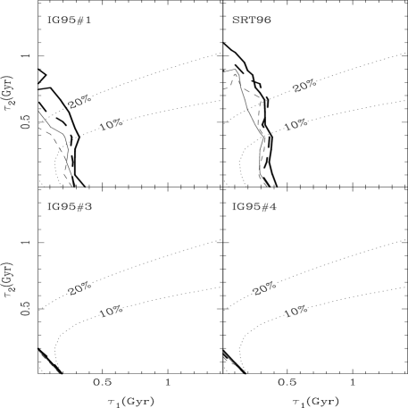
Figure 3: Probability maps at the $90\%$ and $95\%$ (thick) confidence levels in the ($\tau_{1}$,$\tau_{2}$) parameter space for the $C_{\rm eff}=10$,$z_{F}=5$ (solid) and $C_{\rm eff}=10$, $z_{F}=2$ (dashed) models. The dotted lines give the fraction of stars younger than 10 Gyr. The panels show the analysis for all the fields listed in table 1. The analysis is performed with the sample comprising subsolar metallicities.

4 Comparing model and data

We compare the samples discussed above with our model prediction by performing a Kolmogorov-Smirnov (KS) test. The computational method is rather intensive. Furthermore, there is a degeneracy between infall timescale and star formation efficiency so that the width of the metallicity distribution depends on the ratio of these two parameters (see e.g. Lynden-Bell 1975). We can break this degeneracy by using the independent evidence of the age distribution in the Galactic bulge, specifically the low fraction of young and intermediate-age stars inferred from deep colour-magnitude diagrams (Feltzing & Gilmore 2000; Kuijken & Rich 2002; van Loon et al. 2003). We can thus assume a fixed (and high) value of $C_{\rm eff}$, leaving the infall timescale as a free parameter. Hence, we decided to fix the star formation efficiency ($C_{\rm eff}$) and formation epoch ($z_{F}$) for three models, namely ($C_{\rm eff}=10$,$z_{F}=5$), ($C_{\rm eff}=5$,$z_{F}=5$), and ($C_{\rm eff}=10$,$z_{F}=2$). The remaining three parameters are explored over a wide range: $0.01<\tau_{1,2}/{\rm Gyr}<1.5$; $0.0<B_{\rm out}<0.8.$. Models with $C_{\rm eff}=10$; $\tau_{1}=\tau_{2}=0.5$ Gyr form 50% of the stars in $\sim 0.75$ Gyr, compared to a longer duration of $\sim 1.9$ Gyr when the efficiency is lowered to $C_{\rm eff}=1$.

We computed a grid of $16\times 16\times 16$ star formation histories and compared the simulated metallicity histograms with the data described above. The calibration of stars with inferred supersolar iron abundances is rather complicated and implies large uncertainties. Hence, two subsamples of the data were used for each field: one in which all observed stars were included and a second set in which only stars with subsolar iron abundances were included in the histograms. We obtained a final 3D array with each element representing the KS probabilities for a given choice of parameters $(\tau_{1},\tau_{2},B_{\rm out})$. Table 2 gives the 90% confidence levels for these parameters, using only stars with subsolar iron abundances. The results obtained in a comparison with the full sample is shown in table 3. A KS test is an optimal statistic to be used with unbinned data. However, given that different statistical tests are sensitive to different properties of the distribution, we also performed a $\chi^{2}$ test on binned samples. This test is rather dependent on binning. However, the number of stars in each sample is large enough (table 1) to make the comparison worthwhile. We computed the $\chi^{2}$ by taking 10 bins in the range $-3<[$Fe/H$]<+1$ in the metallicity distributions of both the observed data and the models. The parameters we obtained using a $\chi^{2}$ test were very similar to those shown in tables 2 and 3 and always within the 95% confidence levels. Hence, we consider the best fit parameters obtained to be rather insensitive to the statistical estimator used.

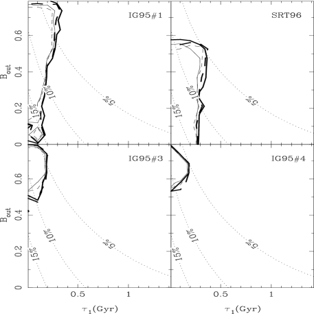
Figure 4: Probability maps at the $90\%$ and $95\%$ confidence levels in the ($\tau_{1}$,$B_{\rm out}$) parameter space. The same notation as in Figure 3 is used.

Figures 3,4, and 5 give probability maps of the KS test at the 90% (thin) and 95% (thick) confidence levels. Two models are given: $C_{\rm eff}=10$, $z_{F}=5$ (solid) and $C_{\rm eff}=10$, $z_{F}=2$ (dashed). Each figure shows a 2D projection of the three dimensional volume spanned by ($\tau_{1}$,$\tau_{2}$,$B_{\rm out}$). Figure 3 shows that the model is incompatible with infall timescales longer than $\sim 1$ Gyr. Given the high star formation efficiencies used in the model, this translates into a very short duration of the star formation stage. The results are rather insensitive to the formation epoch chosen. Tables 2 and 3 show that the best fit parameters are roughly the same for $z_{F}=5$ or $z_{F}=2$ as long as the same star formation efficiency is chosen. This reflects that fact that the stellar metallicity distribution is mostly sensitive to the duration of star formation and does not depend much on absolute ages. A lower star formation efficiency results in longer infall timescales, as seen in the tables. These timescales are still shorter than 1 Gyr at the 90% confidence level for the more reliable subsolar metallicities, except for field SRT96.

The available colour-magnitude diagrams for lines-of-sight in the bulge ranging from projected distances from the Galactic Center of $\sim 100$ pc to many kpc, imply that the vast bulk of the bulge stars are old, with ages greater than $\sim 10$ Gyr (Ortolani et al. 1995; Feltzing & Gilmore 2000; Kuijken & Rich 2002; van Loon et al. 2003). We incorporate these results into the comparison between models and data in terms of a simple fraction of stars predicted to be younger than 10 Gyr, shown as dotted lines in the figures. These mass fractions are computed for a model with $C_{\rm eff}=10$; $z_{F}=2$ and, where applicable, the other parameters are fixed to $B_{\rm out}=0$ (figure 3); $\tau_{2}=0.5$ Gyr (figure 4) or $\tau_{1}=0.5$ Gyr (figure 5). These parameters were chosen to represent a conservative scenario in the estimates of young stellar mass fractions. Hence, the figures show that the assumption of a stellar mass fraction no greater than 20% in stars younger than 10 Gyr imposes a further constraint on the infall timescales, so that $\tau_{2}\lower 2.15277pt\hbox{$\;\buildrel>\over{\sim}\;$}0.5$ Gyr would be ruled out. The estimates for the infall timescales shown in the tables do not take this constraint into account. However, it is worth pointing this out as an additional factor favouring very short infall timescales.

Table 2: Best fit parameters ([Fe/H]$<0$; 90% confidence levels)

FIELD	Model	$\tau_{1}$/Gyr	$\tau_{2}$/Gyr	$B_{\rm out}$
IG95/#1	C10z5	$<0.19$	$<0.51$	$0.48^{+0.24}_{-0.34}$
	C5z5	$<0.40$	$<0.79$	$0.43^{+0.29}_{-0.21}$
	C10z2	$<0.17$	$<0.47$	$0.48^{+0.23}_{-0.33}$
SRT96	C10z5	$<0.26$	$<0.75$	$0.11^{+0.39}_{-0.11}$
	C5z5	$<0.79$	$<1.03$	$0.05^{+0.45}_{-0.05}$
	C10z2	$<0.25$	$<0.74$	$0.32^{+0.17}_{-0.32}$
IG95/#3	C10z5	$<0.09$	$<0.10$	$0.69^{+0.04}_{-0.17}$
	C5z5	$<0.15$	$<0.18$	$0.64^{+0.10}_{-0.10}$
	C10z2	$<0.10$	$<0.10$	$0.69^{+0.04}_{-0.18}$
IG95/#4	C10z5	$<0.10$	$<0.10$	$0.69^{+0.04}_{-0.15}$
	C5z5	$<0.10$	$<0.10$	$0.69^{+0.04}_{-0.15}$
	C10z2	$<0.09$	$<0.08$	$0.69^{+0.03}_{-0.15}$
Z03	C10z5	$<0.16$	$<0.33$	$0.16^{+0.21}_{-0.16}$
	C5z5	$<0.24$	$<0.51$	$0.05^{+0.35}_{-0.05}$
	C10z2	$<0.17$	$<0.37$	$0.05^{+0.41}_{-0.05}$

5 Discussion

5.1 The formation history of the bulge

Figure 6 explores the effect of varying the parameters used in this paper, on the stellar metallicity distribution. In all panels, the dashed line gives the distribution of IG95 field #1. The solid lines are model predictions. The top, left panel gives the best fit from our model to the data, corresponding to $\tau_{1}=\tau_{2}=0.05$ Gyr; $B_{\rm out}=0.5$; $C_{\rm eff}=10$ (for a fixed $z_{F}=5$). The remaining three panels show the predicted histograms when varying any of the parameters explored in this paper, keeping all other parameters fixed to the best fit values. We also show – as a comparison – the histogram of the Z03 field. In the bottom, right panel, the fraction of gas and metals ejected in outflows is changed to $B_{\rm out}=0$ (keeping all other parameters unchanged). The resulting histogram corresponds – to first order – to an offset towards higher metallicities, since more gas is allowed to be locked into subsequent generations of stars. The shape of the histogram will also be slightly modified since a low value for the outflow fraction allows a longer duration of star formation. On the other hand, changing the stellar yields would mimic a change in $B_{\rm out}$, so that given the uncertainties in the Fe yields from simulations of supernova explosions (Woosley & Weaver 1995; Thielemann et al. 1996; Iwamoto et al. 1999) we can conclude that the absolute determination of $B_{\rm out}$ may still carry an important systematic offset. The bottom, left panel of figure 6 shows the effect of a lower star formation efficiency. The histogram does not change much – to be expected given the very short infall timescale considered – although the lower $C_{\rm eff}$ tends to give lower metallicities. We will show below that these models can also be discriminated if [Mg/Fe] abundance ratios are used in the analysis.

The shape of the metallicity distribution is strongly affected by a change in the infall timescale (cf. the infall solution to the local disk ‘G-dwarf problem’, Tinsley 1975). Instead of varying $\tau_{1}$ and $\tau_{2}$ separately, we show on the top, right panel the effect of extending the total infall timescale $\tau_{f}=\tau_{1}+\tau_{2}$ to 1 Gyr. A more extended infall results in a higher fraction of stars with higher [Fe/H], thereby sharpening the metallicity distribution. The prominent tail of the histogram observed at low metallicities shows that long infall timescales are not allowed by the observations. Quantitatively, figure 6 shows that star formation timescales longer than 1 Gyr are unlikely. Notice that field Z03 features a narrower distribution of metallicities, thereby favouring longer infall timescales. However, as shown in table 2 the analysis of the (more reliable) sample comprising stars with subsolar metallicities still discard infall timescales $\tau_{f}\lower 2.15277pt\hbox{$\;\buildrel>\over{\sim}\;$}1$ Gyr for field Z03 at the 90% confidence level. It is also worth remembering that these theoretical distributions assume a very high star formation efficiency – as expected from the lack of young stars in the Galactic bulge. A lower value of $C_{\rm eff}$ will imply a wider distribution of metallicities as $\tau_{f}$ is increased. It is only the case of a very high $C_{\rm eff}$ along with the assumption of instantaneous mixing that gives narrow distributions when extended infall is assumed.

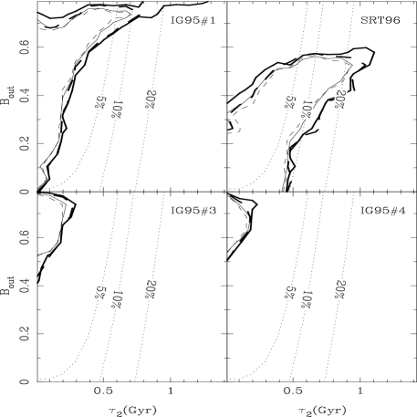
Figure 5: Probability maps at the $90\%$ and $95\%$ confidence levels in the ($\tau_{2}$,$B_{\rm out}$) parameter space. The same notation as in Figure 3 is used.

Table 3: Best fit parameters (All [Fe/H]; 90% confidence levels)

FIELD	Model	$\tau_{1}$/Gyr	$\tau_{2}$/Gyr	$B_{\rm out}$
IG95/#1	C10z5	$<0.18$	$<0.28$	$0.43^{+0.10}_{-0.13}$
	C5z5	$<0.31$	$<0.44$	$0.43^{+0.11}_{-0.11}$
	C10z2	$<0.17$	$<0.27$	$0.43^{+0.09}_{-0.15}$
SRT96	C10z5	$<0.35$	$<0.45$	$0.11^{+0.10}_{-0.11}$
	C5z5	$<1.14$	$<0.74$	$0.11^{+0.12}_{-0.11}$
	C10z2	$<0.28$	$<0.46$	$0.11^{+0.08}_{-0.11}$
IG95/#3	C10z5	$<0.09$	$<0.10$	$0.64^{+0.04}_{-0.11}$
	C5z5	$<0.13$	$<0.18$	$0.64^{+0.05}_{-0.10}$
	C10z2	$<0.09$	$<0.10$	$0.64^{+0.04}_{-0.11}$
IG95/#4	C10z5	$<0.09$	$<0.09$	$0.59^{+0.03}_{-0.12}$
	C5z5	$<0.10$	$<0.13$	$0.59^{+0.04}_{-0.12}$
	C10z2	$<0.09$	$<0.09$	$0.59^{+0.03}_{-0.14}$
Z03	C10z5	$<0.36$	$<0.66$	$0.59^{+0.05}_{-0.10}$
	C5z5	$<1.15$	$<1.02$	$0.59^{+0.05}_{-0.12}$
	C10z2	$<0.36$	$<0.61$	$0.53^{+0.05}_{-0.05}$

Given that the infall timescales predicted by the models are rather short, we decided to explore the validity of this result by performing the same test on a model which adopts the instantaneous recycling approximation (IRA; Tinsley 1980). In the IRA, the stellar lifetimes are assumed to be either zero or infinity, depending on whether the stellar mass is above or below some mass threshold, respectively. In that case, only stars with masses above the threshold will contribute to the enrichment of the subsequent stellar generations. Furthermore, in this approximation we assumed type Ia supernovae do not contribute to the chemical enrichment. Figure 7 shows the result. The probability maps of our full model are shown in the top panels, when comparing stars with subsolar metallicities (right), or the full sample (left) of field IG95/#1. The bottom panels show the result in the IRA. The infall timescales obtained are similar, with $\tau_{1}$ or $\tau_{2}\lower 2.15277pt\hbox{$\;\buildrel>\over{\sim}\;$}0.5$ Gyr ruled out at more than the 90 % confidence level. Hence, the main conclusion of this paper – namely that star formation timescales $\lower 2.15277pt\hbox{$\;\buildrel>\over{\sim}\;$}1$ Gyr are ruled out by the distribution of the metallicities of K giant bulge stars – is a rather robust statement which does not depend critically on the details of the adopted stellar lifetimes.

Figure 6: A comparison of the effect of varying the parameters explored in this paper. The dashed line in all panels give the metallicity distribution of the sample in Ibata & Gilmore field IG95#1. The solid lines are the model predictions. The top-left panel corresponds to $\tau_{1}=\tau_{2}=0.05$ Gyr; $B_{\rm out}=0.5$; $C_{\rm eff}=10$; $z_{F}=5$, which gives a good fit to the observed data (KS test probability $94\%$). The remaining three panels show the predicted histograms when changing one of the parameters to the value shown keeping the other parameters fixed. In the top=right panel, $\tau_{f}$ represents the overall infall timescale $\tau_{1}+\tau_{2}$. Notice infall timescales of $1$ Gyr are readily ruled out because of the narrow metallicity distributions which are generated. The thin line in all four panels give the metallicity distribution of field Z03, which is narrower than IG95#1 thereby allowing for a slightly longer infall timescale.

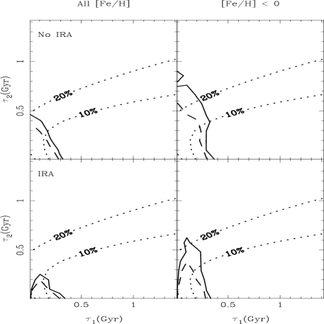
Figure 7: The instantaneous recycling approximation (IRA) assumes stars have either zero or infinite lifetimes depending on whether their masses are larger or smaller than some characteristic mass scale. The bottom panels show the probability maps when comparing the observed metallicity distributions with a model which imposes IRA. We have also set to zero the contribution from type Ia SNe. The top panels show the results from the full model presented in this paper. The figure also shows the difference when including stars with supersolar metallicity to the analysis (left). The solid (dashed) contours represent the 90 (95) % confidence level.

5.2 Linear vs Non-linear Schmidt laws

One could expect that the short timescales obtained in the model presented here could vary significantly when changing the dependence between gas density and star formation. We have used throughout this paper a Schmidt law with an exponent of $1.5$ (equation 2). Figure 8 shows the predicted metallicity distribution when the exponent is changed first to a linear, and secondly to a quadratic, Schmidt law. The difference between the predictions of our fiducial $n=1.5$ model and those with $n=2$ is not large. However, a linear law ($n=1$) gives a significantly sharper histogram, to be expected since a linear law extends the period of star formation for the same amount of gas and star-formation efficiency. Longer star formation timescales (for fixed infall timescales) generate more stars with higher metallicity, thereby making the histogram narrower – much in the same way as more extended infall for a fixed star formation timescale. Therefore, our conclusion regarding the need for short star formation timescales is independent of the exponent used in the Schmidt law. Furthermore, a linear dependence would require even shorter infall timescales !

5.3 Bulge Spectrophotometry

We can use the star formation history that gives the best fit to the observed histograms and convolve it with simple stellar populations over the range of ages and metallicities predicted by the model. We used the latest version of the population synthesis models of Bruzual & Charlot (1993; priv. comm.) in order to generate an integrated spectral energy distribution (sed) as shown in figure 9, which corresponds to $\tau_{1}=\tau_{2}=0.2$ Gyr; $B_{\rm out}=0.5$. The sed has been normalized to the flux in the $B$-band. The resulting sed gives colours $U-V=1.13$; $V-K=2.86$. For comparison purposes we have considered another model with a longer infall timescale ($\tau_{1}=1$ Gyr; dashed line). The colours of this model — $U-V=1.34$; $V-K=2.99$ — are redder because of the higher metallicities caused by longer infall timescales. The dots with error bars are the average and standard deviation of the $U-B$ and $B-V$ colours from the sample of 257 bulges from Sbc spirals of Gadotti & dos Anjos (2001). Our predicted $B-V=0.4$ colour is compatible with the average and standard deviation of the observed colour $B-V=0.64\pm 0.20$ (using a subsample of bulges with negative colour gradients). However, our predicition for $U-B=0.6$ is significantly bluer than the observed $U-B=0.19\pm 0.20$. This may be due to uncertainties in either the chemical enrichment model or the population synthesis models considered. Figures 4 and 5 show that the value of $B_{\rm out}$ is rather uncertain and this has a strong effect in the final colours. Furthermore, the discrepancy towards bluer observed colours may be caused by a systematic disk contamination in the observations. Even though less than 5% of the $257$ bulges observed by Gadotti & dos Anjos (2001) have colours $U-B<0.5$, a comparison with the colours of early-type galaxies $U-B\sim 0.6-0.7$ (e.g. González 1993) shows that our model predictions are compatible with the photometry of spheroids.

Figure 9 illustrates the challenging task of estimating infall timescales from $UBV$ broadband photometry alone. Only the spectral window around $2000$Å  could be useful in order to rule out formation timescales longer than $1$ Gyr. In that spectral region, the differences can be as large as $1$ magnitude although the analysis would be hindered by the many uncertainties behind the model of star formation and chemical enrichment as well as by the uncertainties in the model predictions from population synthesis models. The direct comparison of stellar metallicites is thereby a much more powerful technique to infer the star formation history of a bulge, stellar cluster, or galaxy.

Figure 8: Metallicity distribution predicted for three different exponents of the Schmidt law relating the star formation rate with the gas density. The model corresponds to $\tau_{1}=\tau_{2}=0.1$ Gyr; $B_{\rm out}=0.5$; $C_{\rm eff}=10$. Notice that a linear law gives a much sharper histogram since star formation takes longer for the same amount of gas, compared to a non-linear law with $n>1$.

5.4 Simple Model and the duration of star formation

The broad tail of the metallicity distribution at low values of [Fe/H] could imply that the Galactic bulge can be reasonably fit by the so-called Simple Model (e.g. Pagel 1997), which assumes a closed box system and the instantaneous recycling approximation. The beauty of the model lies in the ability to generate a metallicity distribution which is completely independent of the star formation history. The histogram is thereby degenerate with respect to the duration of the star formation process. It only depends on the total stellar yield $y$ as a scale factor in the following way:

$$\frac{dM_{\star}}{d\log Z}\propto(Z/y)\exp(-Z/y),$$ (15)

where $Z$ is the total metallicity and $M_{\star}$ is the stellar mass content. This distribution has a rather broad range of low-metallicity stars, which has been the reason why a Simple Model was discarded to explain the formation of the local Galactic disk as it generated too many G-dwarf stars at low metallicities (e.g. Tinsley 1980). However, the bulge distributions shown in figure 2 are broader and so, more compatible with this model.

We compared the best fits of a Simple Model with those from our infall model in figure 10. We plot the Kolmogorov-Smirnov probability when comparing fields IG95#1 (top) and SRT96 (bottom) with our model for a fixed formation redshift: $z_{F}=5$, $\tau_{1}=0.1$ Gyr. The outflow parameter was chosen to maximise the probability for each field. We take $B_{\rm out}=0.5$ for IG95#1 and $B_{\rm out}=0$ for SRT96. Three different star formation efficiencies are considered, namely $C_{\rm eff}=\{5,10,20\}$. The KS probability is shown as a function of $\tau_{2}$ (left) or $\Delta t_{\rm SF}$ (right), where the latter is defined as the time lapse during which 75% of the total stellar mass content in the bulge is generated. Only sub-solar metallicities are considered in the test. The horizontal line gives the highest probability for a Simple Model, varying the yield ($y$) in order to maximize the probability. Hence, one can see that our models give better fits than a Simple Model, so that a detailed analysis of the metallicity distribution in the bulge can be used to set limits on the duration of star formation. All models shown in the figure give star formation timescales shorter than $\sim 1.5$ Gyr. Furthermore, the [Mg/Fe] enhancement observed in bulge stars (Rich & McWilliam 2000) speaks in favour of models with a high $C_{\rm eff}$ so that star formation timescales $\Delta t_{\rm SF}\lower 2.15277pt\hbox{$\;\buildrel<\over{\sim}\;$}0.5$ Gyr are expected.

Figure 9: Spectral energy distribution (sed) obtained by convolving the star formation history for the best fit to Ibata & Gilmore field IG95#1 with the stellar population synthesis models of Bruzual & Charlot (in preparation). The model corresponds to $\tau_{1}=\tau_{2}=0.05$ Gyr; $B_{\rm out}=0.5$. The vertical lines give the central positions of the $U$, $B$, and $V$ passbands. A second sed with a longer timescale ($\tau_{1}=1$ Gyr) is also shown (dashed line). The larger population of stars with a higher metallicity in the $\tau_{1}=1$ Gyr model is responsible for the redder colours. The dots correspond to the average and standard deviation of the Sbc bulge sample of Gadotti & dos Anjos (2001). A comparison of the solid and dashed lines shows that it is very difficult to determine SFH parameters from integrated spectroscopy alone. The distribution of stellar metallicities (as presented in this paper) is a much more sensitive discriminator.

6 Conclusions

We have explored a simple model describing the formation and evolution of the stellar populations of the Galactic bulge using a set of a few parameters. A comparison of the model predictions with the observed [Fe/H] distribution of K giants in various fields towards the bulge requires relatively short infall timescales ($\lower 2.15277pt\hbox{$\;\buildrel<\over{\sim}\;$}0.5$ Gyr) regardless of the field considered (Figure 3). Our model compares the resulting star formation history and subsequent enrichment with the distribution of stellar metallicities. Within the model assumptions and other uncertainties, one can relate the infall timescales with the duration of star formation. Hence, formation timescales longer than $\lower 2.15277pt\hbox{$\;\buildrel>\over{\sim}\;$}1$ Gyr are ruled out at more than the 90 % confidence level regardless of the field, statistical test, or on whether stars with supersolar metallicities are excluded from the analysis (Figure 7).

Figure 10: Comparison of the Kolmogorov-Smirnov probability as a function of $\tau_{2}$ (left) or $\Delta t_{\rm SF}$ (right). The latter gives the time for the bulge to generate 75% of the total stellar mass content. Fields IG95#1 (top) and SRT96 (bottom) are tested with a fixed value of $B_{\rm out}=0.5$ (IG95#1) and $B_{\rm out}=0$ (SRT96) and $\tau_{1}=0.1$ Gyr, $z_{F}=5$ for both fields. Three star formation efficiencies are chosen, namely $C_{\rm eff}=5$ (dashed), $10$ (dotted), and $20$ (solid). The horizontal line gives the best fit for a Simple Model.

Outflows during the formation of the bulge can also be estimated, although this result is very strongly dependent on the (uncertain) absolute stellar yields of Fe from type II supernovae and requires a precise calibration of the absolute metallicities of the observed stars, including the effect of non-solar abundance ratios. Taking the derived distributions as face value, even if we decided to track the total metallicity, $Z$, instead of the Fe content, the uncertainties in the stellar yields from intermediate mass stars are still large enough so that the model estimates of the fraction of gas and metals ejected in outflows are more qualitative than quantitative. Nevertheless, we find outflows may be very significant in most of the fields studied. Baade’s window (SRT96) is the field in which high outflow fractions are ruled out. On the other hand, the fields from IG95 favour a large amount of gas ejected in outflows. In these fields, $B_{\rm out}\sim 0.5-0.7$ give the best fit, and $B_{\rm out}=0$ seems to be a very unlikely scenario even if the real stellar yields or the IMF are far from those adopted in this paper. This difference in outflow fraction is in the sense expected if outflow is inhibited in the deepest part of the potential well. Large outflow fractions are expected and predicted in some models that include estimates of the dynamical effects of feedback from stars (e.g. Arimoto & Yoshii 1987). It is worth noticing that these values of $B_{\rm out}$ imply a very significant amount of metals contributing to the enrichment of the IGM (Renzini 1997), provided the gas escapes the overall Galaxy, rather than for example enriching the disk.

The short timescales predicted by the analysis of the metallicity distribution of bulge stars has a direct consequence on abundance ratios such as [Mg/Fe]. This ratio is a reasonably robust indicator of the duration of star formation. Solar values are achieved when extended star formation takes place, so that the debris from SNeIa can be incorporated into subsequent generations of stars. On the other hand, short-lived bursts such as the one we predict in this paper, translates into enhanced [Mg/Fe] in most bulge stars. Figure 11 shows this point. Analogously to figure 6, we give the model prediction for various choices of the parameters including the set that gives the best fit. In this case the histogram of [Mg/Fe] is shown. In most cases, the distribution is very similar, peaked at [Mg/Fe]$\sim+0.25$ with an extended tail which dies off at solar abundance ratios. Only the model with low star formation efficiency (bottom left) gives a significantly different histogram. A low $C_{\rm eff}$ implies a more extended period of star formation, generating a broader histogram as more stars become polluted by SNeIa ejecta. The abundance ratios observed by Rich & McWilliam (2000) on a sample of bulge giants using Keck/HIRES rule out models with low star formation efficiencies.

The main outcome of this paper is that infall timescales $\tau\lower 2.15277pt\hbox{$\;\buildrel>\over{\sim}\;$}1$ Gyr are ruled out by the observed metallicity distribution of the Galactic bulge. Short star formation times are also to be expected given the observed broad distribution of the metallicities of bulge K giants. The preferred value stays around infall timescales $\tau_{f}\sim 0.1-0.2$ Gyr, which would correspond to star formation timescales $\tau_{\rm SF}\lower 2.15277pt\hbox{$\;\buildrel<\over{\sim}\;$}1$ Gyr. However, the differences between the iron-abundance distributions from the different fields explored in this paper illustrate the need for a uniform large-scale (IR) spectroscopic survey, with radial velocity AND STAR COUNTS used as an aid to the statistical separation of bulge and foreground disk AND STELLAR HALO.

Figure 11: Distribution of [Mg/Fe] abundances predicted by the models shown in figure 6. The histogram corresponding to the best fit is shown in the top-left panel as well as in the three remaining panels as a dashed line. Notice that a low star formation efficiency – which generates a similar [Fe/H] as the best fit as seen in figure 6 – generates a very wide [Mg/Fe] distribution.

A robust calibration of metallicities – which should account for variations in the [$\alpha$/Fe] abundance ratios – is crucial in the quantification of the amount of gas ejected in outflows during the formation of the bulge. Furthermore, an accurate distribution of abundance ratios such as [Mg/Fe] (figure 11) would pose strong constraints on the duration of the star formation burst which gave way to the Galactic bulge.

Our technique is quite robust and complementary to a comparison of the stellar colour-magnitude diagrams of old populations. The latter can only constrain the star formation timescale to a few Gyr due to the crowding of the isochrones at old ages. The model presented here sets strong constraints for bulge formation in semi-analytical models, the latest of which predict formation timescales for bulges significantly longer than these timescales (Abadi et al. 2002). Furthermore, secular evolution models predict formation times which extend over many dynamical timescales. Hence, formation scenarios over times $\sim 0.1-0.2$ Gyr, as presented here, would be in conflict with bulge formation from bar instabilities. Our results for the buildup of the Galactic bulge favour formation scenarios in which a strong starburst quickly converts all gas available into stars in a few dynamical timescales (Elmegreen 1999).

References

- (1) Abadi, M. G., Navarro, J. F., Steinmetz, M. & Eke, V. R., 2002, astro-ph/0212282
- (2) Arimoto, N. & Yoshii, Y., 1987, A&A, 173, 23
- (3) Bruzual, A. G. & Charlot, S., 1993, ApJ, 405, 538
- (4) Ellis, R. S., Abraham, R. G. & Dickinson, M., 2001, ApJ, 551, 111
- (5) Elmegreen, B. G., 1999, ApJ, 517, 103
- (6) Faber, S. M., Friel, E. D., Burstein, D. & Gaskell, C. M., 1985, ApJS, 57, 711
- (7) Feltzing, S. & Gilmore, G., 2000, A&A, 355, 945; erratum 2001, A&A, 369, 510
- (8) Ferreras, I. & Silk, J., 2000a, ApJ, 532, 193
- (9) Ferreras, I. & Silk, J., 2000b, MNRAS, 316, 786
- (10) Ferreras, I. & Silk, J., 2001, ApJ, 557, 165
- (11) Fukugita, M., Hogan, C. & Peebles, P. J., 1998, ApJ, 503, 518
- (12) Gadotti, D. A. & dos Anjos, S., 2001, AJ, 122, 1298
- (13) González, J. J., 1993, Ph.D. thesis, UC Santa Cruz
- (14) Greggio, L. & Renzini, A., 1983, A&A, 118, 217
- (15) Hartwick, F. D. A., 1976, ApJ, 209, 418
- (16) Ibata, R. A. & Gilmore, G. F., 1995a, MNRAS, 275, 591 (IG95)
- (17) Ibata, R. A. & Gilmore, G. F., 1995b, MNRAS, 275, 605
- (18) Iben, I. & Tutukov, A., 1984, ApJS, 54, 335
- (19) Iwamoto, K., Brachwitz, F., Nomoto, K., Kishimoto, N., Umeda, H., Hix, W. R., Thielemann, F.-K., 1999, ApJS, 125, 439
- (20) Kuijken, K., & Rich, R. M., 2002, AJ, 124, 2054
- (21) Kauffmann, G., 1996, MNRAS, 281, 487
- (22) Kennicutt, R. C., 1998, ApJ, 498, 541
- (23) Larson, R. B., 1974, MNRAS, 169, 229
- (24) Lynden-Bell, D., 1975, Vistas in Astronomy 19, 299
- (25) McNamara, D. H., Madsen, J. B., Barnes, J. & Ericksen, B. F., 2000, PASP, 112, 202
- (26) McWilliam, A. & Rich, R.M. 1994, ApJS, 91, 749
- (27) Maraston, C., et al. 2003, A&A in press (astro-ph/0209220)
- (28) Matteucci, F. & Greggio, L., 1986, A&A, 154, 279
- (29) Matteucci, F. & Recchi, S., 2001, ApJ, 558, 351
- (30) Matteucci, F., Romano, D. & Molaro, P., 1999, A&A, 341, 458
- (31) Mollá, M., Ferrini, F. & Gozzi, G., 2000, MNRAS, 316, 345
- (32) Mould, J. R., 1984, PASP, 96, 773
- (33) Nomoto, K., Iwamoto, K. & Kishimoto, N., 1997, Science, 276, 1378
- (34) Norman, C. A., Sellwood, J. A. & Hasan, H., 1996, ApJ, 462, 114
- (35) Ortolani, S., Renzini, A., Gilmozzi, R., Marconi, G., Barbuy, B., Bica, E. & Rich, R. M., 1995, Nature, 377, 701
- (36) Pagel, B. E. J. “Nucleosynthesis and chemical evolution of galaxies”, 1997, Cambridge, p. 218
- (37) Peletier, R. F., Balcells, M., Davies, R. L., Andredakis, Y., Vazdekis, A., Burkert, A. & Prada, F., 1999, MNRAS, 310, 703
- (38) Proctor, R. N., Sansom, A. E. & Reid, I. N., 2000, MNRAS, 311, 37
- (39) Raha, N., Sellwood, J. A., James, R. A. & Kahn, F. D., 1991, Nature, 352, 411
- (40) Renzini, A. 1997, ApJ, 488, 35
- (41) Rich, R. M., 1990, ApJ, 362, 604
- (42) Rich, R. M. & McWilliam, A., 2000, Proc. SPIE, 4005, 150
- (43) Sadler, E. M., Rich, R. M. & Terndrup, D. M., 1996, AJ, 112, 171 (SRT96)
- (44) Salaris, M., Chieffi, A. & Straniero, O., 1993, ApJ, 414, 580
- (45) Salpeter, E. E. 1955, ApJ, 121, 161
- (46) Scalo, J. M. 1986, Fund.Cosm.Phys. 11, 1
- (47) Schaller, G., Schaerer, D., Maeder, A. & Meynet, G. 1992, A&AS, 96, 269
- (48) Schmidt, M. 1959, ApJ 129, 243
- (49) Shapiro, S. L. & Teukolsky, S. A. 1983, Black Holes, White Dwarfs and Neutron Stars, New York, Wiley-Interscience
- (50) Thielemann, K. F., Nomoto, K. & Hashimoto, M. 1996, ApJ, 460, 408
- (51) Tinsley, B. M. 1975, ApJ, 197, 159
- (52) Tinsley, B. M. 1980, Fund.Cosm.Phys., 5, 287
- (53) Tutukov, A. V. & Yungelson, L. R. 1980, in Close binary stars, IAU symp. no. 88, eds. M. J. Plavec, D. M. Popper and R. K. Ulrich, Reidel, Dordrecht, p.15
- (54) van Loon, J. Th., et al. 2003, MNRAS, 338, 857
- (55) Woosley, S. & Weaver, T. 1995, ApJS, 101, 181
- (56) Zoccali, M., et al., 2003, A&A, 399, 931