Do We Live in a Vanilla Universe?
Theoretical Perspectives on WMAP

Abstract

I discuss the theoretical implications of the WMAP results, stressing WMAP’s detection of a correlation between the E-mode polarization and temperature anisotropies, which provides strong support for the overall inflationary paradigm. I point out that almost all inflationary models have a “vanilla limit,” where their parameters cannot be distinguished from a genuinely de Sitter inflationary phase. Because its findings are consistent with vanilla inflation, WMAP cannot exclude entire classes of inflationary models. Finally, I summarize hints in the current dataset that the CMB contains relics of new physics, and the possibility that we can use observational data to reconstruct the inflaton potential.

1 Introduction

On February 12, 2003, the Wilkinson Microwave Anisotropy Probe [WMAP] reported results based on its first year of observations (e.g. Bennett:2003bz ; Spergel:2003cb ; Hinshaw:2003ex ; Peiris:2003ff ; Kogut:2003et ), and cosmology took a giant step towards its long promised “golden age.” Ref. Spergel:2003cb lists the values of 22 cosmological parameters determined using the WMAP data and other recent observational information. Many of these values are quoted with several significant figures, whereas a decade ago they were either completely undetermined or had massive uncertainties.

For the theoretical cosmologist, the WMAP results are more tantalizing than revolutionary. On the one hand, WMAP confirms that there is a significant contribution from dark energy in the present epoch, puts tight constraints on the parameter space open to inflation, and provides strong support to the overall inflationary paradigm. However, this does not surprise most theoreticians, and nothing in the current WMAP dataset puts genuinely nontrivial constraints on the physics of inflation and the very early universe.

To explain further, consider vanilla inflation – an almost exactly de Sitter inflationary epoch which lasts long enough to deliver a primordial universe – whose measurable parameters all have their “default values”. After vanilla inflation, scalar perturbations are Gaussian and scale-free, and there is no discernible contribution from tensor modes or curvature in the present epoch. Consequently, all parameters which constrain the primordial universe would be measured as upper bounds, rather than definite values.

Almost all inflationary models have parameters which can be tuned to provide a vanilla limit. In some cases these tunings may appear so unnatural, and one may want to exclude the model on aesthetic grounds. For instance, the perturbation spectrum associated with a $\phi^{n}$ potential becomes more strongly scale dependent as $n$ increases, and one may argue that $n$ should be an even, positive number. The vanilla limit of this model is $n\rightarrow 0$, so if $n\geq 2$ is experimentally excluded, the model becomes less attractive. However, this prejudice is far less compelling than the observation of an unambiguously blue spectrum (one with more power on short scales than on long scales): in this case all positive values of $n$ are excluded. The one type of inflation which is hard to tune is de Sitter inflation, where the inflaton is trapped in a local minimum of the potential and does not evolve at all. However, in this case the spectrum is precisely scale invariant, which is the vanilla result.

Vanilla inflation has an ambiguous position in theoretical cosmology. It has the most “natural” set of parameter values but offers the smallest leverage for discriminating between different realisations of inflation, and thus the least insight into the early universe. Consequently, theoreticians tend to seize on any hints that the inflationary epoch contains non-vanilla flavorings, since these significantly constrain the inflationary parameter space and, in extreme cases, challenge the overall paradigm. The first year WMAP dataset has two tantalizing features: the apparent lack of power at long wavelengths, and the suggestion that the scalar spectral index itself is a function of the perturbation’s wavelength.

2 The CMB and Inflation

Almost any possible inflationary epoch can be described in terms of a scalar field $\phi$ moving in a potential, $V(\phi)$. From the Einstein field equations and the energy momentum tensor for a minimally coupled scalar field once can deduce

$$H^{2}=\left({\dot{a}\over a}\right)^{2}={8\pi\over 3m_{\rm Pl}^{2}}\left[{1\over 2}\dot{\phi}^{2}+V(\phi)\right],$$ (1)

where $a(t)$ is the spacetime scale factor, and a dot denotes differentiation with respect to time. We are implicitly assuming a spatially flat, homogeneous and isotropic universe where the inflaton field is the only contribution to the energy-momentum tensor. The motion of the field is given by

$$\ddot{\phi}+3H\dot{\phi}+V^{\prime}(\phi)=0,$$ (2)

where the dash notes differentiation with respect to $\phi$.

Guth’s original paper on inflation Guth:1980zm addressed problems associated with the dynamics of the cosmological background. Inflation can be implemented in a multitude of different ways, all of which solve the cosmological problems addressed by Guth. Consequently, inflationary model builders do not focus directly on the expansion history of the universe. In addition to the zero-order dynamics needed to set the stage for a hot big-bang universe, inflation also predicts the first order perturbations about this background solution. These perturbations determine both the clustering properties of galaxies, and the anisotropies in the microwave background.

Inflation produces primordial perturbations by magnifying quantum fluctuations until their wavelength is equal to or larger than the present size of the observable universe. The properties of these fluctuations differ markedly between different inflationary models and specific inflationary scenarios can thus be distinguished from one another and tested via their perturbation spectra. Consequently, putting tight experimental constraints on the perturbation spectrum is of prime importance, since the theoretical cosmologist can use this data to eliminate specific inflationary models. However, almost all inflationary models have a vanilla limit, so as long as vanilla inflation remains consistent with the observational data we cannot exclude entire classes of models.

Given the functional form of the potential and fairly mild assumptions about the dynamics of inflation, we express the perturbation spectra as a function of the potential and its derivatives. A general perturbation to the background $g_{\mu\nu}$ is a symmetric tensor, $h_{\mu\nu}$, where the perturbed spacetime is $g_{\mu\nu}+h_{\mu\nu}$ Mukhanov:1990me . We decompose $h$ into scalar, vector and anti-symmetric tensor components, where the decomposition reflects the transformation properties of the different pieces under (small) transformations. Cosmologically, we need consider only the scalar and tensor modes, as the vector modes decay with time. The scalar modes are associated with a gravitational potential and are the source of density fluctuations in the universe. The tensor modes are effectively gravity waves (and are often referred to as such) and do not contribute to the formation of structure in the universe, but do contribute to the microwave background anisotropies, especially at large angular scales.

The perturbations are described in terms of their power spectra,

$$P_{S}^{1/2}\sim k^{n_{S}-1},\quad P_{T}^{1/2}\sim k^{n_{T}}$$ (3)

where $k$ is the comoving wavenumber of the perturbation. If $n_{S}=1$ or $n_{T}=0$ the amount of power in each mode is independent of $k$ and the resulting spectra are scale invariant. We know that the underlying spectra must be roughly scale invariant, but the question is whether the difference between $n_{S}$ and $n_{T}$ from their “natural” values of 1 and 0 is detectable observationally.

Using the slow roll approximation, we can write $n_{S}$ and $n_{T}$ in terms of derivatives of the potential Lidsey:1995np ,

$$n_{S}=1+2\eta-4\epsilon,\qquad n_{T}=-2\epsilon$$ (4)

where

$$\epsilon=\frac{m_{p}^{2}}{16\pi}\left(\frac{V^{\prime}}{V}\right)^{2}\,,\quad\eta=\frac{m_{p}^{2}}{8\pi}\left[\frac{V^{\prime}}{V}-\frac{1}{2}\left(\frac{V^{\prime}}{V}\right)^{2}\right].$$ (5)

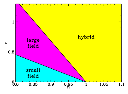
Figure 1: The three classes of single field inflationary models are displayed. The hybrid models have $\eta>\epsilon>0$, and the small field models have $\eta<0$. Vanilla inflation corresponds to $r=0$ and $n=1$, the point at which the three wedges intersect. (Plot from Kinney:1998md .)

Finally, the amplitudes of the two spectra must obey a consistency condition,

$$\frac{P_{T}^{1/2}}{P_{S}^{1/2}}=16\epsilon$$ (6)

where the numerical coefficient is, to some extent, a matter of definition. We can divide inflationary models into three general classes, summarized in Figure 1 Kinney:1998md . In the hybrid case, the $V^{\prime\prime}/V\gg(V^{\prime}/V)^{2}$, and the field is evolving towards a local minimum of the potential. Conversely, if we find $n_{S}<1$ and no detectable tensor contribution, $V^{\prime\prime}<0$ and $V^{\prime}\sim 0$, and we have small field inflation. Finally, if we observe a significant tensor component, we must have $V^{\prime}/V\neq 0$. From the equation of motion for $\phi$, we see that $\dot{\phi}\neq 0$, and the total evolution of $\phi$ during inflation can be substantial – leading to the moniker large field inflation.

While a non-zero scalar spectrum is needed to provide the primordial density fluctuations that seed the formation of structure, a primordial tensor spectrum is optional. We can show that the $P_{T}^{1/2}$ is proproportional to the value of $H$ (and thus the square root of the energy density) during inflation and, unless $H$ is GUT scale or above, the tensor signal will most likely be forever undetectable. Since a detectable tensor signal is produced by a limited range of inflationary models the vanilla prediction is that the CMB contains no detectable contribution from tensors. However, if we do observe a primordial tensor spectrum, then we can immediately deduce the energy scale at which inflation occurred. Moreover, if we can measure both its amplitude and index, we are in the pleasant position of having four observable quantities (the amplitudes and indices of the tensor and scalar spectrum) which are specified in terms of three parameters. This leads to a “consistency condition” which must be satisfied (to first order in slow-roll) by all single field inflationary models.

3 The WMAP Results: Summary

Conceptually, the WMAP mission is very simple: over a period of several years, it makes repeated observations of the microwave sky, and is sensitive to both temperature and polarization. It observes in five frequency bands, since the main foreground contaminants scale differently with frequency from the underlying black body of the CMB.

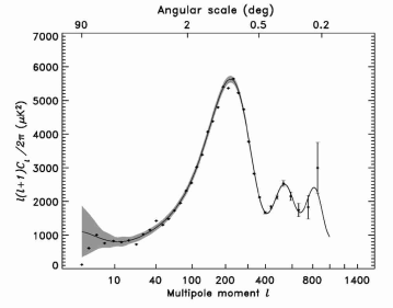
Figure 2: The WMAP power spectrum, where the shaded region represents the expected cosmic variance about the best fit spectrum Hinshaw:2003ex .

Information can be extracted from the maps directly (for instance, the topology of isotemperature contours is a function of the underlying cosmological model Colley:2003sp ), but the maps are frequently distilled into a power spectrum by expanding them in spherical harmonics, and the WMAP power spectrum is shown in Figure 2. Different theoretical models of the early universe predict different scalar and tensor spectra, but the CMB also depends on parameters such as the cosmological constant and the Hubble constant via their influence on the evolution of the perturbations as they propagate in an expanding universe. This is crucial, since it turns the CMB into a tool for estimating a wide range of cosmological parameters which, taken together, put tight constraints on the composition and history of our universe.

Given a set of parameters, the theoretical spectrum is estimated using a tool such as CMBFAST. Armed with high quality CMB data (and data from other sources) one can find the “best fit” model by varying the parameters until the underlying spectrum is matched as accurately as possible. Spergel et al. Spergel:2003cb describes this process. The WMAP team concludes that the age of the universe is $13.7\pm 0.2$Gyr, the total mass-energy of the universe is $\Omega_{tot}=1.02\pm 0.02$ (where a value of unity corresponds to a universe with no spatial curvature), the parameterized Hubble constant $h=0.71^{+0.04}_{-0.03}$, and baryon density (as a fraction of the total energy density) $\Omega_{b}h^{2}=0.0224\pm 0.0009$. Little more than a decade ago, the value of all of these numbers was the subject of significant controversy, and yet here they are all quoted to two or three significant figures.

4 Polarization

Since the first detection of the CMB anisotropies, attention has focussed on the temperature variations. The polarization also varies from point to point, but this anisotropy is intrinsically smaller and more difficult to measure. WMAP is the first full-sky mission to return a non-zero polarization measurement Kogut:2003et .

Figure 3: The cross-correlation between the E-mode polarization and temperature anisotropies in the CMB. The solid line represents the inflationary prediction, while the defect prediction is shown by the dotted line Hinshaw:2003ex .

In a universe where inflation occurs, the primordial perturbations may be correlated on scales far larger than the present size of the observable universe, and were definitely correlated on super-horizon scales when the microwave background photons decoupled from the rest of the universe some 300,000 years after the big bang. While other mechanisms for generating the primordial density perturbations have been explored (particularly “defect models” where objects such as cosmic strings generate perturbations as they move through the universe), these do not produce super-horizon correlations. A frequent critique of inflation is that the overall paradigm makes no generic predictions, and that there is no one property that all inflationary models share. However, a universe with super-horizon perturbations at decoupling has a characteristic correlation between the temperature anisotropies and the E-mode polarization signal. WMAP was observed this correlation, and found that it closely matches the inflationary prediction.

It is worth pausing to reflect what a significant achievement this is: from my perspective the observed correlation between temperature and E-mode polarization is most important single result in the WMAP dataset. Prior to inflation, no-one had predicted super-horizon correlations, so this observation is a stunning verification of one of the key features of inflation. Moreover, if the data had not confirmed the inflationary prediction, almost all models of inflation would have been ruled out in a single stroke. Consequently, this is a key test of the inflationary paradigm. The only downside (and perhaps the reason why more is not being said about it) is that because all inflationary models make this prediction, it only eliminates models such as defect scenarios which have already fallen from favor in the theoretical community. However, I suspect that this observation will be regarded as one of the lasting achievements of WMAP, and that observations of the $\langle TE\rangle$ cross-correlation will be followed carefully as the data improves.

5 Surprises: Non-Vanilla Features in WMAP?

The two obvious peculiarities in the WMAP dataset are that the spectrum has anomalously low power on small scales, and that the fit to the data improves if the scalar index is allowed to be scale-dependent (that is, $n_{s}$ is a function of $k$). Either of these results could provide a dramatic non-vanilla flavor to the early universe. However, in both cases their physical significance is hard to quantify and await both further data and theoretical analysis.

5.1 Low Quadrupole

The low quadrupole is visible in the power spectrum of Figure 2, as the first data points lie well below the best-fit spectrum. Due to cosmic variance, we don’t expect an exact match between theory and experiment at small values of $l$, but the discrepancy is, on the face of it, unexpectedly large.

While it is clear that the observed CMB sky has less power at large wavelengths (low $k$) than that suggested by the “best fit” $\Lambda$CDM model, it is not clear is whether this is something we need to explain, since the result could be produced by cosmic variance alone. Spergel et al. Spergel:2003cb generated multiple realizations of the microwave background with the parameters estimated by WMAP, and found that the probability that the low power at small $l$ is due to cosmic variance is $1.5\times 10^{-3}$. However, other authors (Efstathiou:2003wr , for example) argue that this calculation underestimates cosmic variance, and that the discrepancy is not large enough to be a signal of new physics.

If this result is significant, the possible modifications to the standard paradigm that would suppress power at large scales take a variety of forms. For example, a comparatively conservate approach is provided by Contaldi et al. Contaldi:2003zv , who look at inflationary models which are tuned to suppress $P_{S}$ for values of $k$ which dominate the low $l$ terms in the CMB spectrum. Carefully tuned inflationary models violate the spirit of the inflationary paradigm, but they are less radical departures from the standard cosmology than (for instance) advocating a toroidal universe with a “cell size” that is smaller than the current size of the visible universe deOliveira-Costa:2003pu , or that the universe possesses detectable (and positive) spatial curvature Efstathiou:2003hk , both of which would tend to cut off the power spectrum at long wavelengths.

Simply measuring the microwave sky more accurately will not reduce the cosmic variance. However, it is possible that some of lack of power at low $l$ could be explained by an over-aggressive foreground subtraction, and this is amenable to testing and improvement. Conversely, if the suppression of power at low $l$ is a real effect, evidence for it will appear in other places. For example, Kesden et al. Kesden:2003zm show that the shear produced by gravitational inhomogeneities, which distorts the correlation between temperature and polarization anisotropies, would be measurably different in a universe where the spectrum lacked power at small values of $k$, and this can be tested by future experiments.

5.2 Running Index

The low quadrupole seen by WMAP is suggestive of unsuspected physics that plays a role at large angular scales. However, WMAP also hints that the standard assumption of an underlying spectrum described by a constant index $n_{S}$ may be too simplistic Peiris:2003ff . In this case, the principal evidence is found in CMB data at small angular scales. This is currently dominated by observational uncertainty, rather than cosmic variance. In fact, the first-year WMAP dataset alone does cover a large enough range of $l$-values to provide any evidence for a running ($k$ dependent) $n_{S}$. The evidence for running (between the 1 and 2 $\sigma$ level) appears when the WMAP power spectrum is combined with that derived from galaxy surveys and Lyman-$\alpha$ forest data, both of which provide data on the primordial spectrum at smaller scales than is possible with the CMB alone Peiris:2003ff .

If the running index is confirmed, it will put tight constraints on inflation. The slow roll expansion for the spectral index given by equation (3) can be extended to beyond the leading order result given here, and $dn_{S}/d\ln{k}$ is dependent on the third derivative of the potential. However, having $V^{\prime\prime\prime}(\phi)$ large enough to produce a $dn_{S}/d\ln{k}$ observable by WMAP rules out almost all standard models of inflation. This is not, in itself, a drawback. Moreover, it would comprehensively rule out vanilla inflation, which would be very a welcome development indeed. Moreover, if the potential has a number of “features” then it may not need to be carefully tuned in order to ensure that one of these features is found within the range of $\phi$ covered by the inflaton field as the cosmologically relevant perturbations are generated Adams:2001vc . Indeed, a potential of this sort was considered by the WMAP team, and there is weak support in the WMAP dataset (in combination with other survey information) for this type of feature.

The major caveat about this possible non-vanilla flavoring of the early universe is simply that the data is inconclusive. The result hinges on the merger of several datasets, which increases the complexity of any statistical analysis, and the level of significance is small enough for it to simply be the result of a statistical fluctuation. This uncertainty will soon be resolved – the next year of WMAP data will significantly improve the sensitivity of the measurements of the $C_{l}$ for larger values of $l$, and the SDSS [Sloan Digital Sky Survey] will supplant the galaxy surveys used by the WMAP team in their previous papers.

6 Reconstructing the Potential

One of the principal dreams of the theoretical cosmologist is to reconstruct the underlying physical mechanism of inflation. In general, this amounts to recovering the functional form of the potential. Even in a “golden age” this inverse problem remains enormously difficult. Several efforts have been made to develop a methodology for reconstructing the potential from its Taylor series, but these appear to be best by observational difficulties Lidsey:1995np . More recently, Easther and Kinney developed Monte Carlo reconstruction, a stochastic approach to the problem based on generating a large number of “trial” inflationary models and isolating those for which the observable parameters coincide with the window in parameter space permitted by the available dataEasther:2002rw . This approach builds on a thorough understanding of the “flow equations” Kinney:2002qn , a consistent expansion of the inflationary dynamics. If the permitted window of parameter space is sufficiently narrow the class of allowed potentials will be sufficiently well-defined that one can then proceed to estimate the functional form of the potential.

The WMAP team used a variant of Monte Carlo reconstruction Peiris:2003ff . This problem has been tackled in more detail by Kinney et al. Kinney:2003uw , who find three classes of reconstructed potential, corresponding to the three subdivisions of the “zoo plot” shown in Figure 1. This is of course expected, given that vanilla inflation remains consistent with the observational data. However, it is only with the release of WMAP data that the observational constraints on inflationary theories are tight enough for this sort of calculation to return any non-trivial limits on the possible range of potentials which could have driven inflation.

7 Conclusion

This paper has given a quick overview of theoretical cosmologists’ response to the WMAP data. WMAP confirms what we already believed we knew – that the perturbations are correlated on super-horizon scales as a result of an inflation(like) mechanism, thanks to the observed anti-correlation between the temperature anisotropies and the E-mode polarization signal. However, at present the observational evidence is not tight enough to rule out whole classes of inflationary models. Crucially, vanilla inflation – which is a limit of almost all inflationary models – remains viable. Since vanilla inflation is allowed, it follows that no classes of model can be excluded, even if certain parameter values can be ruled out within each class. I have reviewed the two hints in the WMAP data for a non-vanilla universe – the low quadrupole and the possible running scalar index – and sketched how these effects could change our understanding of the early universe, and how future data is likely to constrain them more closely. In conclusion, though, it is clear that WMAP marks a profound change in the theoretical debate, and that the “golden age” of cosmology is upon us.

References

- (1) C. L. Bennett et al., arXiv:astro-ph/0302207.
- (2) D. N. Spergel et al., arXiv:astro-ph/0302209.
- (3) G. Hinshaw et al., arXiv:astro-ph/0302217.
- (4) H. V. Peiris et al., arXiv:astro-ph/0302225.
- (5) A. Kogut et al., arXiv:astro-ph/0302213.
- (6) A. H. Guth, Phys. Rev. D 23, 347 (1981).
- (7) V. F. Mukhanov, H. A. Feldman and R. H. Brandenberger, Phys. Rept. 215, 203 (1992).
- (8) J. E. Lidsey, A. R. Liddle, E. W. Kolb, E. J. Copeland, T. Barreiro and M. Abney, Rev. Mod. Phys. 69, 373 (1997) [arXiv:astro-ph/9508078].
- (9) W. H. Kinney, Phys. Rev. D 58, 123506 (1998) [arXiv:astro-ph/9806259].
- (10) W. N. Colley and J. R. Gott, arXiv:astro-ph/0303020.
- (11) J. Kovac, E. M. Leitch, P. C., J. E. Carlstrom, H. N. W. and W. L. Holzapfel, Nature 420, 772 (2002) [arXiv:astro-ph/0209478].
- (12) J. Khoury, B. A. Ovrut, P. J. Steinhardt and N. Turok, Phys. Rev. D 64, 123522 (2001) [arXiv:hep-th/0103239].
- (13) M. Gasperini and G. Veneziano, Astropart. Phys. 1, 317 (1993) [arXiv:hep-th/9211021].
- (14) G. Efstathiou, arXiv:astro-ph/0306431.
- (15) C. R. Contaldi, M. Peloso, L. Kofman and A. Linde, arXiv:astro-ph/0303636.
- (16) A. de Oliveira-Costa, M. Tegmark, M. Zaldarriaga and A. Hamilton, arXiv:astro-ph/0307282.
- (17) G. Efstathiou, arXiv:astro-ph/0303127.
- (18) M. H. Kesden, M. Kamionkowski and A. Cooray, arXiv:astro-ph/0306597.
- (19) J. Adams, B. Cresswell and R. Easther, Phys. Rev. D 64, 123514 (2001) [arXiv:astro-ph/0102236].
- (20) R. Easther and W. H. Kinney, Phys. Rev. D 67, 043511 (2003) [arXiv:astro-ph/0210345].
- (21) W. H. Kinney, Phys. Rev. D 66, 083508 (2002) [arXiv:astro-ph/0206032].
- (22) A. R. Liddle, arXiv:astro-ph/0307286.
- (23) W. H. Kinney, E. W. Kolb, A. Melchiorri and A. Riotto, arXiv:hep-ph/0305130.