HST imaging and Keck Spectroscopy of $z\approx 6$ $I$-band Drop-Out Galaxies in the ACS GOODS Fields

Abstract

We measure the surface density of $i^{\prime}$-band dropout galaxies at $z\sim 6$ through wide-field HST/ACS imaging and ultra-deep Keck/DEIMOS spectroscopy. Using deep HST/ACS SDSS-$i^{\prime}$ (F775W) and SDSS-$z^{\prime}$ (F850LP) imaging from the Great Observatories Origins Deep Survey North (GOODS-N; 200 arcmin²), we identify 9 $i^{\prime}$-drops satisfying $(i^{\prime}-z^{\prime})_{\rm AB}>1.5$ to a depth of $z^{\prime}_{\rm AB}=25.6$ (corresponding to $L^{*}_{UV}$ at $z\sim 3$). We use $HK^{\prime}$ imaging data to improve the fidelity of our sample, discriminating against lower redshift red galaxies and cool Galactic stars. Three $i^{\prime}$-drops are consistent with M/L/T dwarf stars. We present ultra-deep Keck/DEIMOS spectroscopy of 10 objects from our combined GOODS-N and GOODS-S $i^{\prime}$-drop sample. We detect Lyman-$\alpha$ emission at $z=5.83$ from one object in the GOODS-S field, which lies only 8arcmin (i.e. $3\,h^{-1}_{70}$ Mpc) away from a previously confirmed $z=5.78$ object. One possible Lyman-$\alpha$ emitter at $z=6.24$ is found in the GOODS-N field (although identification of this spatially-offset emission line is ambiguous). Using the rest-frame UV continuum from our 6 candidate $z\sim 6$ galaxies from the GOODS-N field, we determine a lower limit to the unobscured volume-averaged global star formation rate at $z\sim 6$ of $(5.4\pm 2.2)\times 10^{-4}\,h_{70}\,M_{\odot}\,{\rm yr}^{-1}\,{\rm Mpc}^{-3}$. We find that the cosmic star formation density in Lyman Break galaxies (LBGs) with unobscured star formation rates $>15\,M_{\odot}\,{\rm yr}^{-1}$ falls by a factor of 8 between $z\sim 3$ and $z\sim 6$. Hence the luminosity function of LBGs must evolve in this redshift interval: a constant integrated star formation density at $z>3$ requires a much steeper faint-end slope, or a brighter characteristic luminosity. This result is in agreement with our previous measurement from the GOODS-S field, indicating that cosmic variance is not a dominant source of uncertainty.

1. Introduction

In recent years the identification and study of very high redshift galaxies ($z>5$) has been an area of active and rapidly-advancing research. The increasing availability of 8- and 10- meter class telescopes, combined with the development of modern instrumentation such as the Advanced Camera for Surveys (ACS) on the Hubble Space Telescope (HST) has allowed imaging of ever fainter and more distant galaxies.

While large ground-based telescopes have made possible spectroscopic confirmation of redshifts for galaxies beyond $z\sim 6$ (e.g. Hu et al. 2002), this process is expensive in telescope time and is only possible for those objects with strong emission lines or which are lensed by intervening objects (e.g. Ellis et al. 2001). As a result, the use of “photometric redshift” selection from broad-band colors (such as the Lyman-break technique of Steidel, Pettini & Hamilton 1995) has become a widespread method of identifying large samples of high-redshift galaxies.

In Stanway, Bunker and McMahon (2003, hereafter paper 1) we extended the Lyman-break selection technique to $z\sim 6$, and described the photometric selection of $i^{\prime}$-band drop-out candidate high redshift objects in the Chandra Deep Field South (CDFS). We demonstrated that public data from the Advanced Camera for Surveys (ACS – Ford et al. 2002) on HST, released as part of the Great Observatories Origins Deep Survey (GOODS – Dickinson & Giavalisco 2003), is of sufficient depth and volume to detect very high redshift galaxies, and that color selection can be used to reject less distant objects. We used this data set to examine the space density of UV-luminous starburst galaxies at $z\approx 6$ in the GOODS-South field (the CDFS) and to place a lower limit on the comoving global star formation rate at this epoch. Furthermore, in Bunker et al. (2003, hereafter paper 2) we presented deep spectroscopy for object SBM03#3, confirming its redshift as $z=5.78$ and illustrating the effectiveness of our $i^{\prime}$-drop selection.

In Section 2 of this paper we present a similar selection of 9 $i^{\prime}$-drop objects with large $(i^{\prime}-z^{\prime})_{\rm AB}$ colors in the GOODS/ACS northern field (hereafter GOODS-N), centered on the Hubble Deep Field North (HDFN, Williams et al. 1996). Deep spectroscopy using the DEIMOS spectrograph on the Keck II telescope is presented in Section 3 for half of our $(i^{\prime}-z^{\prime})_{\rm AB}>1.5$ sample, including 5 $i^{\prime}$-drops in the GOODS-N. We also revisit our GOODS-S $i^{\prime}$-drop sample from paper 1, and present 4 spectra in this field (in addition to the $z=5.78$ GOODS-S galaxy reported in Paper 2).

In Section 4, we discuss the effects of completeness corrections and surface brightness effects on our sample. In Section 5 we estimate the global star formation rate at $z\sim$6, and contrast the GOODS-N dataset with that for the GOODS-S, enabling us to address the issue of cosmic variance. We also discuss the effects of completeness corrections, dust extinction and evolution of the Lyman-break galaxy luminosity function, and we compare our results to other recent work in this field. Our conclusions are presented in Section 6.

For consistency with our earlier work, we adopt the following cosmology: a $\Lambda$-dominated, flat Universe with $\Omega_{\Lambda}=0.7$, $\Omega_{M}=0.3$ and $H_{0}=70\,h_{70}{\rm km\,s}^{-1}\,{\rm Mpc}^{-1}$. All magnitudes in this paper are quoted in the AB system (Oke & Gunn 1983) and the Madau (1995) prescription, extended to $z=6$, is used where necessary to estimate absorption due to the intergalactic medium.

2. GOODS-North $i$-Drops: Photometry and Candidate Selection

2.1. GOODS HST/ACS imaging and $i^{\prime}$-Drop Selection

We present here a high redshift candidate selection based on the first four epochs of GOODS HST/ACS observations of the GOODS-N available at the time of writing. Each epoch of data comprises imaging of either 15 or 16 adjacent ‘tiles’ in each of the F606W ($V$, 0.5 orbits), F775W (SDSS-$i^{\prime}$, 0.5 orbits) and F850LP (SDSS-$z^{\prime}$, 1.0 orbits) broad-band filters. Three orbits in the F435W $B$-filter were obtained in a single epoch at the start of the observing campaign. As in paper 1, we analyze v0.5 of the publically-released reduced data.

We use the photometric calibration determined by the GOODS team:

$$\mathrm{mag}_{AB}=\mathrm{zeropoint}-2.5\log_{10}(\mathrm{Count~{}rate}/{\mathrm{s}}^{-1}),$$

and note that the zeropoints for the ACS instrument changed between epochs 1 and 2 of the GOODS-N observations. In epoch 1 $AB$ magnitude zeropoints for the $v$-band (F606W), $i^{\prime}$-band (F775W) and $z^{\prime}$-band (F850LP) are $26.505$, $25.656$ and $24.916$ respectively. In Epoch 2 and thereafter the zeropoints for the $v$-band, $i^{\prime}$-band and $z^{\prime}$-band are altered to $26.493$, $25.641$ and $24.843$ respectively. The $B$-band (F439W) zeropoint is $25.662$.

We have corrected for the small amount of foreground Galactic extinction toward the HDFN using the COBE/DIRBE & IRAS/ISSA dust maps of Schlegel, Finkbeiner & Davis (1998). For the GOODS-N field, Galactic extinction is given by E(B-V) = 0.012 mag, equivalent to $A_{\mathrm{F}775W}=0.025$ and $A_{\mathrm{F}850LP}=0.018$.

For consistency, given minor discrepancies between object coordinates in different epochs, the astrometry presented in this paper is taken from the world coordinate system provided on the third epoch of the GOODS v0.5 released data. It should be noted that the first epoch of data was released with only an approximate astrometry solution although this was corrected subsequently.

Within each epoch of data, object detection was performed using the SExtractor photometry software package (Bertin & Arnouts 1996). Fixed circular apertures $1\farcs 0$ in diameter were trained in the $z^{\prime}$-band image and the identified apertures were used to measure the flux at the same spatial location in the $i^{\prime}$-band image, running SExtractor in ‘two-image’ mode. This allows for identification of any object securely detected in the $z^{\prime}$-band but faint or undetected at shorter wavelengths – the expected signature of high redshift objects. For object identification, we demanded at least 5 adjacent pixels above a flux threshold of $2\sigma$ per pixel ($0.01\,{\rm counts\,pixel}^{-1}\,{\rm s}^{-1}$) on the drizzled data (with a pixel scale of 0$\farcs$05 pixel^-1).

A preliminary catalog of detected objects was created for each epoch of data. In the compilation of the catalogues a number of ‘figure-eight’ shaped optical reflections and diffraction spikes near bright stars were masked, as was the gap between the two ACS CCDs and its vicinity in each tile. Excluding the masked regions, the total survey area in the GOODS-N is 200  arcmin², although approximately 20% of this area is only observed in half of the available epochs. We estimate that the fraction of each image contaminated by bright foreground objects is small ($<2$ per cent).

To select $z\sim 6$ galaxies, we adapt the now widely-applied Lyman break technique pioneered at $z\sim 3$ by Steidel and co-workers (Steidel et al. 1995, 1996). At $z\sim 6$ the integrated optical depth of the Lyman-$\alpha$ forest is $\gg 1$ and hence the continuum break in an object’s spectrum at the wavelength of Lyman-$\alpha$ is large, and can be identified using just two filters: one in the Lyman forest region, where there is essentially no flux transmitted, and a second longward of the Lyman-$\alpha$ line ($\rm\lambda_{rest}=1216$ Å). At $z\sim 6$ Lyman-$\alpha$ emission lies at an observed wavelength of $\rm\lambda_{obs}\sim 8500$ Å, in the SDSS-$z^{\prime}$ (F850LP) band, and we use the SDSS-$i^{\prime}$ (F775W) band to cover the Lyman forest wavelengths. As discussed in paper 1, the sharp band-pass edges of these SDSS filters aid in the clean selection of high-redshift objects (such as the $z\sim 6$ QSOs of Fan et al. 2001), and in paper 2 we spectroscopically confirmed an $i^{\prime}$-drop selected by this technique to be a star-forming galaxy at $z=5.78$.

To quantify this, simulations were performed in which an ensemble of galaxies with a distribution of spectral slopes and luminosities similar to those of the well-studied Lyman-break population at $z\sim 3$ (Adelberger & Steidel 2000) were generated. These were uniformly distributed in the redshift range $4<z<7$ and the effects of absorption in the IGM simulated using the Madau (1995) prescription. The $i^{\prime}-z^{\prime}$ colours of these galaxies were then calculated and hence the selection completeness in each redshift bin assessed. In these simulations, $>90$% of galaxies brighter than our magnitude limit at $z>5.6$ and $>99$% of galaxies at $z>5.7$ satisfied our colour cut criterion of $(i^{\prime}-z^{\prime})_{\rm AB}>1.5$. The fraction of $z>4$ interlopers with these colours was negligible($<1$%). The luminosity function and distribution in spectral slope of galaxies at $z\sim 6$ are currently unknown (see section 5.4) so these simulations are indicative only but do suggest that this technique would successfully recover a population equivalent to that at $z\sim 3$.

We impose a magnitude limit corresponding to $L^{*}$ in the rest-frame UV for the Lyman-break population at $z=3$ (Steidel et al. 1999): $M_{AB}^{*}(1500{\rm\AA})=-21.1$ mag, which translates to $z^{\prime}_{\rm AB}=25.6$ mag at $z=5.8$ where our selection sensitivity peaks (see section 4.1) and to an unobscured star formation rate of $15\,M_{\odot}\,{\rm yr}^{-1}$ (see section 5). This cut, a $7\,\sigma$ detection in each epoch of the GOODS/ACS data, ensures that each object is securely detected in $z^{\prime}$.

Randomly placed artificial galaxies were generated in each epoch, using the IRAF.Artdata package, with $z^{\prime}$ magnitudes in the range 20-28 and distributed acording to a Schecter luminosity function with a faint end slope $\alpha=-1.6$ and $m^{*}=25.6$, the parameters of the Lyman break population at $z=3$ projected to $z=6$. We confirm that at our magnitude cut and surface brightness limit (see Figure 3), we reliably recover $>$98 per cent of such galaxies in the $z^{\prime}$ band in each epoch, with the remaining 2 per cent lost to crowding (confusion due to blended objects).

In order to minimize the effects of photometric errors, un-rejected cosmic rays and transient objects on our final candidate list, an independent selection of objects satisfying the criteria of $(i^{\prime}-z^{\prime})_{\rm AB}>1.5$ and $z^{\prime}_{\rm AB}<25.6$ mag was made on each epoch of the GOODS data set (see Figure 1). This colour cut criterion allows seperation of low from high redshift galaxies (subject to photometric scatter) as shown by figure 2 in paper 1 while minimising the contamination due to elliptical galaxies at $z\sim 2$. In order to ensure the completeness of the final sample, objects detected with magnitudes and colors within approximately 2$\sigma$ of our final color and magnitude cut in each epoch were also considered. The objects in the resulting sub-catalog were then examined for time-varying transient behavior across those epochs in which they were observed, and a number of objects which satisfied our color criterion in individual epochs were rejected at this stage.

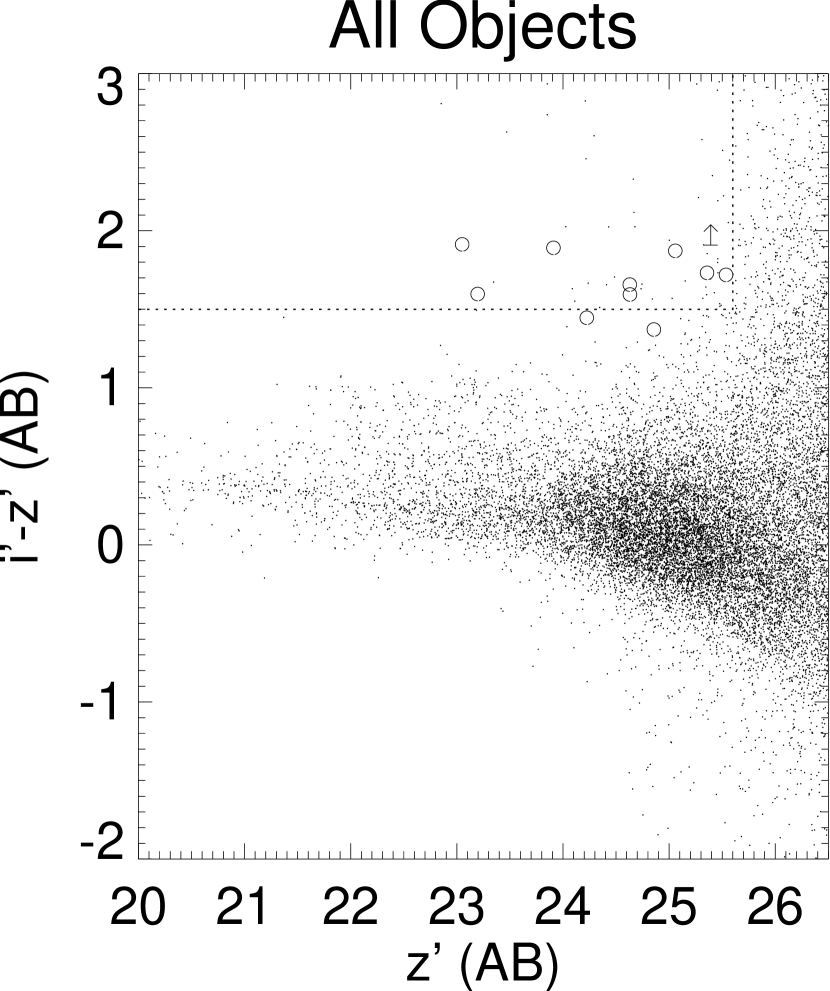
Figure 1.— Color selection of our candidates showing the $(i^{\prime}-z^{\prime})_{\rm AB}>1.5$, $z^{\prime}_{\rm AB}<25.6$ mag selection criteria applied in each epoch and indicating the colors of the candidate objects in table 1. A further two objects lying within $1\sigma$ our $i^{\prime}-z^{\prime}$ cut are included for completeness. Note that the catalog presented here is not clean and indicates the large number of data artifacts that can mimic these $i^{\prime}-z^{\prime}$ colours. A number of ‘objects’ identified in each epoch were in fact connected to unmasked satellite tracks or optical refraction artifacts and these objects were rejected from the final selections.

The fluxes of the remaining candidate objects were then measured directly within a 1″ diameter aperture in each epoch and these fluxes averaged to give a final magnitude, thereby reducing the photometric error for each object. To convert to total magnitudes, an aperture correction of 0.09 mag was applied to all objects, determined from aperture photometry of bright but unsaturated point sources. Although this correction will underestimate the magnitude of very extended sources, the candidate objects presented in this paper are all compact and it has not been necesary to apply different aperture corrections to different candidates.

Although a deeper candidate selection may have been possible using coadded images for selection, we have found that the advantages of being able to eliminate spurious and transient sources by epoch-epoch comparison are significant. An ideal algorithm for co-adding the images would reject all deviant pixels allowing identification of fainter objects, however such an algorithm is in practise difficult to obtain with just three or even five epochs of data and coadding the data here will lead to the loss of time-dependent information or information on poorly rejected spurious pixels. In several cases the time-averaged colour of an object was significantly affected by hot pixels or poorly rejected cosmic rays in a single epoch. The selection method outlined above allowed epochs for which the data were unreliable to be rejected when making a final selection. As a result we have chosen to work at a relatively bright magnitude limit on the shallower single epoch data. the completeness of our resulting sample is discused in section 4.

In table 1 we present details of the nine objects meeting our selection criteria. In addition the two objects which lie within $1\sigma$ of being selected are included in the following discussions for completeness. Postage stamp images of each object in the $v$, $i^{\prime}$, $z^{\prime}$ and $HK^{\prime}$ bands (see section 2.3) are presented in figure 2. None of the $i^{\prime}$-drops in table 1 were formally detected at $>3\sigma$ in the F606W ($v$) or F435W ($B$) band ($v_{AB}<27.3$, $B_{AB}<27.0$ mag) of GOODS/ACS observations except candidate 6 which may be subject to contamination from a nearby object (figure 2).

As illustrated by figure 3, 3 of the 9 $i^{\prime}$-drop objects in table 1 are unresolved in the GOODS/ACS $z^{\prime}$ images (R_h =0$\farcs$05). These objects may reasonably be Galactic stars, high redshift QSOs or compact galaxies. Previous studies have shown that galaxies at very high redshift are barely resolvable with HST (and are sometimes unresolved), examples including the $z>5$ candidates of Bremer et al. (2003) which have R${}_{h}\sim$0$\farcs$1-0$\farcs$3, and the barely-resolved spectroscopically confirmed z=5.78 galaxy SBM03#3 which has an R${}_{h}=$0$\farcs$08 (Paper 2). With this in mind, we consider each object individually rather than requiring that all galaxy candidates are resolved.

2.2. X-ray properties: Non-Detection of $i^{\prime}$-Drops by Chandra

To avoid possible contamination of our sample by high redshift AGN we examined publically-available deep data from the Chandra X-ray telescope.

All of our candidates lie in the region surveyed in a 2 Ms exposure by the Chandra X-ray satellite (Alexander et al. 2003) and none of these objects were detected by that survey, allowing us to place a limit on their X-ray fluxes $0.5-2$ keV (soft) and $2-8$ keV (hard) bands at between $1.9\times 10^{-17}$ and $9.3\times 10^{-17}$ ergs cm^-2 s^-1 and between $1.1\times 10^{-16}$ to $7.5\times 10^{-16}$ ergs cm^-2 s^-1 respectively, varying according to the non-uniform exposure across the GOODS-N field (D.M. Alexander, private communication). A powerful AGN (quasar) is expected to have a rest-frame 2-8 keV luminosity $>10^{44}\,h^{-2}_{70}\,{\rm erg\,s}^{-1}$ (Barger et al. 2003), which yields a flux at $z=5.8$ of $\sim 3\times 10^{-16}\,{\rm erg\,s}^{-1}\,{\rm cm}^{-2}$. Thus we would expect to detect X-ray luminous quasars for most of our sources at the relevant search redshifts probed in this paper.

This renders the identification of any of our candidates as powerful high-redshift AGN unlikely although non-detection of x-ray flux at these limits does not rule out the presence of fainter high redshift AGN such as those observed in $\approx 3\%$ of Lyman break galaxies at $z\sim 3$ (Steidel et al. 2002). In this $z\sim 3$ sample, AGN contribute less than 2% of the total rest-frame UV luminosity. Calculations in section 5 require an implicit assumption is that the rest-frame flux is dominated by star formation. Although an absence of luminous AGN does not necesarily imply a UV continuum dominated by star formation, it does decrease the likelihood of significantly non-stellar origins for the flux.

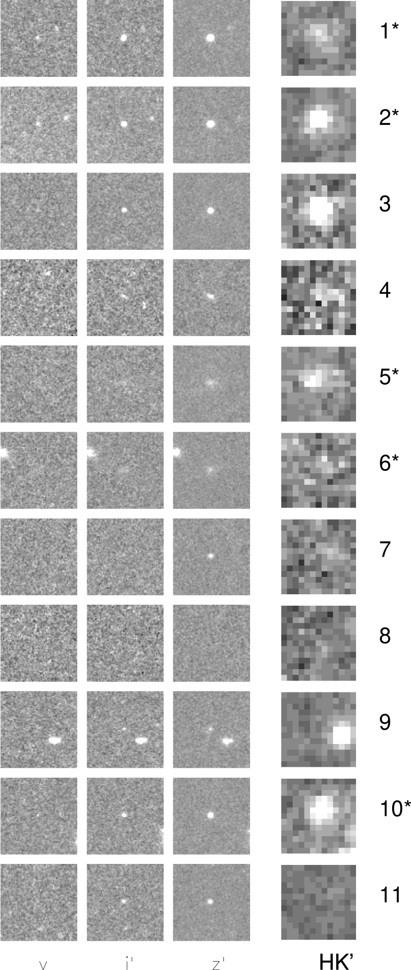
Figure 2.— $i^{\prime}$-drops in the GOODS-N field: HST/ACS and Hawaii $HK^{\prime}$, 4 arcsecond boxes. ACS images are constructed from all available epochs. An asterisk indicates that an object forms part of our spectroscopic sample.

Table 1$i^{\prime}$-drops in GOODS-N

ID	RA	Declination	$z^{\prime}_{\rm AB}$	$i^{\prime}_{\rm AB}$	$(i^{\prime}-z^{\prime})_{\rm AB}$	$(z^{\prime}-HK^{\prime})_{\rm AB}$	Rh	SFR${}^{z=5.8}_{\rm UV}$	Final
	(J2000)	(J2000)					arcsec	$h^{-2}_{70}\,M_{\odot}\,{\rm yr}^{-1}$	Cut?
$1$	12h36m58$\fs$13	+62°18′51$\farcs$5	$23.05\pm 0.02$	$24.96\pm 0.07$	$1.91\pm 0.07$	$0.21\pm 0.11$	$0.051$	[140]	No
$2$	12h37m34$\fs$04	+62°15′53$\farcs$4	$23.20\pm 0.02$	$24.79\pm 0.06$	$1.60\pm 0.06$	$1.62\pm 0.04$	$0.053$	[122]	No
$3$	12h36m38$\fs$85	+62°14′51$\farcs$9	$23.91\pm 0.04$	$25.80\pm 0.16$	$1.89\pm 0.17$	$1.89\pm 0.05$	$0.054$	[63]	No
$4$	12h35m37$\fs$21	+62°12′03$\farcs$5	$24.63\pm 0.07$	$26.13\pm 0.25$	$1.59\pm 0.26$	$<2.22$ $(2\,\sigma)$	$0.164$	33	Yes
$5$	12h36m48$\fs$47	+62°19′02$\farcs$0	$24.63\pm 0.07$	$26.29\pm 0.27$	$1.67\pm 0.28$	$1.70\pm 0.08$	$0.197$	33	Yes
$6$	12h37m39$\fs$29	+62°18′40$\farcs$2	$25.06\pm 0.10$	$26.93\pm 0.54$	$1.87\pm 0.55$	$<2.65$ $(2\,\sigma)$	$0.201$	22	Yes
$7$	12h35m52$\fs$35	+62°11′42$\farcs$1	$25.36\pm 0.14$	$27.09\pm 0.66$	$1.73\pm 0.67$	$<2.95$ $(2\,\sigma)$	$0.083$	17	Yes
$8$	12h36m50$\fs$41	+62°20′12$\farcs$6	$25.39\pm 0.14$	$<27.19$ $(2\,\sigma)$	$>1.71$ $(2\,\sigma)$	$<2.98$ $(2\,\sigma)$	$0.177$	16	Yes
$9$	12h36m48$\fs$74	+62°12′17$\farcs$1	$25.54\pm 0.16$	$<27.19$ $(2\,\sigma)$	$>1.56$ $(2\,\sigma)$	$<1.93$ $(2\,\sigma)$	$0.159$	14	Yes
$10$	12h36m53$\fs$79	+62°11′18$\farcs$2	$24.22\pm 0.05$	$25.67\pm 0.14$	$1.45\pm 0.15$	$1.96\pm 0.07$	$0.054$	[47]	No
$11$	12h36m49$\fs$79	+62°16′24$\farcs$9	$24.86\pm 0.09$	$26.23\pm 0.25$	$1.37\pm 0.26$	$<2.45$ $(2\,\sigma)$	$0.058$	[26]	No

Note. — Objects 10 and 11 (below the horizontal line) lie marginally outside our selection criteria but are included for completeness. All magnitudes are measured within a 1 arcsec diameter aperture. The half-light radius, $R_{h}$, is defined as the radius enclosing half the flux in the $z^{\prime}$ band. The nominal star formation rate (SFR) is calculated assuming objects are placed in the middle of our effective volume (a luminosity-weighted redshift of $z=5.8$) and are shown in square brackets if the candidate is not included in our final high redshift selection.

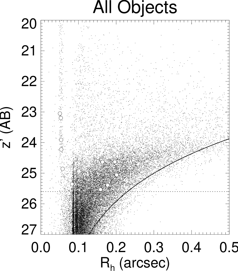
Figure 3.— The magnitude–size distribution of our GOODS-N $i$-drops (circles) and objects in the field. Note the cut-off at large half-light radii (R_h) due to surface brightness dimming (the solid curve is our completeness limit). Our magnitude limit is marked with a dotted line.

2.3. Near-infrared Imaging

As figure 4 illustrates, a color cut of $(i^{\prime}-z^{\prime})_{\rm AB}>1.5$ can be used to select galaxies with $z>5.6$. This color-cut criterion alone may also select elliptical galaxies at $z\simeq 2$ (e.g., Cimatti et al. 2002) and cool low-mass M/L/T stars (e.g., Kirkpatrick et al. 1999, Hawley et al. 2002). We can guard against such contaminants by utilizing near-infrared photometry. In particular the relatively blue $(z^{\prime}-HK^{\prime})>3$ color expected of $z\simeq 2$ ellipticals allows these objects to be distinguished from high redshift candidate objects.

In order to improve our discrimination between high and low redshift objects we have supplemented the GOODS HST/ACS data with publically-available near-infrared images from the Hawaii-HDFN project. The $HK^{\prime}$-band data is described in Capak et al. (2003), and was obtained on the University of Hawaii 2.2m telescope, with a pixel scale of $0\farcs 3\,{\rm pixel}^{-1}$. It covers an area of 0.11 deg² to a depth of $HK^{\prime}_{AB}=22.5$ (encompassing the entire GOODS area), with the central $9^{\prime}\times 9^{\prime}$ region imaged to a greater depth of $HK^{\prime}_{AB}=23.7$ ($2\,\sigma$, 1″ diameter aperture).

SExtractor was again used to identify objects in the $HK^{\prime}$ images with 5 or more adjacent pixels exceeding the background noise by 2$\sigma$. Matches for the $i^{\prime}$-drop candidate objects were assigned if positions of the sources were within $1\arcsec$, although we carefully examined the $z^{\prime}$-band image to see if nearby non-$i^{\prime}$-drop sources may instead be responsible for any near-infrared flux. An aperture correction of 0.4 mag was applied to the $1\arcsec$ aperture magnitudes in order to estimate the total flux.

Figure 4.— Evolutionary tracks and color discrimination: the solid black line indicates the evolutionary path followed by elliptical galaxies with redshift (calculated using the Coleman, Wu and Weedman (1980) spectral template). Also indicated by lines are evolutionary paths for Sab (dashed), Sbc (dotted) and Im (dot-dash) galaxies and for a Kinney et al. starburst model (dot-dot-dash). Tick marks on tracks indicate unit redshift intervals between $z=0$ (lower left) and $z=7$ (upper right). The vertical dotted line indicates our basic color-cut criterion of $(i^{\prime}-z^{\prime})_{\rm AB}>1.5$. The colors of candidates in table 1 are indicated with error bars or as upper limits in $(z^{\prime}-HK^{\prime})_{\rm AB}$. The colors of typical L class stars are shown as small diamonds, derived from the spectra from Reid et al. (2001).

Low redshift $z\simeq 1-2$ elliptical galaxies are known to be a contaminant in colour selected samples at $z>5$ (Capak et al. 2003, Bremer et al. 2003). Our $i^{\prime}-z^{\prime}$ colour cut criterion was designed to exclude these but contamination is still possible due to scatter in the photometric properties of these objects. Although the near infrared colors of many of the objects presented in table 1, as shown on figure 4, are presented only as upper limits, those limits all place $(z^{\prime}-HK^{\prime})_{\rm AB}<2.5$ with the exception of those for candidates 7 and 8. Given the red $(i^{\prime}-z^{\prime})_{\rm AB}$ colour of candidate 8, only candidate 7 is marginally consistent with being a low redshift elliptical galaxy. The lower limit of $(z^{\prime}-HK^{\prime})_{\rm AB}<2.95$ for this object, however, does not preclude the possibility that candidate 7 may also lie at much higher redshift.

The region of colour space occupied by L and M class stars is less clearly distinct from that occupied by high redshift galaxies. Four objects (candidates 2, 3, 5 and 10) have colors consistent with identification as L class stars although all four are also still consistant with a high redshift interpretation if the spectral slope of high redshift objects is steeper than that observed in $z\sim 3$ LBGs. Candidate 1 has colours which are consistant with either a high redshift galaxy or a mid-M class star. Near-IR colours, together with their spectroscopy and other properties, are considered in section 3.2 where a final high redshift candidate selection is made.

3. $I$-Drops – SPECTROSCOPIC PROPERTIES FOR THE HDF NORTH AND CDF SOUTH SAMPLES

3.1. Spectroscopy - Observation Data

We have obtained slit-mask spectra of about half our $i^{\prime}$-drop sample, using the Deep Imaging Multi-Object Spectrograph (DEIMOS, Faber et al. 2002; Phillips et al. 2002) at the Cassegrain focus of the 10-m Keck II Telescope. DEIMOS has 8 MIT/LL $2k\times 4k$ CCDs with $15\,\mu$m pixels and an angular pixel scale of 0.1185 arcsec pix^-1. The seeing was typically in the range $0\farcs 7-1\farcs 0$ FWHM, smaller than or comparable to the slit width of $1\farcs 0$.

The observations were obtained using the Gold 1200 line mm^-1 grating in first order. The grating was tilted to place a central wavelength of 8000 Å on the detectors, and produce a dispersion of $0.314$ Å pixel^-1. We sample a wavelength range of approximately $\lambda\lambda_{\rm obs}\,6600-9100$ Å, corresponding to a rest-frame wavelength of $\lambda\lambda_{\rm rest}\,950-1300$ Å at $z\sim 6$. Wavelength calibration was obtained from Ne$+$Ar$+$Hg$+$Kr reference arc lamps. The spectral resolution was measured to be $\Delta\lambda_{\rm FWHM}^{obs}\approx 1.4$ Å ($\Delta v_{\rm FWHM}\approx 55$ km s^-1) from the sky lines. A small 8 Å region in the middle of the wavelength range for each object is unobserved as it falls in the gap between two CCDs. The fraction of the spectrum affected by skylines is small ($<2$ per cent). Flux calibration was determined using the spectra of the alignment stars of known broad-band photometry ($I\approx 16-19$ mag), used to position the two slitmasks through $2^{\prime\prime}\times 2^{\prime\prime}$ alignment boxes.

In Paper 2 we already reported the confirmation of a $z=5.8$ galaxy (SBM03#3 in GOODS-S from Paper 1), based on a 5.5-hour DEIMOS spectrum taken on UT 2003 January 08 & 09. In section 3.3 we present spectra from other GOODS-S $i^{\prime}$-drops on the same slitmask. Our spectroscopy reveals a second $z=5.8$ Lyman-$\alpha$ emitter in the same field. The observations and data reduction for this slitmask are as detailed in paper 2.

In addition, we have recently obtained ultra-deep spectroscopy of our GOODS-N $i^{\prime}$-drops over the 5 nights of U.T. 2003 April 2-6. We used several slitmasks to target a subset of five of the eleven objects in table 1 (candidates 1, 2, 5, 6 and 10). The $i^{\prime}$-drops were placed on slitmasks for a primary program targetting $z\simeq 1$ E/S0 galaxies in the GOODS-N field (Treu et al. in prep). The selection of $i^{\prime}$-drops from table 1 for the masks was purely geometric and accordingly randomized. The position angle of slits on the mask was chosen to be 45.3° so as to align the large ($16.5\times 5$ arcmin) DEIMOS field of view with the axis of the GOODS-N HST/ACS observations. The spectra were pipeline reduced using version 1.1.3 of the DEEP2 DEIMOS data reduction software.

A total of 37.8 ksec (10.5-hours) of on-source integration was obtained in each of three slitmasks, and this was broken into individual exposures each of duration 1800 s. These spectra are therefore a factor of $\sqrt{2}$ deeper than the 5.5-hour spectra of GOODS-S introduced in paper 2. In 10.5 hours of DEIMOS spectroscopy we reach a flux limit of $2\times 10^{-18}\,{\rm ergs\,cm}^{-1}\,{\rm s}^{-1}$ ($5\,\sigma$) for an emission line uncontaminated by sky lines and extracted over 8Å (300 km s^-1) and 1″.

The results of this spectroscopy are summarised in table 2 and discussed in more detail in the following sections.

Table 2Summary of Spectroscopic Results

Object	Observation
GOODS-S SBM03#1*	Line emission at 8305Å - identified as Lyman-$\alpha$
GOODS-S SBM03#2	No observed spectral features
GOODS-S SBM03#3*	Line emission at 8245Å - identified as Lyman-$\alpha$
GOODS-S SBM03#5	No observed spectral features
GOODS-S SBM03#7*	No observed spectral features
GOODS-N#1	Continuum Flux longward of approx. 7200Å
GOODS-N#2	Continuum Flux longward of approx. 7800Å
GOODS-N#5*	No observed spectral features
GOODS-N#6*	Line emission at 8804Å - identification uncertain
GOODS-N#10	No observed spectral features

Note. — Objects identified as high redshift candidates are marked with an asterisk.

3.2. GOODS-North Candidate Spectra and Final Selection

Since all the objects presented in table 1 satisfy our primary $i^{\prime}-z^{\prime}$ color selection criterion and do not have $z^{\prime}-HK^{\prime}$ colors indicative of being lower redshift elliptical galaxies, our most significant remaining source of contamination in a high redshift sample is likely to be cool galactic stars. These constitute two of the nine $i$-drop objects in the GOODS-S field (paper 1) and are often excluded from colour selected samples by the simple expedient of rejecting all unresolved sources (e.g. Bouwens et al. 2003). In this section we consider the interpretation of the candidate spectra for those objects for which such is available, the probable classification of each candidate in table 1 and the construction of a robust sample of high redshift galaxies.

Five objects in GOODS-N were targeted for spectroscopic observations. Two yielded continuum detections, and a likely identification as cold stars (candidates 1 and 2). One spectrum (candidate 6) shows a single extended emission line feature at 8804 Å, with the peak emission spatially offset from the continuum location by $\sim 2\arcsec$ (and hence this spectral feature may be associated with an adjacent foreground object). No signal was detected in the other two spectra (candidates 5 and 10). A description of each spectrum follows.

3.2.1 GOODS-N $i^{\prime}$-Drop #1

The spectrum of GOODS-N $i^{\prime}$-drop #1 does not appear to show any distinctive emission lines. The object continuum, however, is clearly detected at long wavelengths. Figure 5 presents a box-car smoothed spectrum of this object together with the spectrum of an L-class star (2MJ0345432+254023, class L0 for comparison.

The object’s spectrum and compactness R_h =0$\farcs$05 (unresolved) are both strongly suggestive that this object may be identified as an M or early L class star and although the spectrum obtained has very low signal-to-noise, there are suggestive commonalities with the L0 spectrum such as the absorption feature at $\sim$8400Å. In addition its colors are marginally consistent with identification as a mid M-class star, although the near-infrared colors are affected by a near neighbor. We provisionally identify this unresolved source as a galactic star, and hence exclude it from our final high redshift sample.

3.2.2 GOODS-N $i^{\prime}$-Drop #2

As in the case of GOODS-N $i^{\prime}$-drop #1, the spectrum of GOODS-N $i^{\prime}$-drop #2 does not appear to show any distinctive emission lines but the object continuum is clearly detected at long wavelengths. Figure 5 presents a smoothed spectrum of this object. Both the continuum colors of this object and its compactness (R_h =0$\farcs$05, unresolved) suggest that this object may be an L dwarf star, although it lacks the absorption at $\sim$8400Å often seen in L class stars. The low signal-to-noise spectrum of this object shows a moderate cross correlation with those of L class stars and a weaker correlation with the composite LBG spectrum of Shapley et al. (2003), redshifted to $z\sim 6$. We tentatively identify this object as a cool galactic star and it is therefore excluded from our final list of good high redshift candidates. As the classification of this object is uncertain it should be noted that, as one of the brighter objects selected by our $(i^{\prime}-z^{\prime})_{\rm AB}$ color criterion, this object would have a significant effect on our calculations in section 5 if it was shown to lie at high redshift, as is discussed in that section.

Figure 5.— GOODS-N $i^{\prime}$-drops #1 and #2 — Spectra are binned into 10 Å bins (33 pixels) and are extracted over 1″ (9 pixels). The spectrum of candidate 2 is offset by $2\times 10^{-18}\,\mathrm{ergs\,cm}^{-2}\,\mathrm{s}^{-1}$ for clarity. The spectrum of the L0 Dwarf star 2MJ0345432+254023 (2MASS, Reid et al. 1999) is plotted for comparison (offest by $1\times 10^{-18}\,\mathrm{ergs\,cm}^{-2}\,\mathrm{s}^{-1}$), along with the sky spectrum (both with arbitrary scaling). The primary spectral features of L class stars are marked with arrows and correspond to the following lines respectively: TiO, TiO, K i, K i, Rb i, Rb i, Na i, Na i, TiO, TiO, CS i (Kirkpatrick et al. 1999).

3.2.3 GOODS-N $i^{\prime}$-Drop #5

Although a spectrum was obtained for GOODS-N $i^{\prime}$-drop #5, no spectral features or continuum flux were observed. However this object is relatively faint ($z^{\prime}_{\rm AB}=24.6$) and so we would be unlikely to detect continuum emission. Our limit on the equivalent width of an emission line is $W_{obs}<10$ Å (5 $\sigma$, 300 km s^-1 width), provided it lies away from a sky line. GOODS-N $i^{\prime}$-drop #5 is relatively extended and so unlikely to be a galactic star. Its near-infrared color is also inconsistent with identification as an elliptical galaxy at $z\sim 2$ although the colors are not fully consistent with a high redshift identification either. We include candidate 5 in our list of high redshift candidates although we note the ambiguity in its near-infrared colors.

3.2.4 GOODS-N $i^{\prime}$-Drop #6

The 2D spectrum of GOODS-N $i^{\prime}$-drop #6 showed one significant emission line detected at $\approx 20\,\sigma$ at a central wavelength of $\lambda_{\rm obs}\sim 8804\pm 1$ Å. Both 2D and 1D extracted spectra for this line are shown in figure 6, centered on the spatial location of the $i^{\prime}$-drop object and the central wavelength of the emission line. The emission line is spatially extended, stretching from the location of the $i^{\prime}$-drop in the ACS imaging to peak in intensity approximately $2\arcsec$ away .

The line flux is $(7\pm 2)\times 10^{-18}\,\mathrm{ergs\,cm}^{-2}\,\mathrm{s}^{-1}$ measured between the zero power points at 8798.0Å and 8813.5Å in an extraction width of $3\arcsec$ centered on the peak of the line emission. As figure 6 shows, the line profile is clearly resolved and shows velocity structure, although it is not obviously a doublet. The FWHM of the emission line is $(10.0\pm 1.0)$Å although the central peak of emission is narrower with a FWHM of $(4.0\pm 0.25)$Å.

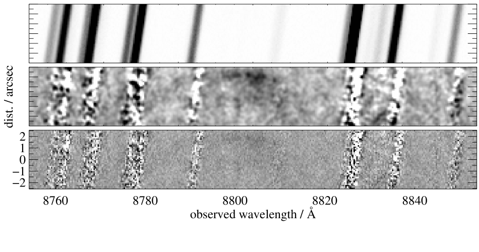
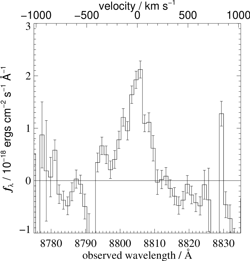
Figure 6.— (a) GOODS-N $i^{\prime}$-drop #6 2D spectrum — Candidate Lyman-$\alpha$ emission line at $z=6.24$ (lower panel), sky spectrum (upper panel), 2D spectrum boxcar smoothed over 3 pixel resolution elements (centre panel). The 2D spectra span a spatial range of $\pm 2.5\arcsec$ around the $i^{\prime}$-drop location on slit. The emission line is centered 1$\farcs$5 from the candidate object but extends to its location. (Right) HST/ACS image showing the slit orientation. Box length is 10″. As can be seen the neighbouring object lies just off the slit but some flux from this neighbour would be expected to fall down the slit in ground-based seeing. (b) The 1D spectrum extracted over 2″ around the emission line center, and binned into independent spectral resolution elements of 1.2 Å (4 pixels). The features around 8790 Å and 8830 Å are sky-subtraction residuals.

GOODS-N $i^{\prime}$-drop #6 is a relatively extended, faint galaxy with a brighter neighbor at approximately $2\arcsec$ separation along the slit direction. The neighboring object is expected to lie just off the slit, although given the seeing conditions of this observation ($\sim 0\farcs 8$) we may expect some light from this object to fall into our slit near the location of the emission line. As a result we suggest two possible interpretations of this observation.

One possible scenario is that the line emission is associated with this lower-redshift (non-$i^{\prime}$-drop) neighboring galaxy. The observed line is isolated, with no other lines detected. The neighbor has a photometric redshift of $z=2.605\pm 0.2$, based on its colors in the GOODS/ACS imaging and determined using the template fitting routine ‘HyperZ’ (Bolzonella et al. 2000). The observed line cannot be easily identified with any emission line at $z=2.6$ ($\lambda_{\rm rest}\sim 2442$Å). It is inconsistent with identification as a $z=1.36$ [O ii] ($\lambda_{\rm rest}=3726,3729$Å), and no doublet structure is obvious, although the line could conceivably be Mg ii ($\lambda_{\rm rest}\sim 2795$Å) at $z=2.15$.

The second scenario is that we are seeing spatially-extended Lyman-$\alpha$ emission at $z=6.24$, as has been observed in a number of star forming galaxies. Observations of a lensed $z=4$ galaxy by Bunker et al. (2000) identified Ly-$\alpha$ emission offset by 1-2″ from the rest frame UV continuum region (although this corresponds to only 0.7$\,h_{70}^{-1}\,$kpc at $z=4$ given the lensing amplification of $\sim 10$ for this galaxy). Similarly, Steidel and coworkers (2000) identify two Lyman-$\alpha$ ‘blobs’ associated with but not centered on continuum emission Lyman break galaxies at $z\sim 3$. These Lyman-$\alpha$ regions extend over $>100\,h_{70}^{-1}\,$kpc and are similar to extended Lyman-$\alpha$ emission seen in the vicinity of high redshift radio-galaxies.

At $z\sim 6$ a spatial offset of 2 ″ corresponds to a physical separation of $11.4\,h^{-1}_{70}$ kpc, larger than that observed in the $z=4$ galaxy but much smaller than the extended Lyman-$\alpha$ observed by Steidel et al. (2000). If we identify the emission line as Lyman-$\alpha$ then the emission wavelength is $\lambda_{\rm rest}\sim 1216$Å giving a redshift for candidate 6 of $z=6.24$. We tentatively adopt this identification and candidate 6 remains part of our high redshift galaxy sample.

3.2.5 GOODS-N $i^{\prime}$-Drop #10

GOODS-N $i^{\prime}$-drop #10 was selected with marginal $i^{\prime}-z^{\prime}$ colors, slightly below our strict color cut criterion. The spectra of this object shows no significant features or continuum flux in its spectrum. Both its compact (unresolved) $R_{h}$ and $(z^{\prime}-HK^{\prime})_{\rm AB}$ color suggests that this may be a low mass star. Given that this object did not meet our strict criteria, the relative brightness and its lack of strong high redshift emission features we exclude this object from our final selection as a probable low mass star although, again, we consider the effects of including this object in section 5.

3.2.6 GOODS-N $i^{\prime}$-Drops for Which No Spectra Are Available

In common with GOODS-N $i^{\prime}$-drops #2 and #10, GOODS-N $i^{\prime}$-drop #3 is unresolved and its $z^{\prime}-HK^{\prime}$ color is completely consistent with identification as an L-class dwarf star (Reid et al. 2001). It is thus excluded from the final robust high redshift sample although the effects of including all our stellar candidates as possible high redshift objects is discussed in section 5.

GOODS-N $i^{\prime}$-drops #4 and #8, on the other hand, are relatively extended objects and so are inconsistent with identification as galactic stars. Their near-infrared colors are also inconsistent with elliptical galaxies at $z\sim 2$ suggesting that they may safely be identified as high redshift candidates. These candidates remain in our selection.

GOODS-N $i^{\prime}$-drop #9 is relatively extended and can be identified with Fernández-Soto, Lanzetta and Yahil (1999) object 311 which was given a photometric redshift of $z_{\rm phot}=5.64$ by those authors, consistent with our result. This is the only high-redshift candidate object here to appear in the Fernández-Soto, Lanzetta and Yahil (1999) photometric redshift catalogue for the HDFN. Since GOODS-N $i^{\prime}$-drop #9 is inside the central Hubble Deep Field North region, it is observed in deep NICMOS near-infrared imaging (Thompson et al. 1999), as shown in figure 7, from which we have obtained this object’s near infrared magnitudes in the F110W${}_{\rm AB}(J)$ and F160W${}_{\rm AB}(H)$ bands. Its colors of $(z^{\prime}-J)_{\rm AB}\sim 0.53$ and $(J-H)_{\rm AB}\sim 0.50$ are consistent with a high redshift interpretation and inconsistent with the colors of low redshift galaxies. As a result we include it in our list of final candidates.

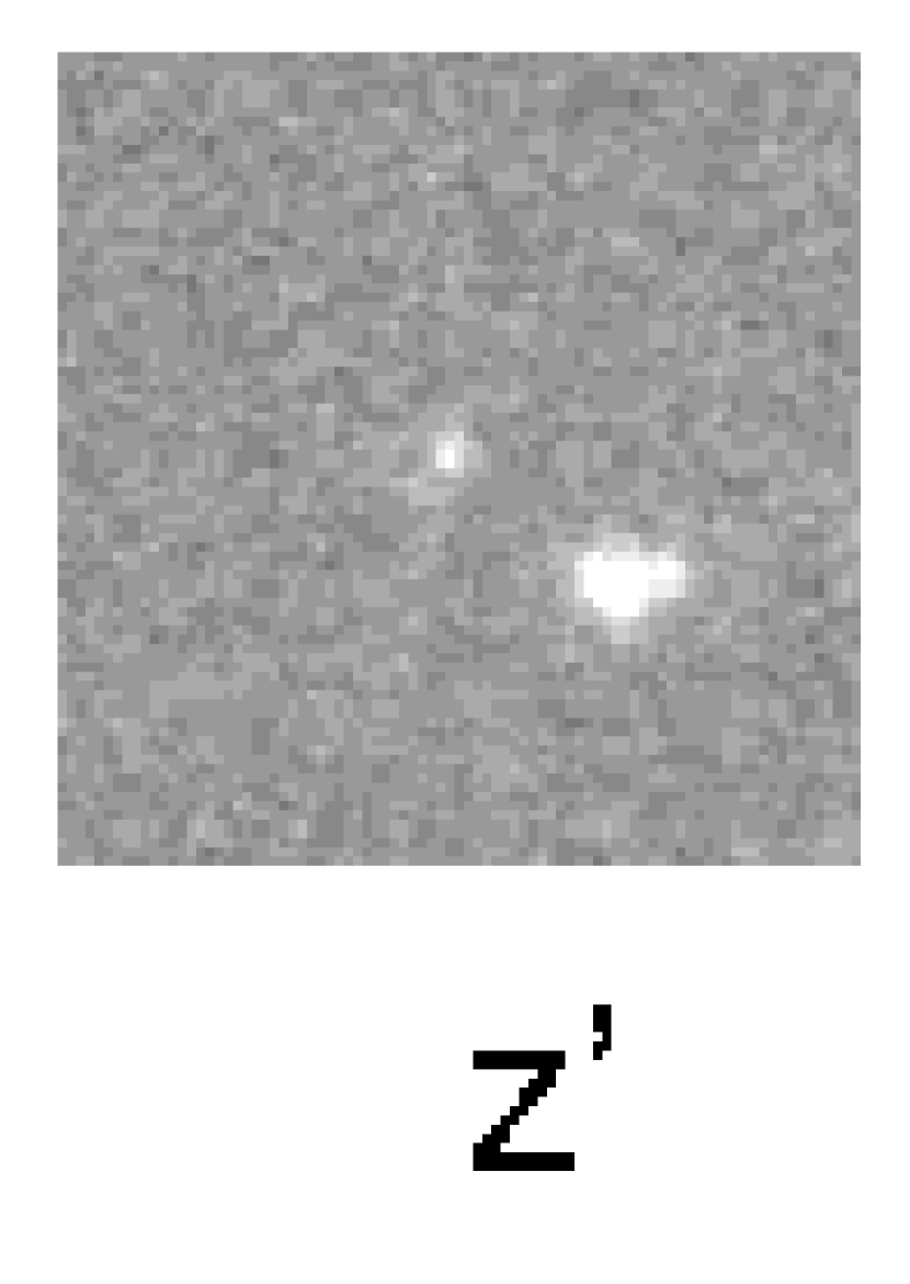
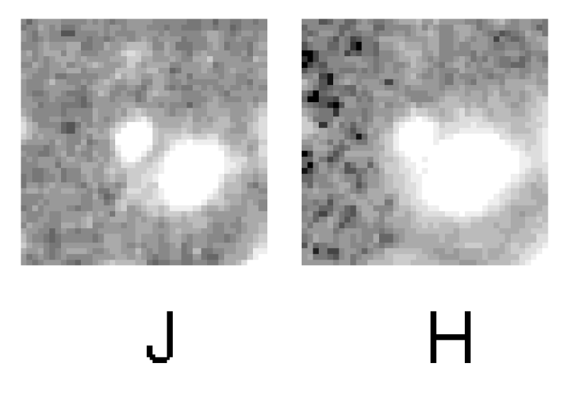
Figure 7.— GOODS-N $i^{\prime}$-drop #9 in the ACS $z^{\prime}$-band image and in the NICMOS F110W${}_{\rm AB}(J)$ and F160W${}_{\rm AB}(H)$ imaging of the Hubble Deep Field North.

Since GOODS-N $i^{\prime}$-drop #11 was selected with marginal $(i^{\prime}-z^{\prime})_{\rm AB}$ colors, not meeting the strict $(i^{\prime}-z^{\prime})_{\rm AB}<1.5$ color cut, and is also unresolved it has also been rejected as a probable low mass star despite the lack of a strong near-infrared color constraint. This is the only object excluded from our final candidate selection primarily on grounds of its unresolved nature. As such we note that its inclusion in our final selection would have increased the observed star formation rate of that sample by 18% (see section 5).

3.3. Spectroscopy of $i^{\prime}$-drops in GOODS-South Field

3.3.1 GOODS-S SBM03#1

Our 5.5-hour spectrum of GOODS-S $i^{\prime}$-drop #1 in paper 1 (hereafter SBM03#1) reveals a single emission line at $8305.3\pm 0.9$ Å at the same location on the 1″-wide longslit as the $i^{\prime}$-drop ($\alpha_{2000}=03^{h}32^{m}40.0^{s}$, $\delta_{2000}=-27^{\circ}48^{\prime}15.0^{\prime\prime}$). The emission line falls between two sky lines, and the 2D spectrum is shown in figure 8.

The spectrum is very similar to that of GOODS-S SBM03#3 reported in Paper 2, where we argued that the most likely interpretation of the solo emission line at 8245 Å was Lyman-$\alpha$ at $z=5.78$, given the $i^{\prime}$-drop selection and the fact that we would resolve the [OII] doublet at lower redshift (and most other prominent emission lines would have neighboring lines within our wavelength range). Applying the same logic to our spectrum of GOODS-S SBM03#1, it seems likely that the emission line is Lyman-$\alpha$ at $z=5.83$ – a view supported by the characteristic asymmetry in the emission line spectrum, with a sharp blue-wing cut-off. The redshift of SBM03#1 is very close to the redshift of SBM03#3 (the line centers are separated by 2000 km s^-1), and the spatial separation of 8 arcmin corresponds to a projected separation of only $2.9\,h_{70}^{-1}$ Mpc.

The flux in this emission line is comparable to that of SBM03#3 at $z=5.78$, and is within 30 per cent of $f=2\times 10^{-17}\,{\rm erg\,cm^{-2}\,s^{-1}}$, extracting over 17pixels (2 arcsec) and measuring between the zero-power points ($8300-8318$ Å). This is a lower limit due to potential slit losses, although these are likely to be small, since like SBM03#3, SBM03#1 is compact ($R_{\rm hl}=0.1\arcsec$, paper 1). After deconvolving with the ACS $z^{\prime}$-band point spread function, the half-light radius corresponds to a physical size of only $0.5\,h^{-1}_{70}$ kpc.

In continuum, SBM03#1 is half the brightness of SBM03# (paper 2) from the $z^{\prime}$-band magnitude. The equivalent width is $W_{\rm rest}^{\rm Ly\alpha}=30\pm 10$ Å, at the upper end of the distribution observed in $z=3-4$ Lyman break galaxies (Steidel et al. 1999). The star formation rate from the rest-frame UV continuum is $17\,h^{-2}_{70}\,M_{\odot}\,{\rm yr}^{-1}$ (paper 1).

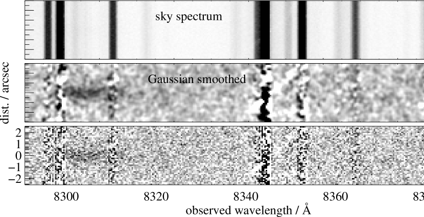
Figure 8.— (a) The lower panel shows the two-dimensional spectrum of GOODS-S SBM03#1 (candidate 1 in paper 1) around Lyman-$\alpha$ (100 Å by 5 arcsec), the middle panel shows this smoothed with a Gaussian of $\sigma=1$ pixel, and the upper panel shows the sky spectrum for this range. The line is centered at 8305 Å. (b) The one-dimensional spectrum of SBM03#1 around Lyman-$\alpha$, extracted over a 9pixel (1 aecsec) width. The data have been binned into independent spectral resolution elements of 1.3 Å (4 pixels).

3.3.2 Further Candidates in GOODS-S

As described in Paper 2, DEIMOS spectroscopy of three further candidates (SBM03#2,5,7) was obtained with the Keck II telescope. Inspection of these spectra reveals no obvious Lyman $\alpha$ emission or continuum emission within the wavelength range sampled. At present the nature of these sources is unfortunately unclear.

4. High Redshift Galaxies - Derived Parameters and Interpretation

4.1. Survey Volume and Completeness

Galaxies in the redshift range $5.6<z<7.0$ are selected by our color-cut provided they are sufficiently luminous. However, as we discuss in paper 1, our sensitivity to star formation is not uniform over our survey volume: at higher redshifts, we are only sensitive to more luminous galaxies at our apparent magnitude limit of $z^{\prime}_{AB}=25.6$, exacerbated by the increasing fraction of the $z^{\prime}$-band extincted by the Lyman-$\alpha$ forest, and there is a $k$-correction as we sample progressively shorter rest-frame wavelengths. As a result of this luminosity bias, the average redshift of objects satisfying our selection criteria is towards the lower end of the redshift range above and we calculate this luminosity-weighted central redshift as $z=5.8$ under the assumption of no evolution in the luminosity function from that at $z\sim 3$. In paper 1 we followed the methodology of Steidel et al. (1999) to quantify the incompleteness due to luminosity bias with redshift by calculating the effective volume of the survey. If there is no change in $L^{*}_{LBG}$(1500 Å) or $\alpha$ from $z=3$ to $z\approx 6$ (i.e. no evolution in the galaxy luminosity function from that of Steidel et al. 1999 at $z=3$), we showed that for our ACS $z^{\prime}$-band limit for the GOODS data, the effective volume is 40 per cent that of the total volume in the interval $5.6<z<7.0$. For our 200 arcmin² survey area (including areas only surveyed in half of the epochs and after excluding the unreliable regions close to the CCD chip gaps) this corresponds to an effective comoving volume of $V_{\rm eff}=2.5\times 10^{5}\,h^{-3}_{70}\,{\rm Mpc}^{3}$. This assumes a spectrum flat in $f_{\nu}$ at wavelengths longward of Lyman-$\alpha$ (i.e., $f_{\lambda}\propto\lambda^{-\beta}$ where $\beta=2.0$). For a redder spectrum with $\beta=1.1$ (the mean reddening of the $z\approx 3$ Lyman break galaxies, Meurer et al. 1997) the effective volume is 36 per cent of the total ($V_{\rm eff}=2.3\times 10^{5}\,h^{-3}_{70}\,{\rm Mpc}^{3}$ comoving) – which would result in an 8% rise in the measured star formation density (section 5) compared with $\beta=2.0$.

The above discussion, however does not take into account the effects of survey incompleteness due to photometric scatter, extreme intrinsic color variation or cosmological surface brightness dimming.

Our selection procedure is robust to the effects of photometric scatter. By utilizing four epochs of data and selecting objects in each which satisfy our criteria, only those objects lying more than 1$\sigma$ from their true magnitudes in four independent measurements will be entirely missed (fewer than 1% of the population assuming Gaussian errors on the magnitudes). It is possible, however, that the effects of photometric errors in one or more epochs may sufficiently affect the combined flux of the observations to take an object below our $(i^{\prime}-z^{\prime})_{\rm AB}$ selection limit. In practise only two objects in our epoch-by-epoch selection sub-catalogue showed $(i^{\prime}-z^{\prime})_{\rm AB}$ colors that consistantly exceeded $(i^{\prime}-z^{\prime})_{\rm AB}>1.3$ and fluctuated around our color cut and these were included in table 1 as candidates 10 and 11. Both these objects were excluded from the final high redshift candidate selection on the basis of their stellar colors and full-width half-maxima. Since relaxing our colour cut criterion to $(i^{\prime}-z^{\prime})_{\rm AB}>1.3$ does not significantly add to the number of candidate objects, while at the same time increasing the likely fraction of low redshift contaminants (see figure 4), we estimate that the fraction of objects falling out of our selection due to photometric errors is small.

The effect of extreme scatter in the distribution of intrinsic object colors on the completeness of our selection is difficult to quantify given the unknown nature of the $z\sim 6$ population. Our color selection criterion illustrated in figure 4 is based upon the colors predicted by the evolution of empirical galaxy templates. This procedure has been shown to work well in the selection of Lyman break galaxies at $z\sim 3-4$ but does not account for atypical galaxies or for any significant deviation in the spectral shape of very high redshift objects from the templates.

As described in section 2, simulations were made to assess the completeness of our $i^{\prime}-z^{\prime}$ colour selection criterion on a galaxy population with the characteristics of the $z\sim 3$ Lyman break galaxies (Adelberger & Steidel 2000). These found that $>99$% of $z\geq 5.7$ galaxies brighter than our luminosity limit in such a population would be identified using this technique, with a somewhat lower completeness in the $5.6<z<5.7$ redshift bin where the completeness depends sensitively on the filter transmission and the model of IGM absorption. Relaxing the colour cut criterion to $(i^{\prime}-z^{\prime})_{\rm AB}>1.3$ would increase our completeness in the $5.6<z<5.7$ redshift bin by $\approx 10\%$ without affecting completeness in the higher redshift bins but, as noted above, would also slightly increase the levels of contamination from $z\sim 2$ elliptical galaxies.

The characteristics of the $z\sim 6$ population are currently unknown with neither the luminosity function or the distribution of spectral slopes accessible to the available data and it is possible that there is significant evolution in these properties in the interval $3<z<6$. However, the $i^{\prime}-z^{\prime}$ colour of galaxies at these high redshifts is driven primarily by the break caused by absorption in the intervening intergalactic medium. As a result the $i^{\prime}-z^{\prime}$ colour is effectively independent of spectral slope and the colours of a wide variety of intrinsic spectral energy distributions converge for $z>5$.

The single object confirmed to lie within our redshift range in the GOODS-N field (HDF 4-473 at $z=5.60$, Weymann et al. 1998) is slightly too faint to appear in our object selection ($z^{\prime}_{\rm AB}=26.66$, Bouwens et al. 2003a). More significantly, this galaxy is also too blue to appear in our selection ($(i^{\prime}-z^{\prime})_{\rm AB}=1.2$, Bouwens et al. 2003a), having been observed as a $V$ band drop-out, and so raises the possibility that we are excluding real objects by applying our color-cut. We note that HDF 4-473 is at the very lower end of the redshift range to which we are sensitive, and hence in a bin where our completeness is relatively poor. Nonetheless this object highlights the caution which must be applied to the interpretation of any sample selected purely on photometric criteria.

4.2. Physical Sizes of the $i^{\prime}$-drops and Surface Brightness Selection Effects

Our final catalog selection includes objects with observed sizes in the range R${}_{h}\sim 0\farcs 08-0\farcs 20$, similar to the observed range of sizes in the 6 $z\sim 6$ candidates we presented in paper 1. This range corresponds to projected physical sizes of $0.3-1.0\,h^{-1}_{70}\,$kpc at $z\sim 5.8$, deconvolved with the instrument PSF. The size range of our total sample of 12 $z\sim 6$ objects (paper 1 + this work) is comparable to, or smaller than, those of $z>5$ galaxies reported by Bremer et al. (2003). Bremer and coworkers identified a sample of 44 sources with half-light radii of R${}_{h}\sim 0\farcs 1-0\farcs 3$ and suggested that, when taken in conjunction with observations at lower redshifts, their results implied a modest decrease in galaxy scale lengths with redshift. Our results appear to support this conclusion, although it should be noted that at $z^{\prime}_{\rm AB}=25.6$, objects more extended than R${}_{h}\sim 0\farcs 25$ ($1.5\,h^{-1}_{70}\,$kpc) fall out of our selection due to low surface brightness (as shown in figure 3), thus placing a significant observational selection effect on the observed distribution of sizes.

Simulations were performed using the IRAF.Artdata package, placing artificial galaxies in the GOODS images in order to test the recoverability of such objects given our SExtractor detection parameters. We model the input population as having exponential disk surface brightness profiles with half light radii distributed uniformly between the instrumental point spread function (0$\farcs$05) and 0$\farcs$5. We find that we reliably recover $>$95% of the input galaxies for half-light radii R${}_{h}<0\farcs 25$ and $>$98% of galaxies with R${}_{h}\sim 0\farcs 20$ with the remaining 2% being lost because of crowding.

Nonetheless, at brighter magnitudes our objects do not occupy the full range of half-light radii allowed by the observational constraint: at $z^{\prime}_{\rm AB}=24.7$ (the magnitude of our brightest high redshift candidate) we are sensitive to objects as large as R${}_{h}\sim 0\farcs 34$ (see figure 3). This suggests that most objects at high redshift are small enough to fall within our surface brightness selection limit.

Star forming regions in the local universe are often very compact in the UV continuum and it is likely that this is also true at high redshift. Lowenthal et al. (1997) report that Lyman break galaxies at $z\sim 3$ are compact and, if projected to $z\sim 3$, this population would range in half-light radius from 0$\farcs$08-0$\farcs$35 with a median size of R${}_{h}=0\farcs 18$. Although just over half of this range of half-light radii would be detectable at our magnitude limit, the full range of half-light radii are accessible to this sample at brighter magnitudes and failure to detect such objects may indicate a reduction in the physical scale of galaxies with increasing redshift. At $z>5$ Bremer and coworkers (2003) identified only 2 candidate objects on scales significantly larger than R${}_{h}\sim 0\farcs 3$ ($1.8\,h^{-2}_{70}$  kpc at $z\sim 5.2$) in a sample of 44 galaxies and considered these objects most likely to be $z\sim 1$ red galaxies. Iwata et al. (2003) made a similar selection of Lyman break galaxies at $z>5$ and found 40 per cent of their candidate objects were unresolved although they were limited by seeing conditions in their ground based observations. As Bremer et al. discuss, they expect a contamination from lower redshift galaxies of $\sim 20\%$ in their sample and also expect such objects to be resolved on scales of $>0\farcs 3$.

While this constraint on the physical size of observed objects is not explicitly accounted for in our effective volume calculation, the change in the angular diameter of objects of the same physical size over our redshift range is only 10 per cent. Given the evidence for a slight reduction in intrinsic object size with redshift (Bremer et al. 2003, Roche et al. 1998), and the failure of our candidates to occupy the full size range allowed by our observations even at fainter magnitudes, we expect the fraction of objects lost due to surface brightness effects to be small ($<2$%) and the effect on our effective survey volume to be negligible.

5. The Star Formation Rate at $z\sim 6$

5.1. The Global Star Formation History in GOODS-N

Since the primary sources of rest-frame ultraviolet photons within a galaxy are short-lived massive stars, UV flux is a tracer of star formation and its rest-frame UV flux density can be used to quantify the total star formation rate (SFR) within a galaxy. This rest-frame ultraviolet continuum is measured at $z\sim 6$ by the $z^{\prime}$ photometric band.

The relation between the flux density in the rest-UV around $\approx 1500$ Å and the star formation rate (${\rm SFR}$ in $M_{\odot}\,{\rm yr}^{-1}$) is usually assumed to be given by $L_{\rm UV}=8\times 10^{27}{\rm SFR}\,{\rm ergs\,s^{-1}\,Hz^{-1}}$ (Madau, Pozzetti & Dickinson 1998) for a Salpeter (1955) stellar initial mass function (IMF) with $0.1\,M_{\odot}<M^{*}<125\,M_{\odot}$.

Our limiting star formation rate as a function of redshift was considered in detail in paper 1, section 4 and illustrated in figure 6 in that paper. Accounting for filter transmission, the effects of the intervening Lyman-$\alpha$ forest and for small $k$-corrections to $\lambda_{\rm rest}=1500$ Å from the observed rest-wavelengths our limiting magnitude ($z^{\prime}_{\rm AB}=25.6$) we should detect unobscured star formation rates as low as $15\,[16.5]\,h^{-2}_{70}\,M_{\odot}\,{\rm yr}^{-1}$ at $5.6<z<5.8$ and $21\,[25]\,h^{-2}_{70}\,M_{\odot}\,{\rm yr}^{-1}$ at $z=6.1$ for spectral slope $\beta=-2.0\,[-1.1]$, appropriate for an unobscured starburst and a redder slope appropriate for mean reddening of the $z\approx 3$ Lyman break galaxies (Meurer et al. 1997) respectively.

Steidel et al. (1999) used a spectroscopic sample of Lyman break galaxies (LBGs) to constrain the luminosity function of these objects around $\lambda_{\rm rest}=1500$ Å obtaining a characteristic magnitude at the knee of the luminosity function of $m^{*}_{R}=24.48$ at $\langle z\rangle=3.04$, with a faint end slope $\alpha=-1.6$ and normalization $\phi^{*}\approx 0.005\,h_{70}^{3}\,{\rm Mpc}^{-3}$. A second sample of galaxies at $\langle z\rangle=4.13$ was consistant with no evolution in this luminosity function. If we further assume that the luminosity function does not evolve between $z\sim 3$ and $z\sim 6$ then our catalogue limit at $z^{\prime}_{\rm AB}<25.6$ would include galaxies down to $L^{*}_{\rm LBG}$ (corresponding to a characteristic star formation rate of ${\rm SFR}^{*}_{\rm UV}=15\,h^{-2}_{70}\,M_{\odot}\,{\rm yr}^{-1}$) at $z\sim 6$ (although see section 5.4 for a discussion of this assumption).

In the ninth column of table 1 we use the ultraviolet flux — star formation rate relation assumed above to estimate the inferred star formation rate for each of our $i^{\prime}$-drop candidates assuming our luminosity weighted central redshift ($z=5.8$) for each object. In section 3.2, however, we commented on the nature of each of the $i^{\prime}$-drop objects and selected a subsample of six candidate high-redshift star-forming galaxies with $z>5.6$. These have an integrated star formation rate of $(135\pm 55)\,h_{70}^{-2}\,M_{\odot}\,{\rm yr}^{-1}$ (where the error is based purely on Poisson statistics).

If the luminosity function of Lyman break galaxies is assumed not to evolve between $z=3$ and $z\sim 6$ this gives a comoving volume-averaged star formation density between $z=5.6$ and $z=6.1$ of $\rho_{\rm SFR}=(5.4\pm 2.2)\times 10^{-4}\,h_{70}\,M_{\odot}\,{\rm yr}^{-1}\,{\rm Mpc}^{-3}$ for objects with star formation rates $>15\,h^{-2}_{70}\,M_{\odot}\,{\rm yr}^{-1}$. The inclusion of all objects in table 1 (the six objects in our robust high redshift sample and the five probable stars) would give a value some $4\times$ higher than this, with half of the integrated star formation rate contributed by the unresolved low mass star candidates #1 and #2 (see section 3.2). While it is true that none of our five unresolved candidates can be conclusively identified as galactic stars, we are confident that this figure would seriously over-estimate the true value given the demonstrated stellar contamination of similar samples (e.g. paper 1).

Star formation densities calculated for both our high redshift galaxy selection (filled square) and for all $i$-drops in table 1 (open square) are compared to global star-formation rates found in paper 1 and at lower redshifts in figure 9, adapted from Steidel et al. (1999) and recalculated for our $\Lambda$ cosmology and higher limiting star formation rate. If our high redshift candidate selection is adopted, then for Lyman break galaxies with star formation rates $>15\,h^{-2}_{70}\,M_{\odot}\,{\rm yr}^{-1}$ (L${}^{\ast}_{z=3}$) it appears that the observed comoving star formation density was $\sim 9$ times less at $z\sim 6$ than at $z=3$ (based on the bright end of the UV luminosity function), a conclusion reinforced by the close agreement between our results for the GOODS-N and GOODS-S data. If all $i$-drops in table 1 are considered the fall in star formation density is less marked (a factor of 2), however given the significant contribution the five unresolved objects make to the star formation rate and the evidence against their identification as high redshift objects, we are reluctant to bias our results unduly high by their inclusion in the star formation density estimate presented here.

The close proximity, both in velocity and in projected space, of the two confirmed $z\sim 5.8$ galaxies is suggestive of the presence of a group of galaxies at this redshift in the GOODS-S field. Nonetheless, the similar results obtained in both fields suggests that our survey fields are sufficiently large that cosmic variance, a problem that has always plagued small deep-field surveys, does not contribute significantly towards the uncertainties associated with the determination.

The observation that there is evolution in the luminosity function of Lyman break galaxies in the redshift interval $3<z<6$ (as observed by the bright end, SFR$>15\,h^{-2}_{70}\,M_{\odot}\,{\rm yr}^{-1}$) is supported by simulation. If an ensemble of galaxies with properties identical to the $z\sim 3$ Lyman break population in distribution of spectral slope and luminosity function (Adelberger & Steidel 2000) is projected to lie at $z>4$ then we would expect to detect $49\pm 10$ such galaxies at $z>5.6$ to our magnitude limit, where the error bars incorporate contributions of similar magnitude from poisson sampling noise and from uncertainties in the $z\sim 3$ luminosity function. Hence the observed fall in number density of bright galaxies is strongly suggestive of evolution in either the normalisation ($\phi^{*}$, and hence star formation rate) or in the shape ($L^{*}$ or $\alpha$) of the Lyman break luminosity function in this interval (see section 5.4 for further discussion).

Previous authors have integrated the star formation density over the luminosity function for their objects down to star formation rates of 0.1 $L^{*}$ (SFR$=1.5\,h^{-2}_{70}\,M_{\odot}\,{\rm yr}^{-1}$) even if these SFRs have not been observed. We prefer to plot what we actually observe (SFR $>15\,h^{-2}_{70}\,M_{\odot}\,{\rm yr}^{-1}$) and not to extrapolate below the limit of our observations. Unfortunately, calculation of the effective survey volume requires an implicit assumption of the shape of the very uncertain $z\sim 6$ Lyman break galaxy luminosity function, as discussed in section 4.1. If the Steidel et al. (1999) luminosity function for $z\sim 3$ LBGs (used to calculate this volume) is assumed to hold at $z\sim 6$ and is integrated down to $0.1\,L^{*}_{z=3}$ then the global SFR is increased by a factor of $\sim 5$ for $\alpha=-1.6$. See section 5.4 for a discussion of the effects of evolution in the luminosity function of these objects.

Figure 9.— The ‘Madau-Lilly’ plot illustrating the evolution of the comoving volume-averaged star formation rate. Our work is plotted as solid symbols: the result from paper 1 (GOODS-S) is shown as a filled circle and from this work (GOODS-N) as a filled square (note that this point includes only objects in our final high redshift selection). The large open square at $z=5.8$ indicates the integrated star formation rate in the GOODS-N if the five unresolved galactic star candidates are assumed to be unresolved galaxies at $z\sim 6$. Other determinations have been recalculated for our cosmology and higher star formation rate limit of $15\,h^{-2}_{70}\,M_{\odot}\,{\rm yr}^{-1}$ (instead of $1.5\,M_{\odot}\,{\rm yr}^{-1}$ for Steidel et al. 1999), assuming a slope of $\alpha=-1.6$ for $z>2$ and $\alpha=-1.3$ for $z<2$. Data from the CFRS survey of Lilly et al. (1996) are shown as open circles; data from Connolly et al. (1997) are squares; and the Lyman break galaxy work of Steidel et al. (1999) is plotted as crosses, of Bouwens et al. (2003b) by pentagons, of Fontana et al. (2002) as inverted triangles and that by Iwata et al. (2003) as an open diamond. The three estimates of Bouwens et al. (2003a) are shown by crossed circles and indicate three different completeness corrections for one sample of objects (see discussion in Section 5.5). The lower panel indicates the star formation density corrected for extinction using the Calzetti (1997,2000) reddening law and the typical $E(B-V)=0.15$ value found by Steidel et al. for their $z\sim 3$ sample and applied by them at $z\sim 4$ and by Iwata et al. at $z\sim 5$. Note that this assumption of no evolution in the dust characteristics of Lyman break galaxies between $z\sim 3$ and $z\sim 6$ is made primarily for comparison with the work of previous authors.

5.2. Extinction Corrections

The rest-frame UV is, of course, very susceptible to extinction by dust, and such large and uncertain corrections have hampered measurements of the evolution of the global star formation rate (e.g., Madau et al. 1996). Although extinction corrections increase the UV flux, and hence the implied star formation rate, the method used here to select galaxies (the Lyman break technique) has been consistently applied at all redshifts above $z\approx 2$. Thus equivalent populations should be observed at all redshifts and the resulting dust correction alters the normalization of all the data points in the same way. Hence the fall in the volume-averaged star formation rate between $z\approx 6$ and $z\approx 3$ derived from our $i^{\prime}$-drops does not depend on dust extinction, unless the dust content is itself evolving lockstep with redshift in the observed population (i.e., galaxies would have to be more heavily obscured at early epochs to explain our results if the global star formation rate remains roughly constant).

Vijh et al. (2003) made a study of the dust characteristics of Lyman-break galaxies using the PÉGASE synthetic galaxy templates. They report an ultraviolet flux attenuation factor due to dust of $5.7-18$ at $2<z<4$ (c.f., Steidel et al. 1999, who derive a UV attenuation factor of $4.7$ using the reddening formalism of Calzetti et al. 1994, 2000). Vijh et al. find no evolution in dust characteristics of Lyman break galaxies in this redshift range. Hence our assumption of no evolution in the dust properties of Lyman break galaxies from $z\approx 3$ to $z\approx 6$ (when the Universe was only $\sim$0.55 Gyrs old) may not be unreasonable. The lower panel of figure 9 shows the extinction-corrected volume-averaged star formation history.

5.3. The Evolution of Lyman-$\alpha$ Emission?

For the total sample (GOOD-S + GOODS-N), we confirm very few $i^{\prime}$-drops as being high-redshift galaxies in Lyman-$\alpha$ emission (2 definite and one possible out of a total of 10 $i^{\prime}$-drop objects observed spectroscopically). However, we note that of the 10 $i^{\prime}$-drops targetted with Keck spectroscopy, two have stellar spectra (GOODS-N #1 & #2) and a further two have near-infrared colours of low-mass stars (GOODS-N #10; GOODS-S #5), all four being unresolved point sources in the HST/ACS images. So, excluding the probable stars, we have strong Lyman-$\alpha$ emission in two out of six galaxies, one third of our spectroscopic sample (SBM03#1 $W_{\rm rest}^{\rm Ly\alpha}=30$ Å, this paper ; SBM03#3 $W_{\rm rest}^{\rm Ly\alpha}=20$ Å, paper 2). This is in fact consistent with the fraction of strong Lyman-$\alpha$ emitters at $z\sim 3$: Shapley et al. (2003) report that 25 per cent of Lyman-break galaxies have Lyman-$\alpha$ in emission with rest frame equivalent widths $>20$ Å.

Now we consider whether we would be sensitive to emission lines of lower equivalent width in our spectroscopy. Our $5\,\sigma$ sensitivity to line emission is $3\times 10^{-18}\,{\rm ergs\,cm^{-2}\,s^{-1}}$ (for a 1-arcsec extraction and a 300 km s^-1 line-width). Therefore, at the magnitude cut-off of our sample ($z^{\prime}_{AB}=26.5$), this corresponds to $W_{\rm rest}^{\rm Ly\alpha}>5$ Å at $z\approx 6$. The fact that we do not observe any other Lyman-$\alpha$ emission lines, despite our sensitive equivalent width limit, is marginally at odds with the global properties of the Lyman-break sample at $z\sim 3$ reported in Shapley et al. (2003): 20 per cent of the Shapley sample have Lyman-$\alpha$ in emission with $W_{\rm rest}^{\rm Ly\alpha}<20$ Å – so we might expect to have seen another emission line in our sample at lower equivalent width than the two emission lines found.

There is some evidence for a decline in the fraction of Lyman-$\alpha$ emitters at $z\sim 6$ compared with $z\sim 3$, although the statistics are marginal. If this proves to be the case, it could imply that the contamination of our total sample by low-$z$ galaxies is significant, or perhaps that Lyman-$\alpha$ does not routinely escape from $z\sim 6$ galaxies. Lyman-$\alpha$ is seen in emission in half of star forming galaxies at $z\sim 3$ (see Steidel et al. 1999). If, at $z\sim 6$, we are at the end of reionization then neutral gas in the Universe may resonantly scatter this emission (the Gunn-Peterson effect) and so lead to a fall in the observed fraction of Lyman-$\alpha$ emitters. This effect may have been detected by Becker et al. (2001) at $z=6.3$ and could indicate either that reionization ended later than estimated by the WMAP results (Kogut et al. 2003) or that pockets of neutral gas remained well after the end of the bulk of reionization.

Maier et al. (2003) describe the Calar Alto Deep Imaging Survey (CADIS) search for high redshift Lyman-$\alpha$ emitters. They also find that bright Lyman-$\alpha$ emitters are rarer at $z\geq 5$ than suggested by a non-evolving population, indicating a possible fall in star formation rate.

This conclusion is supported by recent results from the 8m Subaru telescope which has now been used for a number of searches for high redshift Lyman-$\alpha$ emitters using narrow band filter selection. Taniguchi et al. (2003) provide a review of recent observations of high redshift Lyman-$\alpha$ emitters. They reproduce the Lyman-$\alpha$ emitter ‘Madau’ plot from Kodaira et al. (2003) and report a fall by a factor of 4 in the global star formation rate between $z\sim 3$ and $z\sim 6.6$, mirroring the decline we from our Lyman-break-selected $i^{\prime}$-drop sample.

5.4. Impact of Evolution of the Luminosity Function or IMF on Determining the Global Star Formation Rate

It is fundamental to any discussion of the evolution of basic properties such as the comoving volume-averaged star formation density that like must be compared to like. Since our comparison with the work of previous authors is dependent on assumptions of non-evolution in both the stellar initial mass function and luminosity function of Lyman break galaxies we now consider the possible influence on our result of evolution in either of these functions.

Since the UV luminosity-SFR conversion factor extrapolates the total star formation rate given the observed flux from blue, high mass stars, it is sensitive to the shape of the IMF assumed. In common with previous authors we use a Salpeter IMF, however, if the Scalo (1986) IMF is used, the inferred star formation rates are a factor of $\approx 2.5$ higher for a similar mass range.

Recent work by several authors, (e.g Abel et al. 2002, Nakamura & Umemura 2002) has suggested that the earliest population of stars in the universe (population III) has an initial mass function (IMF) that is biased, with respect to the Salpeter IMF used here, towards massive stars. This implies that if such early stellar populations are dominant at $z\sim 6$ then we are likely to be overestimating the star formation rate (although this clearly depends on the detailed shape of the IMF).

Recent results (Kogut et al. 2003), however, favor an end to reionization as early as $z\sim 11$ (depending on the reionization history assumed). By $z\sim 6$, therefore, the era of population III stars may well be at an end. The semi-analytic models of Somerville and Livio (2003) also suggest that the ionizing flux due to population II stars (assumed to have a Salpeter IMF) outstrips that of the more massive population III by a factor of $\sim 100$ by $z\sim 6$. As a result, we consider that use of a standard IMF is more appropriate for our calculation at $z\sim 6$.

As described in section 2 our magnitude limit corresponds to $m^{\ast}$ for a Lyman-break galaxy at $z\sim 6$ if no evolution is assumed in the Lyman-break galaxy luminosity function found at $z\sim 3$ and applied at $z\sim 4$ by Steidel and coworkers (1999). In figure 9 we chose to recalculate the reported global star formation densities of other authors to allow a comparison with our SFR$>15\,h^{-2}_{70}\,M_{\odot}\,{\rm yr}^{-1}$ limit and observe a significant fall in star formation density when making this assumption (although an assumed luminosity fucntion is necessary in order to calculate the effective volume of the survey). This apparent fall may also arise if the luminosity function evolves significantly in this redshift range (a period between 0.9 and 1.5 Gyr after the Big Bang).

The galaxy luminosity function $\Phi({\mathrm{L}})$ is conventionally parameterized by a Schecter (1976) function of the form:

$$\Phi(L)dL=\phi^{*}\exp\left(\frac{\mathrm{-L}}{\mathrm{L}^{*}}\right)\left(\frac{\mathrm{L}}{\mathrm{L}^{*}}\right)^{\alpha}d\left(\frac{\mathrm{L}}{\mathrm{L}^{*}}\right)$$

Steidel et al. (1999) found no conclusive evidence for evolution of the rest-frame ultraviolet luminosity function between $z\sim 3$ and $z\sim 4$ deriving a a faint-end slope $\alpha=-1.6$, a typical magnitude $m^{\ast}=24.48$ and a normalization of $\phi^{\ast}=3.5\times 10^{-2},h^{3}_{70}\,{\rm Mpc\ }^{-3}$ (in our cosmology) at $z\sim 3$. If we assume no evolution in $\alpha$ or L^∗ then our result corresponds to a $\phi^{\ast}_{z=6}=0.1\phi^{\ast}_{z=3}$.

Figure 10 illustrates the locus of parameter values that would produce our results if we instead assume that the comoving star formation density remains unchanged between $z\sim 3$ and $z\sim 6$ . Also shown are locii corresponding to a moderate fall in the star formation density and for a fall as shown in figure 9.

Figure 10.— Evolution of the Luminosity Function. In the event that there is no fall in the comoving volume averaged star formation density between $z\sim 3$ and $z\sim 6$ our apparent fall could be explained by a variation in the parameter of the galaxy luminosity function as shown here (crosses). Also shown are the case of a moderate fall in the star formation density (asterisks) and for a fall in the luminosity function as shown in figure 9 (diamonds). Dotted lines indicate the parameter values found at $z\sim 3$ by Steidel et al. (1999).

As can be seen, if the star formation density is in fact unchanged from that at $z\sim 3$, then our results may be explained either by a fall in the characteristic luminosity of Lyman break galaxies at $z\sim 6$ together with a corresponding rise in object number density (L${}^{\ast}_{z=6}=0.5$L${}^{\ast}_{z=3}$, $\alpha=-1.6$, $\phi^{\ast}_{z=6}=2\phi^{\ast}_{z=3}$) or by a steepening of the faint end slope ($\alpha=-2.0$, L${}^{\ast}_{z=6}=$L${}^{\ast}_{z=3}$, $\phi^{\ast}_{z=6}=\phi^{\ast}_{z=3}$) or by some combination of the two. In practise, either extreme falls outside the expected range of values for these parameters at $z\sim 6$.

5.5. Comparison with Previous Studies

In recent months a number of groups have made studies of Lyman break galaxies and star formation histories at $z\geq 5$ utilizing deep space or ground based imaging. In this section we compare these studies and contrast their results with those presented above.

Multi-wavelength ground-based imaging and the photometric redshifts that may be derived from it are valuable tools in the identification of high redshift objects but are limited by the resolution and magnitude limits that can be reached. Fontana et al. (2002) presented a sample of $z>4.5$ candidates selected at $z^{\prime}_{\rm AB}<25.0$ from imaging with the Very Large Telescope (VLT). They find 13 high redshift candidates including 4 in their highest redshift bin of $5<z<6$ in a total area of 29.9 arcmin² and observe an order of magnitude decrease in the UV density between $z\sim 4.5$ and $z\sim 6$. However, correcting for their selection function and absolute magnitude limit in each redshift bin they report no decrease in the comoving global star formation rate. This is a relatively small survey and the authors note significant variance between their two survey fields. In figure 9, we show star formation densities derived using our prescription from the UV luminosity densities reported by Fontana et al. for their magnitude-limited ‘minimal’ sample of objects which they are confident lie at high redshift. As can be seen their results are in good agreement with our own although based on very small numbers of objects.

HST imaging such as that studied in this paper allows such surveys to be pushed to fainter and more distant objects. At $z>4.5$ Lehnert and Bremer (2003) presented a sample of objects selected on the basis of their large $(R-I)_{\rm AB}$ color. Their number counts at $I_{\rm AB}<26.2$ are slightly lower than expected if no assumption in the luminosity function is assumed but not significantly so given the effects of completeness corrections and cosmic variance. Similarly Iwata and coworkers (2003) consider a catalog of candidate $z\sim 6$ objects selected primarily on the basis of large $V-I$ colors. The star formation density estimated by Iwata et al. from their survey indicates a slight fall in global star formation density in the range $4<z<5$ although their result could also be interpreted as consistent with a constant star formation density at $z>2$. Capak et al. (2003) comment on the selection criteria in both these papers and suggest that both groups may have underestimated the contamination in their sample due to interloper galaxies at lower redshifts. If this is the case, then the star formation density derived by Iwata et al. for $z\sim 5$ (shown in figure 9) may in fact represent an overestimate. This would support our observations of a fall in global star formation density with redshift.

Yan et al. (2002) also used deep HST imaging to identify 30 $z\sim 6$ candidates in an area of 10 armin² to a depth of $z^{\prime}_{\rm AB}=28.3$ and with a median magnitude of $z^{\prime}_{\rm AB}=27.4$. They estimate their possible contamination from cool dwarf stars and elliptical galaxies as 7 objects (23 per cent), a lower fraction than that estimated by most other authors. None of the objects identified by these authors would be selected at our limiting magnitude, consistent with our expected $0.2\pm 0.1$ objects in a 10 arcmin² field. In common with Bouwens et al. (2003a), we note the difficulty of identifying objects so faint with certainty given the total exposure times quoted by Yan et al. Nonetheless, we note with interest the suggestion made by these authors that their number counts at faint magnitude suggest that the faint end slope, $\alpha$, of the galaxy luminosity may be as steep as $\alpha=-2$ (see section 5.4 for further discussion of this).

Finally a selection of $z\sim 6$ candidate objects made from two deep fields observed with the HST/ACS instrument has been presented by Bouwens et al. (2003a) They find a total of 23 objects to a magnitude limit of $z^{\prime}_{\rm AB}=27.3(6\sigma)$, somewhat fainter than our limit, and use their data (selected with a similar $(i^{\prime}-z^{\prime})_{\rm AB}>1.5$ cut to the sample in this paper) to make three estimates of the star formation density at this redshift. The third estimate, presented by Bouwens and coworkers as a strict lower limit, is largely consistent with the results presented in this paper (given the different survey depth) and is derived using a similar methodology and assumption of no evolution in the intrinsic characteristics of Lyman break galaxies between $z\sim 3$ and $z\sim 6$. However, it is notable that their sample includes only two objects that would be selected in this paper, broadly consistent with the $1.1\pm 0.5$ objects we would expect to observe in their 46 arcmin² survey area. Their sample also includes one very luminous object which substantially increases their final result. In addition Bouwens et al. present two incompleteness-corrected estimates which make use of the ‘cloning’ procedure described in Bouwens et al. (2003b). This procedure projects a sample of V-drop selected objects (selected to lie at $z\sim 5$) to $z\sim 6$ taking into account the effects of k-corrections, surface brightness dimming and PSF variations. This sample is then used to assess their survey incompleteness and selection function, leading to star formation densities some 2.7-3.8 times higher than their third estimate. This procedure takes into account the natural variability in size, shape and surface brightness of galaxies but in doing so makes the implicit assumption that galaxies at $z\sim 6$ have similar distributions in these properties to galaxies at $z\sim 5$. In addition, their first (higher) estimate is based on comparison with their earlier work at lower redshifts (Bouwens et al. 2003b) which is based on a relatively small observation area which substantially influences their final result.

The observed trend in the global star formation density at $z\geq 3$ is still uncertain and the evidence mixed. Although this work suggests a fall in star formation density based on the bright end of the luminosity function, other, deeper, surveys suggest that it is possible that there is no fall in the integrated star formation rate. This suggests that the shape of the luminosity function may well be evolving over this redshift interval, as discussed in section 5.4. The results of Bouwens and coworkers in particular, however, illustrate the complexities involved in fully assessing the completeness and selection function of a photometrically derived galaxy sample at $z\sim 6$ and the necessity of making any completeness corrections assumed completely transparent in order to allow comparison of work in this field.

5.6. Comparison with the results of the GOODS team

During the refereeing process of this manuscript a number of papers written by the GOODS team (described in Giavalisco et al. 2003a), and based on three co-added epochs of GOODS data, have become public.

A colour selection similar to that in this paper and that of Bouwens et al. (2003) was performed by Dickinson et al. (2003) in order to identify $z\approx 6$ candidates with a slightly bluer colour cut criteria of $(i^{\prime}-z^{\prime})_{\rm AB}>1.3$ which may leave them susceptible to increased contamination from lower redshift galaxies. Rather than apply a strict magnitude limit, these authors have chosen to apply a cut based on object signal-to-noise in their co-added images. They have also limited their survey area to that observed in all three epochs (approximately 80% of the total area) and limited their sample to resolved objects. As a result, a large fraction of the $z\sim 6$ candidates described in this paper and in paper 1 do not form part of their survey. Dickinson et al. identify only five candidate objects with signal-to-noise greater than 10 in the combined GOODS-N and GOODS-S survey of which three objects (in the GOODS-S field) were also selected in paper 1 and the remaining GOODS-S object falls outside our colour and magnitude cuts. The remaining candidate, NiD001, has colours which appear to vary significantly between epochs and averages across 4 epochs as too faint to appear in our selection. These authors also present a deeper sample of galaxies with signal to noise $>5$ although they acknowledge that this is likely to contain significant contamination. They note that the observed number density of bright galaxies is significantly lower than that expected from the lower redshift luminosity functions for Lyman break galaxies, supporting our conclusion that the luminosity function of these objects must evolve (either in shape or normalisation) between $z\sim 3$ and $z\sim 6$.

Giavalisco et al. (2003b) utilise the Dickinson et al. candidate selection at $z\sim 6$, together with similar colour selections at lower redshift, to comment on the evolution of the rest-frame UV luminosity density (and hence star formation rate) with redshift. These authors have attempted to correct the low signal-to-noise Dickinson et al. sample for contamination and incompleteness and work to a faint magnitude limit. This yields a star formation history that declines only slowly with redshift if evolution in the luminosity function is modelled using a $\chi^{2}$ approach (which assumes a priori $\alpha=-1.6$) and a fall if the $V_{eff}$ method using the $z=3$ luminosity function is adopted. While the $\chi^{2}$ approach has the advantage of simultaneously fitting the luminosity function and allowing an estimate of the sample volume, and dows not reuire an assumed lumosity function, it is not clear that the number counts of $z\sim 6$ candidates are sufficient to support this approach (Dickinson et al. only report five objects with confidence). However, as Giavalisco et al. comment, their result is largely in agreement with that presented here and in paper 1, given the observed decline in number density of bright galaxies at $z\sim 6$. Their result of an almost constant luminosity density at $z>3.5$ is highly dependent on low-significance faint end counts and on the corrections applied to these. It seems possible that the number counts of faint objects will indeed show evolution in the shape of the luminosity function between $z=3$ and $z=6$, yielding a flat star formation history at high redshift but the data are not currently available to determine this. As Giavalisco et al. comment, the luminosity density measurement at $z\sim 6$ clearly needs to be revisited with deeper data, which may be possible with the forthcoming release of the HST Ultra Deep Field (UDF).

6. Conclusions

In this paper we have presented a selection of objects in the Hubble Deep Field North with extreme $i^{\prime}-z^{\prime}$ colors and identify a number of good $z\sim 6$ candidates. From these we have calculated an estimate of the global star formation density at this redshift. Our main conclusions can be summarized as follows:

1. The surface density of $i^{\prime}$-drops with $(i^{\prime}-z^{\prime})_{AB}>1.5$ and $z^{\prime}_{AB}<25.6$ in the GOODS-N is 0.03 objects/arcmin², similar to that in GOODS-S reported in paper 1. This indicates that cosmic variance is not the dominant uncertainty in measuring the star formation density at $z\sim 6$ from the GOODS HST/ACS images although it is possible we may have the first suggestion of a group at $z=5.8$ in the GOODS-S field.

2. We measure the star formation rate from the rest-frame 1500 Å flux in $z\sim 6$ galaxies with observed star formation rates $>15\,h^{-2}_{70}\,M_{\odot}\,{\rm yr}^{-1}$ (uncorrected for extinction). We detect a decline in the comoving volume-averaged star formation rate between $z\sim 3$ to $z\sim 6$ for resolved objects at this bright limit, consistent with the results reported in paper 1. The observed fall if all $i$-drops (including unresolved objects) in the field are considered is less pronounced but this is likely to signifcantly overestimate the star formation density at $z\sim 6$.

3. We have considered the possible effect of evolution in the shape and normalization of the luminosity function; if the total comoving star formation density (including galaxies well below our flux limit) is in fact the same as at $z\sim 3,$ then the luminosity function must change significantly (from $z=3$ to $z=6$, $L^{*}$ drops by a factor of $2$ if $\phi^{*}$ and $\alpha$ are constant, or alpha changes from $-1.6$ to $-2.0$ if $\phi^{*}$ and $L^{*}$ remain constant at $z>3$).

4. Ultra-deep Keck/DEIMOS spectroscopy has been obtained for half our sample. The long-slit spectrum of GOODS-N object 4 shows a single emission line at 8807 Å, offset by 2″ , although it is possible that this is associated with a nearby galaxy at lower redshift (not an $i^{\prime}$-drop). If it is spatially-extended Ly-$\alpha$ emission then the redshift would be $z=6.24$, although a lower-redshift interpretation is possible. We detect continua from two sources, with low signal-to-noise, but these may be consistent with late-type stars. Two fainter sources have no detectable flux in the spectroscopy.

5. For the total sample (GOODS N$+$S), we confirm very few $i^{\prime}$-drop galaxies in Lyman-$\alpha$ emission (2 or 3 out of $\sim 15$). This could be that the contamination of low-$z$ galaxies and stars is significant, or perhaps that Lyman-$\alpha$ does not routinely escape from $z\sim 6$ galaxies.

6. We have analyzed surface brightness selection effects: although undoubtedly these play a role, in fact the vast majority of our candidates are very compact (as would be expected for star-forming regions), so this seems not to be a significant effect. We correct our survey volume for the dimming in apparent $z^{\prime}$-band magnitude with redshift by using a $V/V_{\rm max}$ “effective volume” approach, introducing a correction of about a factor of two.

ACKNOWLEDGMENTS

TT acknowledges support from NASA through Hubble Fellowship grant HF-01167.01. The analysis pipeline used to reduce the DEIMOS data was developed at UC Berkeley with support from NSF grant AST-0071048, and we are grateful to Douglas Finkbeiner, Alison Coil and Michael Cooper for their assistance with this software. We thank Greg Wirth, Chris Willmer and the Keck GOODS team for kindly providing the self-consistent astrometric solution for the whole GOODS field we used to design the slit-masks. We thank Mark Sullivan for assistance in obtaining the spectroscopic observations of the GOODS-N and Dave Alexander, Simon Hodgkin and Rob Sharp for helpful discussions. We also thank for anonyomous referee for his useful comments. Some of the data presented herein were obtained at the W. M. Keck Observatory, which is operated as a scientific partnership among the California Institute of Technology, the University of California and the National Aeronautics and Space Administration. The Observatory was made possible by the generous financial support of the W. M. Keck Foundation, and we acknowledge the significant cultural role that the summit of Mauna Kea plays within the indigenous Hawaiian community. We are fortunate to have the opportunity to conduct observations from this mountain. This paper is based on observations made with the NASA/ESA Hubble Space Telescope, obtained from the Data Archive at the Space Telescope Science Institute, which is operated by the Association of Universities for Research in Astronomy, Inc., under NASA contract NAS 5-26555. The HST/ACS observations are associated with proposals #9425 & 9583 (the GOODS public imaging survey). We are grateful to the GOODS team for making their reduced images public – a very useful resource.

References

- Abel et al. (2003) Abel, T., Bryan, G. L., Norman, M. L., Science, 295, 93
- Adelberger & Steidel (2000) Adelberger, K. L., Steidel, C. C., ApJ, 544, 218
- Alexander et al. (2003) Alexander, D. M., et al., 2003, AJ, 126, 539
- Barger et al. (2003) Barger, A. J. et al., 2003, AJ, 126, 632
- Becker et al. (2001) Becker, R. H. et al., 2001, AJ, 122, 2850
- Bertin & Arnouts (1996) Bertin, E., Arnouts, S., 1996, A&AS, 117, 393
- Bolzonella et al. (2000) Bolzonella, M., Miralles ,J.-M., Pelló, R., 2000, A&A, 363, 476
- (8) Bouwens, R., Broadhurst, T., Illingworth, G., 2003a, ApJ, 583, 640
- (9) Bouwens, R. et al., 2003b, ApJ, 595, 589
- Bremer et al. (2003) Bremer, M. N., Lehnert, M. D., Waddington, I., Hardcastle, M. J., Boyce, P. J., Phillipps, S., 2003, preprint (astro-ph/0306587)
- Bunker et al. (1998) Bunker, A. J., Moustakas, L. A., & Davis, M. 2000, ApJ,
- Bunker et al. (2003) Bunker, A. J., Stanway, E. R., Ellis, R. S., McMahon, R. G., McCarthy, P. J., 2003, MNRAS, 342, L47, [Paper 2]
- Calzetti (1998) Calzetti, D. 1997, AJ, 113, 162
- Capak et al. (2003) Capak, A. et al., 2003, preprint, submitted to AJ.
- Cimatti et al. (2002) Cimatti, A. et al., 2002, A&A, 381, L68
- Coleman, Wu & Weedman (1980) Coleman, G. D., Wu, C.-C., Weedman, D. W., 1980, ApJS, 43, 393
- Cowie et al. (1996) Cowie, L. L., Songaila, A., Hu, E. M., Cohen, J. G., 1996, AJ, 112, 839
- Dey et al. (1998) Dey, A., Spinrad, H., Stern, D., Graham, J. R., & Chaffee, F. H. 1998, ApJ, 498, L93
- Dickinson et al. (2000) Dickinson, M. et al., 2000, ApJ, 531, 624
- Dickinson & Giavalisco (2003) Dickinson, M., Giavalisco, M., 2003, mglh conf. proc., 324
- Dickinson et al. (2003) Dickinson, M. et al., 2003, preprint (astro-ph/0309070)
- Ellis et al. (2001) Ellis, R., Santos, M. R., Kneib, J.-P., Kuijken, K. 2001, ApJ, 560, L119
- Fan et al. (2000) Fan, X. et al., 2000, AJ, 122, 2833
- Fernandez-soto et al (1999) Fernádez-Soto, A., Lanzetta, K. M., Yahil, A., ApJ, 513, 34
- Ford et al. (2002) Ford, H. C. et al., 2002, BAAS, 200.2401
- Gayler Harford & Gnedin (2003) Gayler Harford, A., Gnedin, N. Y., 2003, preprint (astro-ph/0303386)
- (27) Giavalisco, M. et al., 2003a, preprint (astro-ph/0309105)
- (28) Giavalisco, M. et al., 2003b, preprint (astro-ph/0309065)
- Hawley et al. (2002) Hawley, S. L. et al., 2002, AJ, 123, 3409
- Hu & McMahon (1996) Hu, E. M., McMahon, R. G., 1996, Nature, 382, 281
- Hu, McMahon & Cowie (1999) Hu, E. M., McMahon, R. G., Cowie, L. L., 1999, ApJ, 522, L9
- Hu, Cowie & McMahon (2002) Hu, E. M., Cowie, L. L., McMahon, R. G., Capak, P., Iwamuro, F., Kneib, J.-P., Maihara, T., Motohara, K., 2002, ApJ, 568, L75
- Iwata et al. (2003) Iwata, I., Ohta, K., Tamura, N., Ando, M., Wada, S., Watanabe, C., Akiyama, M., Aoki, K., 2003, PASJ, 55, 415
- Kirkpatrick et al. (1999) Kirkpatrick, J. D. et al. ,ApJ, 519,802
- Kodaira et al. (2003) Kodaira, K. et al., 2003, PASJ, 55, L17
- Kogut et al. (2003) Kogut, A., et al., 2003, ApJS, 148, 161
- Lehnert & Bremer (2003) Lehnert, M. D. & Bremer, M. 2003, ApJ, 593, 630L
- Lilly et al. (1996) Lilly, S. J., Le Fèvre, O., Hammer, F., Crampton, D., 1996, ApJ, 460, L1
- Lowenthal et al. (1997) Lowenthal, J. D., Koo, D. C., Guzmán, R., Gallego, J., Phillips, A. C., Faber, S. M., Vogt, N. P., Illingworth, G. D., Gronwall, C., ApJ, 481, 673
- Madau et al. (1996) Madau, P., Ferguson, H. C., Dickinson, M. E., Giavalisco, M., Steidel, C. C., Fruchter, A., 1996, MNRAS, 283, 1388
- Madau, Pozzetti & Dickinson (1998) Madau, P., Pozzetti, L., Dickinson, M., 1998, ApJ, 498, 106
- Madau (1998) Madau, P. 1995, ApJ, 441, 18
- Maier et al. (2003) Maier, C., Meisenheimer, K., Thommes, E., Hippelein, H., Roser, H. J., Fried, J., von Kuhlmann, B., Phleps ,S., Wolf, C., 2003, A&A, 402, 79
- Meurer et al. (1997) Meurer, G, R., Heckman, T. M., Lehnert, M. D., Leitherer, C., Lowenthal, J., 1997, AJ, 114, 54
- Nakamura & Umemura (2002) Nakamura, F., Umemura, M., 2002, ApJ, 569, 549
- Oke & Gunn (1983) Oke, J. B., Gunn, J. E., 1983, ApJ, 266, 713
- Phillips (1998) Phillips, A. C., Faber, S., Kibrick, R., Wallace, V., DEIMOS Team 2002, AAS, 203, 137.02
- Reid et al. (2001) Reid, I. N., Burgasser, A. J., Cruz, K. L., Kirkpatrick, J. D., Gizis, J. E. ,AJ, 121, 1710
- Roche et al. (1998) Roche, N., Ratnatunga, K., Griffiths, R. E., Im, M., Naim, A., MNRAS, 293, 157
- Salpeter (1955) Salpeter, E. E., 1955, ApJ, 121, 161
- Scalo (1986) Scalo, J. M., 1986, Fund. Cosmic Phys., 11, 1
- Schlegel, Finkbeiner & Davis (1998) Schlegel, D. J., Finkbeiner, D. P., Davis, M., 1998, ApJ, 500, 525
- Shapley et al. (2003) Shapley, A. E., Steidel, C. C., Pettini, M., Adelberger, K. L., 2002, ApJ, 588, 65
- Somerville & Livio (2003) Somerville, R. S., Livio, M., 2003, ApJ, 593, 611
- Stanway, Bunker & McMahon (2003) Stanway, E. R., Bunker, A. J., McMahon, R. G., 2003, MNRAS, 342, 439 - 445 [Paper 1]
- Steidel, Pettini & Hamilton (1995) Steidel, C. C. Pettini, M., Hamilton, D., 1995, AJ, 110, 2519
- Steidel et al. (1996) Steidel, C. C., Giavalisco, M., Pettini, M., Dickinson, M. E., Adelberger, K. L., 1996, ApJ, 462, L17
- Steidel et al. (1999) Steidel, C. C., Adelberger, K. L., Giavalisco, M., Dickinson, M. E., Pettini, M., 1999, ApJ, 519, 1
- Steidel et al. (2000) Steidel, C. C., Adelberger, K. L., Shapely, A. E., Pettini, M., Dickinson, M. E., Giavalisco, M., 2000, ApJ, 532, 170
- Steidel et al. (2001) Steidel, C. C., Pettini, M., Adelberger, 2001, ApJ, 546, 665
- Steidel et al. (2002) Steidel, C. C., Hunt, M. P., Shapley, A. E., Adelberger, K. L., Pettini, M., Dickinson, M., Giavalisco, M., 2002, ApJ, 576, 653
- Taniguchi et al. (2003) Taniguchi ,Y., Shioya, Y., Ajiki, M., Fujita, S. S., Nagao, T., Murayama, T., 2003, JKAS, 36, 123
- Thompson et al. (1999) Thompson, R. I., Storrie-Lombardi, L. J., Weymann, R. J., Rieke, M. J., Schneider, G., Stobie, E., Lytle, D., 1999, AJ, 117, 17
- Thompson, Weymann & Storrie-Lombardi (2001) Thompson, R. I., Weymann, R. J., Storrie-Lombardi, L. J., 2001, ApJ, 546, 694
- Vijh, Witt & Gordon (2003) Vijh, U. P., Witt, A. N., Gordon, K. D., 2003, ApJ, 587, 533
- Williams et al. (1996) Williams, R. E., et al., 1996, AJ, 112, 1335
- Weymann et al. (1998) Weymann, R. J., Stern, D., Bunker, A. J., Spinrad, H., Chaffee ,F. H., Thompson, R. I., Storrie-Lombardi, L. J., 1998, AJ, 505, L95
- Yan, Windhorst & Cohen (2003) Yan, H., Windhorst, R. A., Cohen, S., 2003, ApJ, 585, L93