Mass and dust in the disk of a spiral lens galaxy

Abstract

Gravitational lensing is a potentially important probe of spiral galaxy structure, but only a few cases of lensing by spiral galaxies are known. We present Hubble Space Telescope and Magellan observations of the two-image quasar PMN J2004–1349, revealing that the lens galaxy is a spiral galaxy. One of the quasar images passes through a spiral arm of the galaxy and suffers 3 magnitudes of $V$-band extinction. Using simple lens models, we show that the mass quadrupole is well-aligned with the observed galaxy disk. A more detailed model with components representing the bulge and disk gives a bulge-to-disk mass ratio of $0.16\pm 0.05$. The addition of a spherical dark halo, tailored to produce an overall flat rotation curve, does not change this conclusion.

1 Introduction

A general property of spiral galaxies is that they have three distinct mass components: a bulge, a disk, and an extended halo of dark matter. The bulge and disk can be detected and measured in optical images. The evidence for dark matter comes from observations of luminous tracers, such as the dynamics of galactic satellites, tidal tails, and globular clusters; and, most famously, H I and stellar rotation curves (as reviewed recently by Sofue & Rubin 2001 and Combes 2002). Instead of exhibiting a Keplerian fall-off, the rotation curves are flat, or nearly so, at a distance of many optical scale lengths from the galaxy center.

Where the galaxy light is still appreciable, it is not clear what fraction of the total gravitational force that produces the rotation curve is provided by the luminous matter, or, equivalently, what is the shape and density profile of the dark halo. Even the extreme hypothesis that the inner rotation curve is produced by the luminous disk alone (a “maximum disk”; Van Albada & Sancisi 1986) is still the subject of debate (see, e.g., Sackett 1997, Corteau & Rix 1999, Palunas & Williams 2000). Dark haloes are traditionally visualized as spherical, although there is evidence that they are flattened in the direction perpendicular to the disk, with density distributions that have a three-dimensional axis ratio $\sim$0.5 on scales of $\sim$15 kiloparsecs (see Sackett 1999 and references therein).

Gravitational lensing has long been recognized as a valuable tool for studying the mass distribution of galaxies, and of spiral galaxies in particular (see, e.g., Maller, Flores, & Primack 1997, Keeton & Kochanek 1998, Koopmans, de Bruyn, & Jackson 1998, Möller & Blain 1998). The image positions and magnifications of a strongly lensed quasar depend on the projected mass within the radius bounded by the quasar images, which is typically comparable to the optical radius of the lens galaxy. Furthermore, gravitational deflection depends on the total intervening mass, regardless of its luminosity or internal dynamics.

Unfortunately, few spiral galaxy lenses are known. Of the present sample of approximately 80 multiple-image quasars, only 4 are confidently known to be produced by spiral lenses. Selection effects favor the discovery of elliptical lenses over spiral lenses: spirals have a smaller multiple-image cross section, spirals produce multiple images with smaller angular separations, and spirals contain large amounts of dust that can extinguish one or more images (see, e.g., Wang & Turner 1997; Perna, Loeb, & Bartelmann 1997; Keeton & Kochanek 1998; Bartelmann & Loeb 1998).

Two of the 4 spiral lenses described previously are poorly suited for mass modeling. The spiral lens galaxy of B0218+357 (Patnaik et al. 1993) is so crowded by the bright quasar images that even its position has not yet been measured accurately, despite imaging with the Hubble Space Telescope (Lehàr et al. 2000). Likewise, there appears to be a spiral lens in PKS 1830–211 (Pramesh Rao & Subrahmanyan 1988) but the field is so crowded with stars that two very different conclusions about the lensing scenario have been drawn from the same data (Courbin et al. 2002, Winn et al. 2002).

The “Einstein cross” Q2237+0305 is produced by a spiral galaxy (Huchra et al. 1985), and is also unusual in another way: the galaxy has the lowest redshift ($z=0.0394$) of all known lens galaxies. This causes the quasar images to appear very close to the galaxy center ($<$1 kpc), where they are sensitive mainly to the mass in the bulge rather than the disk or halo. Nevertheless, some interesting information about mass on larger scales has been obtained. For example, Schmidt, Webster, & Lewis (1998) estimated the mass of the bar that is seen in optical images, from its shearing effect on the image configuration. Trott & Webster (2002) argued that the disk is sub-maximum using model constraints from both the quasar image configuration and H I rotation measurements at larger galactocentric distances.

The other well-studied case of spiral lensing is B1600+434 (Jackson et al. 1995, Jaunsen & Hjorth 1997), in which two quasar images bracket the nearly edge-on disk of the lens galaxy. Maller, Flores, & Primack (1997) presented the first models for this system consisting of both a halo and a disk, which were extended by Maller et al. 2000 to determine the allowed combinations of disk mass and halo ellipticity. Koopmans, de Bruyn, & Jackson (1998) achieved a similar goal using models with disk, bulge, and halo components. However, this system has two undesirable properties for mass modeling: the lens galaxy has a central dust lane that makes its position hard to measure accurately, and there is a massive neighboring galaxy that adds complexity and uncertainty to the models. In addition, the quasar images are nearly collinear with the galaxy center, an accidental symmetry that makes it difficult to test whether the overall mass distribution is aligned with the galaxy disk; previous studies have assumed this is the case.

In this paper we describe a spiral lens system that offers a new opportunity for mass modeling. The system, PMN J2004–1349, is a two-image quasar originally discovered in a radio lens survey (Winn et al. 2001). The lens galaxy was identified in ground-based optical images but the angular resolution of those images was not good enough to determine the galaxy’s position or morphology. The quasar and lens galaxy redshifts are unknown. In § 2 we present Hubble Space Telescope (HST) optical images showing that the lens galaxy is a spiral galaxy. The quasar images have very different optical colors. In § 3 we present Magellan data that extend the color measurements to near-infrared wavelengths, and we test whether the color differences are consistent with differential extinction by dust in the lens galaxy.

In § 4 we present mass models. The lens galaxy does not have obviously massive neighbors, its position is known with greater accuracy than the problematic cases mentioned above, and it does not lie along the line between the quasar images. Yet despite these advantages, it is still only a two-image system, and two-image systems do not provide many constraints on lens models. Our approach is to determine what can be learned from the simplest plausible mass models, and then consider more complicated models. In § 4.1 we use only the quasar image positions and fluxes to test whether the mass quadrupole is aligned with the luminous disk, since this is the first system for which such a test has been possible. Then in § 4.2, we use the HST surface photometry to constrain a bulge+disk model, in order to measure the bulge-to-disk mass ratio. In both §§4.1 and 4.2, we briefly consider the implications of an additional assumption: a flat rotation curve. Finally, in § 5 we summarize and discuss future observations that would provide more constraints on spiral galaxy structure.

Parameter	Value
R.A.${}_{\rm NE}-$ R.A.SW	$981.47\pm 1$ mas
decl.${}_{\rm NE}-$ decl.SW	$552.34\pm 1$ mas
R.A.${}_{\rm NE}-$ R.A.Gal	$780\pm 5$ mas
decl.${}_{\rm NE}-$ decl.Gal	$247\pm 5$ mas
$\mu_{\rm NE}/\mu_{\rm SW}$	$1.0\pm 0.1$

Table 1 — Lens model constraints.

2 HST observations

On 2001 May 21, we observed J2004–1349 with the HST and WFPC2 camera (program id 9133). Subsequently, on 2001 June 24, the same field was observed by Beckwith et al. (id 9267), for a high-redshift supernova search. All together there were 20 dithered exposures using the F814W filter (hereafter, $I$), totaling 17.2 ksec; and 4 dithered exposures using the F555W filter ($V$), totaling 5.1 ksec. The target was centered in the PC chip, which has a pixel scale of $0\farcs 0456$ pixel^-1. The exposures were combined and cosmic rays rejected using the drizzle package (Fruchter & Hook 2001) and other standard iraf procedures.

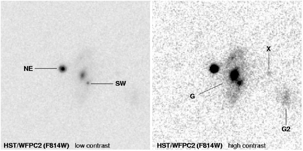
Figure 1: HST Image of J2004–1349. North is up and east is left. The quasars are separated by $1\farcs 13$.

Figure 1 shows the final $I$-band image, at low contrast (left panel) and high contrast (right panel). The quasars are labeled NE and SW. The lens galaxy, G, is a spiral galaxy. It has a prominent bulge and a disk extending nearly north–south. Two loosely wound spiral arms are visible, spiralling clockwise as they emerge from the eastern and western sides of the bulge and extend north and south. The spiral arms are more obvious in the image shown in Figure 3, in which the quasars and an elliptically symmetric galaxy model have been subtracted using a procedure described below. The SW quasar passes through the southern spiral arm, close to the bulge. The $I$-band images also revealed a faint neighboring galaxy, G2, and another object, X. Object X seems extended but it is too faint to rule out the possibility that it is a foreground star. In $V$-band, the quasars and the lens galaxy bulge were detected, but with a lower signal-to-noise ratio. From the HST images we obtained the following information:

Relative positions. We measured the relative positions of the quasars and lens galaxy with point-spread-function (PSF) fitting, using a nearby star as an empirical PSF (star #3 from the finding chart of Winn et al. 2001). We modeled the quasars as point sources, and the galaxy bulge as an elliptical exponential profile convolved with the PSF. Errors were estimated by the variance in results of fits to three sub-images, each of which was constructed from only one-third of the data. The quasar separation agreed with the more precise value determined by Winn et al. (2001) using very-long-baseline interferometry. The lens galaxy position is given in Table 1 along with other constraints used in lens models (§ 4). The result did not change significantly when the lens galaxy was modeled with an elliptical Gaussian profile or a de Vaucouleurs profile.

Flux ratio. The quasar flux ratio (NE/SW) is 8:1 in $I$-band and 20:1 in $V$-band, as compared to 1:1 at radio wavelengths. The SW quasar image is significantly redder than the NE quasar image. In § 3 we describe data that extend the measurements to near-infrared wavelengths and discuss the interpretation.

Position angle and axis ratio of the disk. By overplotting ellipses on the $I$-band image, we visually measured the position angle of the galaxy disk, $\theta_{l}=-6\fdg 5\pm 3\fdg 5$, and its projected axis ratio, $q_{l}=0.41\pm 0.05$. We use the subscript $l$ to distinguish properties of the luminosity distribution from properties of the mass distribution, which we will denote with the subscript $m$. Assuming the galaxy is intrinsically a flat circular disk, the inclination is given by $i=\cos^{-1}q_{l}=66\arcdeg\pm 3\arcdeg$.

Standard magnitudes. To measure the galaxy flux, we used a $1\farcs 5\times 2\farcs 5$ rectangular aperture centered on the bulge, after subtracting the quasars. Table 2 gives the magnitudes, using the Dolphin (2000) zero points of 21.654 for $I$ and 22.551 for $V$. The total magnitudes agree with the ground-based photometry of Winn et al. (2001), but the magnitudes of the individual components do not agree. This is because of the much poorer angular resolution of the ground-based images. In particular, what was previously identified as the SW quasar in the ground-based images is now known to be mainly light from the lens galaxy bulge.

Component	F814W $\approx I$	F555W $\approx V$
NE	$22.06\pm 0.02$	$24.54\pm 0.04$
SW	$24.56\pm 0.11$	$27.79\pm 0.41$
G	$21.62\pm 0.03$	$24.30\pm 0.16$

Table 2 — HST photometry. Error estimates represent statistical error only, and do not include the zero point error of $\approx$0.05 mag or CTE effects.

Surface brightness profile. Figure 2 shows the surface brightness of the galaxy averaged over elliptical contours. We experimented with several parametric fits to the surface brightness profile, and found the best results for a model consisting of the sum of two exponential profiles with scale lengths $0\farcs 064$ and $0\farcs 65$. The solid line shows the profile of the model after convolving with the PSF. The dashed and dotted lines show the contributions from each of the two components. The model is a good fit except for the “bump” at a semi-major axis of $0\farcs 8$ due to the spiral arms. The arms are obvious in Figure 3, which shows the residual image after subtracting the quasars and galaxy model. In this model, the bulge-to-disk flux ratio is $0.33\pm 0.07$, where the disk flux includes the total residual flux within the rectangular aperture described above.

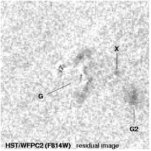
Figure 2: (left) Surface brightness of the lens galaxy, averaged over ellipses with position angle $\theta_{l}=-6\fdg 5$ and axis ratio $q_{l}=0.41$. Error bars show the variance of the points used to compute the average. The lines show the corresponding surface brightness profile of the components in the model image.

Figure 3: (right) Residual $I$-band image (= data $-$ quasar model $-$ galaxy model).

3 Differential extinction

The HST images showed that the SW quasar image is redder than the NE quasar image. This trend was confirmed with near-infrared images obtained on 2002 June 29 with the Baade 6.5m (Magellan I) telescope and Classic-Cam, a 256² HgCdTe imager with $0\farcs 115$ pixels. We obtained 52.5 minutes’ integration in $J_{s}$ and 44 in $K_{s}$, both in $0\farcs 4$ seeing and non-photometric conditions. The data were reduced in the standard fashion. We measured the quasar flux ratio using the same PSF-fitting procedure that was used for the HST images, except that in this case we locked the relative positions (and structural parameters of the galaxy) at the HST-derived values and allowed only the fluxes to vary. The uncertainty was estimated by the spread in results obtained for different choices of the lens galaxy profile. Table 3 gives the quasar flux ratio at optical and near-infrared wavelengths.

Band	Central wavelength ($\mu$m)	Flux ratio (NE/SW)
$V$	$0.555$	$20\pm 8$
$I$	$0.814$	$8.3\pm 0.7$
$J_{s}$	$1.24$	$2.7\pm 0.4$
$K_{s}$	$2.16$	$1.44\pm 0.09$

Table 3 — Quasar flux ratio.

Because gravitational lensing does not alter the wavelength of photons, the different colors of NE and SW require explanation. The most likely explanation is that SW is being reddened by dust as its light passes through the spiral arm of the lens galaxy. Differential reddening has been observed in many lens systems (Nadeau et al. 1991, Falco et al. 1999), including the spiral lens B1600+434 (Jaunsen & Hjorth 2002). The main alternative explanations are microlensing and intrinsic variability. Microlensing causes color changes if the angular size of the quasar is unresolved (which is always the case at optical wavelengths) and varies with wavelength, because microlensing magnification depends on source size (Wambsganss & Paczynski 1991; see Wucknitz et al. 2003 for a recent example). Intrinsic variability can also cause color changes when the time delay is longer than the time scale of variations and the degree of variability depends on wavelength. But neither of these alternative hypotheses is expected to produce color differences as large as observed here, and neither one would naturally explain why SW is systematically redder than NE.

To verify that the dust explanation is reasonable, we compare the wavelength-dependence of the quasar flux ratio, $f_{\lambda}({\rm NE})/f_{\lambda}({\rm SW})$, with what would be expected from dust reddening. For simplicity we assume that NE is unaffected by dust, and that intrinsic variability is negligible. Because the radio flux density ratio is 1:1, any differences in the observed magnitudes $m_{\lambda}$ should be due to extinction $A_{\lambda}$:

$$m_{\lambda}({\rm SW})-m_{\lambda}({\rm NE})=-2.5\log_{10}\frac{f_{\lambda}({\rm SW})}{f_{\lambda}({\rm NE})}=A_{\lambda}({\rm SW}).$$ (1)

We compare the observations with an extinction law $A_{\lambda}/A_{V}$ determined by Cardelli, Clayton, & Mathis (1989), using the standard Galactic value $R_{V}=3.1$, and adjusting the wavelength scale as appropriate for the lens redshift. There are 2 adjustable parameters, $E(B-V)$ and $z_{\rm lens}$, and 4 flux ratio measurements. The best fit ($\chi^{2}=1.4$) is achieved for $E(B-V)=0.97$ and $z_{\rm lens}=0.16$, which are both reasonable values. The measurements and the fitted extinction curve are shown in Figure 4. We conclude that differential extinction is a good explanation for the color difference, although it is certainly possible that microlensing and intrinsic variability also contribute to the color difference.

Following Jean & Surdej (1998), this can be regarded as a measurement of the lens redshift, but it is a crude one: the range of lens redshifts giving $\Delta\chi^{2}<1$ is $0.03<z_{\rm lens}<0.36$. In addition, the result depends on the choice of $R_{V}=3.1$. Larger values of $R_{V}$ favor smaller lens redshifts and smaller values of $R_{V}$ allow for large lens redshifts. As an example, a solution with $R_{V}=2.1$ and $z_{\rm lens}=0.9$ is also plotted in Figure 4.

Measured extinction of quasar image SW (see Eq. 1) compared to two model extinction laws from Cardelli, Clayton, & Mathis (1989).

4 Lens models

4.1 Power-law models

We consider lens models constrained by the image positions and magnification ratio (as approximated by the radio flux density ratio) given in Table 1. The uncertainties in the quasar positions and magnification ratio were enlarged from the observational uncertainties to 1 milliarcsecond and 10%, respectively, to account for systematic effects due to mass substructure (see, e.g., Mao & Schneider 1998, Metcalf & Zhao 2002, Dalal & Kochanek 2002). With only these constraints, we are restricted to simple lens models. Circular models are too simple because the lens center does not lie along the line joining the quasars. We therefore ask: what is the required ellipticity and position angle of the mass distribution? From the qualitative theory presented by Saha & Williams (2003), we expect the answer to be fairly model-independent.

We used the “power-law” family of mass models,

$$\kappa(\xi)=\frac{1}{2}\left(\frac{b}{\xi}\right)^{2-\alpha},$$ (2)

where $\kappa$ is the projected surface density (in units of $\Sigma_{\rm crit}$, the critical density for strong lensing), $\xi$ is the elliptical coordinate in the image plane, and $b$ is the Einstein radius. Implicit in $\xi$ are 4 parameters: the coordinates of the lens center, the projected axis ratio $q_{m}$, and the position angle $\theta_{m}$. The exponent $\alpha$ determines the rotation curve: $v(r)\propto r^{\alpha-1}$. The rotation curve is flat for $\alpha=1$, the isothermal case, and the physically plausible range is $0<\alpha<2$. With two additional parameters for the source coordinates, the number of parameters exceeds the number of constraints by one, leading to a one-dimensional family of models that fit the data exactly. We used software written by Keeton (2001) to optimize the model parameters for a given choice of $q_{m}$ and $\theta_{m}$, by minimizing $\chi^{2}$ in the source plane (Kayser et al. 1989, as modified by Kochanek 1991).

Figure 5 shows the contours of $\chi^{2}$ in the $(q_{m},\theta_{m})$ plane. The line of best-fit solutions is nearly horizontal. The direction of the mass quadrupole is therefore well-constrained by the image configuration even though the radial density profile is not constrained. As one moves from left to right along this line, the mass distribution becomes shallower, with $\alpha$ increasing from $0\rightarrow 2$. Along the $\chi^{2}=0$ curve, points are plotted at intervals of $\Delta\alpha=0.1$ with a symbol size proportional to $\alpha$. The value of $\alpha$ is indicated explicitly for four representative models. The caustics and critical curves of those four models are shown in Figure 6. Over almost the entire range of $\alpha$, the position angle of the mass model agrees with the position angle of the luminous galaxy disk.

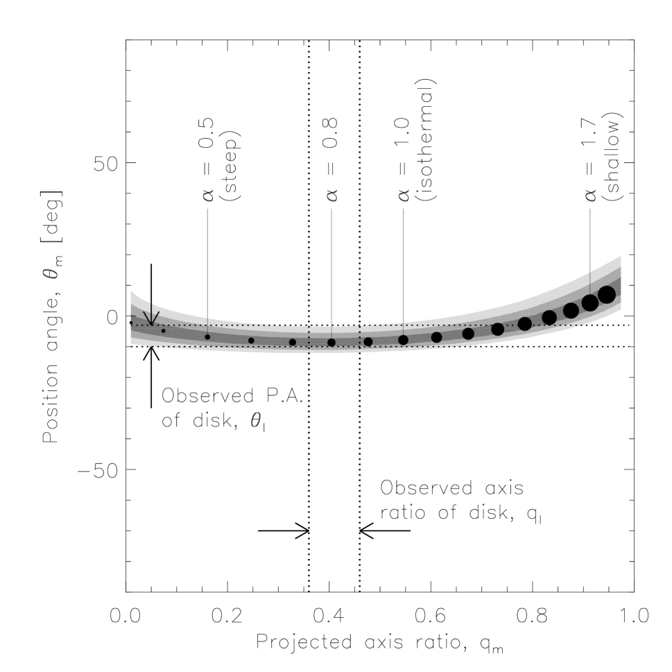
Figure 4: Allowed power-law models of J2004–1349. Gray levels represent $\chi^{2}<1$, 4, and 9. Along the $\chi^{2}=0$ curve, points are plotted at intervals of $\Delta\alpha=0.1$ with a symbol size proportional to $\alpha$. Dotted lines indicate the values determined from the HST $I$-band image.

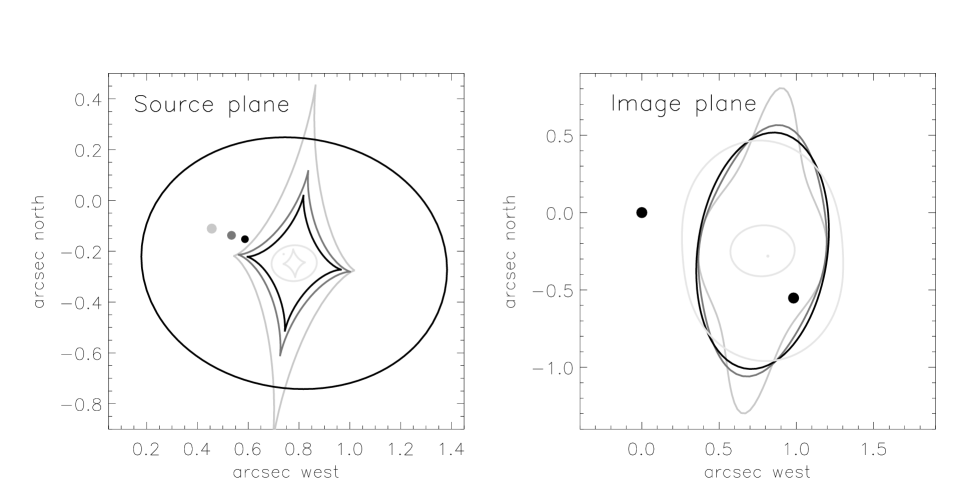
Figure 5: Lens models of J2004–1349 for $\alpha=1$ (black), $\alpha=0.8$ (dark gray), $\alpha=0.5$ (light gray), and $\alpha=1.7$ (lightest gray). The left panel shows the caustics and source positions. The right panel shows the critical curves and image positions. The innermost ellipse and dot are the radial critical curve and third image of the $\alpha=1.7$ model. Source and image fluxes are proportional to the area of the dots.

The models for which the mass and light are not quite co-aligned seem less plausible, on other grounds, than the co-aligned models. They are very shallow ($\alpha>1.49$), corresponding to a rapidly rising rotation curve at a radius comparable to the disk scale length. They have a large radial critical curve (which does not exist for $\alpha\leq 1$) and, within this curve, a third quasar image. These models are illustrated by the $\alpha=1.7$ case in Figure 6. In that case, the predicted third image has 7% of the flux of each bright image. Current radio maps limit the flux of a third image to $<$2% of the flux of each quasar image (Winn et al. 2001). The shallow models also have small caustics (and consequently small lensing cross-sections), large Einstein radii, and large magnifications ($b=3\farcs 6$ and $\mu_{\rm total}=50$, for $\alpha=1.7$).

Therefore, for the most plausible range of mass distributions, the mass and light are co-aligned. Another way to state the result is that we can put only a very weak one-sided limit on the rotation curve ($\alpha<1.49$) by requiring the mass quadrupole to be aligned with the luminous disk ($\theta_{l}=\theta_{m}$). If we require that the light and mass agree both in position angle and projected axis ratio ($\theta_{l}=\theta_{m}$ and $q_{l}=q_{m}$), the result is $\alpha=0.80\pm 0.08$. However, the latter requirement is too simplistic because it ignores the contribution of the dark halo, which one might expect to be rounder than the disk.

Consider, for example, the case of a flat rotation curve: $\alpha=1$. Figure 6 shows that such a model must be rounder than the observed disk ($q_{m}=0.55>0.41=q_{l}$). As pointed out by Keeton & Kochanek (1998), the $\alpha=1$ model can be interpreted as the projection of either an intrinsically flat Mestel disk, or a singular isothermal ellipsoid (SIE). The disagreement of $q_{m}$ and $q_{l}$ rules out a pure Mestel disk, but a SIE halo is allowed. In terms of the three-dimensional axis ratio $q_{3m}$, the projected axis ratio $q_{m}$ of an oblate ellipsoid is

$$q_{m}^{2}=\sqrt{q_{3m}^{2}\sin^{2}i+\cos^{2}i},$$ (3)

giving $q_{3m}=0.38\pm 0.08$ in this case. Thus, assuming a flat rotation curve, a pure-halo model must be very oblate.

4.2 Models with bulge, disk, and halo

Next, we consider models with separate mass components for the bulge, disk, and halo. Based on the HST surface photometry of § 2, we described the bulge and disk by exponential functions,

$$\kappa(\xi)=\kappa_{0}\exp(-\xi/R_{i}),$$ (4)

fixing the scale lengths of the bulge and disk to be $R_{b}=0\farcs 064$ and $R_{d}=0\farcs 65$. We required the axis ratio and position angle of each component to be $0.41\pm 0.05$ and $-6\fdg 5\pm 3\fdg 5$, to agree with the HST-measured values, by adding appropriate terms to the $\chi^{2}$-function with the software by Keeton (2001). We allowed the the central surface density (or, equivalently, the total mass $M$) of each component to vary. With only these two components, there is one degree of freedom. Even without any dark-matter halo, the model provides an excellent fit to the data, with $\chi^{2}_{\rm min}=0.1$ and $M_{b}/M_{d}=0.16\pm 0.03$ for $\Delta\chi^{2}<1$.

This result and its error bar are internal to our particular bulge/disk decomposition, but the result is fairly robust, as long as the bulge is taken to be much more centrally concentrated than the disk. For $R_{b}=0\farcs 08$, the maximum value consistent with the HST image, the result changes only slightly, to $M_{b}/M_{d}=0.18$. The other extreme, taking the bulge to be a point mass, gives $M_{b}/M_{d}=0.14$. The latter case also demonstrates that the shape of the bulge is not significant; a perfectly round bulge with $R_{b}=0\farcs 064$ gives $M_{b}/M_{d}=0.15$. The disk scale length $R_{d}$ is harder to measure in the HST image, because of the low surface brightness of the disk and the patchiness of the arms, but even for $R_{d}=1\arcsec$ the bulge-to-disk mass ratio is 0.11. Hence, insofar as both components can be approximated by exponential mass distributions, the bulge-to-disk mass ratio is $0.16\pm 0.05$.

We used the single degree of freedom to investigate how this result changes with the inclusion of the dark halo. We described the dark halo as a spherical isothermal profile with a constant-density core,

$$\kappa(R)=\frac{b}{2}\frac{1}{\sqrt{R^{2}+s^{2}}},$$ (5)

adding two extra parameters: the Einstein radius $b$ and the core radius $s$. We do not consider flattened haloes, because with the present number of constraints, we would only be able to trace out the degeneracies between model parameters, which has already been done in detail by Koopmans, de Bruyn, & Jackson (1998) and Maller et al. 2000 for the case of B1600+434. Even with a spherical halo, the number of parameters exceeds the number of constraints by one, and there is a one-dimensional family of solutions with $\chi^{2}=0$. We found all the solutions with $0\arcsec\leq b\leq 2\arcsec$ and, in each case, determined the net rotation curve and bulge-to-disk mass ratio.

The spherical halo does not significantly change the derived bulge-to-disk mass ratio. The full range of values of $M_{b}/M_{d}$ is 0.13–0.17. The explanation is that when $b$ is large enough to contribute significantly to the deflection, the optimized core radius is also large, giving the halo a nearly constant density in the vicinity of the quasar images. This nearly constant-density sheet affects only the optimized position and flux of the source. The relative image positions and fluxes are controlled by the mass components representing the bulge and disk.

Rotation curve of the bulge+disk+halo model described in § 4.2.

Although the rotation curve of the lens galaxy has not been measured, most disk galaxies have fairly flat rotation curves. From all the disk+bulge+halo models, we determined the one with the flattest rotation curve (smallest mean-squared deviation from a straight line) in the range $R_{b}<r<4R_{d}$. This model has $M_{b}/M_{d}=0.16$ and the rotation curve is plotted in Figure 7. The individual rotation curves of the bulge, disk, and halo are also plotted. Because the redshifts of the lens and source are unknown, the velocity must be plotted in dimensionless units $v(R)/\sqrt{2GD_{L}\Sigma_{\rm crit}}$, where $D_{L}$ is the angular-diameter distance to the lens, and $\Sigma_{\rm crit}$ is the critical density for strong lensing.

5 Summary and discussion

We have shown that PMN J2004–1349 has a spiral lens galaxy, making it one of only a handful of spiral lenses known to date. Uniquely, the lens has an accurately-measured position, does not have a very massive neighbor, and is not collinear with the quasar images, which has allowed us to test whether the mass quadrupole is aligned with the luminous disk. The direction of the quadrupole is well constrained even though the radial density distribution is poorly constrained. We found that the mass and light are aligned within a few degrees, except for very shallow mass distributions that appear physically implausible. This had been shown previously for elliptical galaxies, especially by Keeton, Kochanek, & Seljak (1997), Keeton, Kochanek, & Falco (1998), and Kochanek (2002), with increasingly large samples. However, this had not been shown before for spiral galaxies, owing to problems with those few examples of spiral lenses currently known.

This conclusion would be weakened if tidal gravitational forces (“external shear”) from neighboring masses are producing some of the observed non-collinearity. One might regard the close alignment of the light and mass as an argument against a large shear. The only neighbors visible in the HST images, G2 and X, are faint (with fluxes $\sim$10% and $\sim$1% that of G) and are not positioned along the disk axis where they would produce the maximum effect.

Using the axis ratio, position angle, and scale lengths measured in the HST image, we tested a model consisting of a bulge and disk with constant mass-to-light ratios. The model successfully reproduces the image configuration for a bulge-to-disk mass ratio of $0.16\pm 0.05$, a conclusion that does not change if a spherical dark-matter halo is added to produce a flat rotation curve. In $I$-band, the bulge-to-disk flux ratio was found to be $0.33\pm 0.07$, implying $(M/L)_{b}/(M/L)_{d}=0.5\pm 0.2$ in $I$-band. This is a counter-intuitive result, because one expects disks to contain more young and massive stars (with smaller mass-to-light ratios) than bulges. A flattened halo would reduce the disk mass, but current data do not provide enough constraints to do more than trace out this degeneracy. It would be interesting to assess the stellar populations of the bulge and disk, and the possible effect of internal extinction in the disk, using multi-color HST images. The current $V$-band images are too shallow to provide useful color information for the bulge and disk separately.

A high priority for future work is spectroscopy of the lens galaxy and source quasar. Knowledge of the redshifts of lens and source are essential for computing and interpreting the mass-to-light ratios of the lens galaxy. Measurement of the circular velocity of the lens galaxy would break modeling degeneracies between different mass distributions with the same projected surface density (for analogous work on elliptical galaxies, see e.g. Falco et al. 1997, Tonry 1998, Romanowsky & Kochanek 1999, Koopmans & Treu 2002).

It may also be possible to measure the time delay between flux variations of the quasar images, which depends sensitively on the radial mass profile. Or, conversely, it may be possible to measure the Hubble constant using the Refsdal (1964) method, if the radial density profile is determined by other means. Sensitive radio observations may detect a third quasar image, or lensed radio jets emerging from the quasar cores, which can discriminate between different radial mass profiles (Rusin et al. 2002; Winn, Rusin, & Kochanek 2003). Finally, if the sample of spiral lenses can be greatly expanded, it may be possible to use the ensemble of lens data to place statistical constraints on spiral galaxy structure, as has been done for elliptical galaxies (Rusin, Kochanek, & Keeton 2003). The enticing potential of gravitational lensing to probe the mass distribution of spiral galaxies will depend on the success of at least some of these proposed observations.

References

- Bartelmann & Loeb (1998) Bartelmann, M. & Loeb, A. 1998, ApJ, 503, 48
- Cardelli, Clayton, & Mathis (1989) Cardelli, J. A., Clayton, G. C., & Mathis, J. S. 1989, ApJ, 345, 245
- Combes (2002) Combes, F. 2002, New Astronomy Reviews, 46, 755
- Corteau & Rix (1999) Corteau, S. & Rix, H.-W. 1999, ApJ, 513, 561
- Courbin et al. (2002) Courbin, F., Meylan, G., Kneib, J.-P., & Lidman, C. 2002, ApJ, 575, 95
- Dalal & Kochanek (2002) Dalal, N. & Kochanek, C. S. 2002, ApJ, 572, 25
- Dolphin (2000) Dolphin, A.E. 2000, PASP, 112, 1397
- Falco et al. (1997) Falco, E. E., Shapiro, I. I., Moustakas, L. A., & Davis, M. 1997, ApJ, 484, 70
- Falco et al. (1999) Falco, E. E. et al. 1999, ApJ, 523, 617
- Fruchter & Hook (2001) Fruchter, A.S. & Hook, R.N. 2001, PASP, 114, 144
- Huchra et al. (1985) Huchra, J., Gorenstein, M., Kent, S., Shapiro, I., Smith, G., Horine, E., & Perley, R. 1985, AJ, 90, 691
- Jackson et al. (1995) Jackson, N. et al. 1995, MNRAS, 274, L25
- Jaunsen & Hjorth (1997) Jaunsen, A. O. & Hjorth, J. 1997, A&A, 317, L39
- Jean & Surdej (1998) Jean, C. & Surdej, J. 1998, A&A, 339, 729
- Kayser et al. (1990) Kayser, R., Surdej, J., Condon, J. J., Kellermann, K. I., Magain, P., Remy, M., & Smette, A. 1990, ApJ, 364, 15
- Keeton (2001) Keeton, C.R. 2001, preprint [astro-ph/0102340]
- Keeton (2003) Keeton, C. R. 2003, ApJ, 582, 17
- Keeton, Kochanek, & Seljak (1997) Keeton, C. R., Kochanek, C. S., & Seljak, U. 1997, ApJ, 482, 604
- Keeton, Kochanek, & Falco (1998) Keeton, C.R., Kochanek, C.S., & Falco, E.E. 1998, ApJ, 509, 561
- Kochanek (1991) Kochanek, C. S. 1991, ApJ, 373, 354
- Kochanek (2002) Kochanek, C. S. 2002, in “The Shapes of Galaxies and Their Dark Matter Halos”, Proc. Yale Cosmology Workshop, ed. P. Natarajan, World Scientific (Singapore) p. 62
- Koopmans, de Bruyn, & Jackson (1998) Koopmans, L.V.E., de Bruyn, A.G., & Jackson, N. 1998, MNRAS, 295, 534
- Koopmans & Treu (2002) Koopmans, L. V. E. & Treu, T. 2002, ApJ, 568, L5
- Lehár et al. (2000) Lehár, J., Falco, E.E., Kochanek, C.S., McLeod, B.A., Muñoz, J.A., Impey, C.D., Rix, H.-W., Keeton, C.R., & Peng, C.Y. 2000, ApJ, 536, 584
- Maller, Flores, & Primack (1997) Maller, A.J., Flores, R.A., & Primack, J.R. 1997, ApJ, 486, 681
- Maller et al. (2000) Maller, A.H., Simard, L., Guhathakurta, P., Hjorth, J., Jaunsen, A.O., Flores, R.A., & Primack, J.R. 2000, ApJ, 533, 194
- Mao & Schneider (1998) Mao, S. & Schneider, P. 1998, MNRAS, 295, 587
- Mao, Witt, & Koopmans (2001) Mao, S., Witt, H. J., & Koopmans, L. V. E. 2001, MNRAS, 323, 301
- Metcalf & Zhao (2002) Metcalf, R. B. & Zhao, H. 2002, ApJ, 567, L5
- Möller & Blain (1998) Möller, O. & Blain, A.W. 1998, New Astronomy Reviews, 42, 93
- Palunas & Williams (2000) Palunas, P. & Williams, T.B. 2000, AJ, 120, 2884
- Patnaik et al. (1993) Patnaik, A. R., Browne, I. W. A., King, L. J., Muxlow, T. W. B., Walsh, D., & Wilkinson, P. N. 1993, MNRAS, 261, 435
- Perna, Loeb, & Bartelmann (1997) Perna, R., Loeb, A., & Bartelmann, M. 1997, ApJ, 488, 550
- Pramesh Rao & Subrahmanyan (1988) Pramesh Rao, A. & Subrahmanyan, R. 1988, MNRAS, 231, 229
- Refsdal (1964) Refsdal, S. 1964, MNRAS, 128, 307
- Romanowsky & Kochanek (1999) Romanowsky, A. J. & Kochanek, C. S. 1999, ApJ, 516, 18
- Rusin et al. (2002) Rusin, D., Norbury, M., Biggs, A. D., Marlow, D. R., Jackson, N. J., Browne, I. W. A., Wilkinson, P. N., & Myers, S. T. 2002, MNRAS, 330, 205
- Rusin, Kochanek, & Keeton (2003) Rusin, D., Kochanek, C.S., & Keeton, C.R. 2003, ApJ, in press [astro-ph/0306096]
- Sackett (1997) Sackett, P.D. 1997, ApJ, 483, 103
- Sackett (1999) Sackett, P.D. 1999, in Galaxy Dynamics, eds. D.R. Merritt, M. Valluri, & J.A. Sellwood, ASP Conference Series vol. 182 (San Francisco: ASP), p. 393
- Saha & Williams (2003) Saha, P. & Williams, L. L. R. 2003, AJ, 125, 2769
- Schmidt, Webster, & Lewis (1998) Schmidt, R., Webster, R. L., & Lewis, G. F. 1998, MNRAS, 295, 488
- Sofue & Rubin (2001) Sofue, Y. & Rubin, V. 2001, ARA&A, 39, 137
- Tonry (1998) Tonry, J. L. 1998, AJ, 115, 1
- Trott & Webster (2002) Trott, C. M. & Webster, R. L. 2002, MNRAS, 334, 621
- van Albada & Sancisi (1986) van Albada, G.D. & Sancisi, R. 1986, Phil. Trans. R. Soc. London A, 320, 447
- Wambsganss & Paczynski (1991) Wambsganss, J. & Paczynski, B. 1991, AJ, 102, 864
- Wang & Turner (1997) Wang, Y. & Turner, E. L. 1997, MNRAS, 292, 863
- Winn et al. (2001) Winn, J.N., Hewitt, J.N., Patnaik, A.R., Schechter, P.L., Schommer, R.A., López, S., Maza, J., & Wachter, S. 2001, AJ, 121, 1223
- Winn et al. (2002) Winn, J.N., Kochanek, C.S., McLeod, B.A., Falco, E.E., Impey, C.D., & Rix, H.-W. 2002, ApJ, 575, 103
- Winn, Rusin, & Kochanek (2003) Winn, J. N., Rusin, D., & Kochanek, C. S. 2003, ApJ, 587, 80
- Wucknitz et al. (2003) Wucknitz, O., Wisotzki, L., Lopez, S., & Gregg, M.D. 2003, preprint [astro-ph/0304435]