A Chandra Observation of the Diffuse Emission in the Face-on Spiral NGC 6946

Abstract

This paper describes the Chandra observation of the diffuse emission in the face-on spiral NGC 6946. Overlaid on optical and H${\alpha}$ images, the diffuse emission follows the spiral structure of the galaxy. An overlay on a 6 cm polarized radio intensity map confirms the phase offset of the polarized emission. We then extract and fit the spectrum of the unresolved emission with several spectral models. All model fits show a consistent continuum thermal temperature with a mean value of 0.25$\pm$0.03 keV. Additional degrees of freedom are required to obtain a good fit and any of several models satisfy that need; one model uses a second continuum component with a temperature of 0.70$\pm$0.10 keV. An abundance measure of 3${}^{+1.95}_{-1.90}$ for Si differs from the solar value at the 90% confidence level; the net diffuse spectrum shows the line lies above the instrumental Si feature. For Fe, the abundance measure of 0.67$\pm$0.13 is significant at 99%. Multiple gaussians also provide a good fit. Two of the fitted gaussians capture the O VII and O VIII emission; the fitted emission is consistent with an XMM-Newton RGS spectrum of diffuse gas in M81. The ratio of the two lines is $<$0.6-0.7 and suggests the possibility of non-equilibrium ionization conditions exist in the ISM of NGC 6946. An extrapolation of the point source luminosity distribution shows the diffuse component is not the sum of unresolved point sources; their contribution is at most 25%.

1 Introduction

The total X-ray emission from a spiral galaxy consists of the sum of the emission from its X-ray-emitting constituents including X-ray binaries (low-mass and high-mass), supernova remnants, OB star clusters, other point sources, and the hot component of the interstellar medium. This last component is expected to be present based upon the theoretical work of McKee & Ostriker (1977) and Norman & Ikeuchi (1989) among many others. Prior to the launch of Chandra and XMM-Newton, the hot component had been detected in a handful of galaxies, largely as a consequence of the broad spatial resolution of previous X-ray telescopes which distributed X-rays from point sources over a wide region of the galaxy, contaminating any signal from the hot ISM.

The study of the X-ray emission from normal galaxies commenced with the Einstein observations of galaxies (for a review, see Fabbiano 1989). The spatial resolution of Einstein, $\sim$1^′ (e.g., Hartline 1979), prevented separation of the X-ray emitting constituents for all but the nearest galaxies. ROSAT improved the resolution by about three times, providing views of a broader range galaxies outside the Local Group (e.g., Roberts & Warwick 2001). The use of Chandra and XMM-Newton has led to more detections because of the large effective area of XMM-Newton and the sharp point spread function of Chandra.

NGC 6946 is a well-studied face-on spiral initially detected in X-rays with the Einstein Observatory (Fabbiano & Trinchieri, 1987). Schlegel (1994) obtained a 36-ksec pointing using the ROSAT PSPC, detected 9 point sources, and reported the existence of a diffuse component with a temperature of 0.55 keV (90% error range of 0.3-0.65 keV) which we will show just overlaps with the results to be presented. That study argued that the diffuse component was truly diffuse and not the summed emission of point sources based upon a plausibility argument for the expected numbers of sources of various types. In a separate study, Schlegel, Blair, & Fesen (2000) described a ROSAT HRI observation as well as an observation using ASCA. In this case, the high internal background of the HRI prevented a detection of the diffuse component, while the broad PSF of the ASCA mirrors blended events from the known point sources with the diffuse emission.

This paper describes the diffuse emission in NGC 6946 revealed by a 60-ksec Chandra observation of the galaxy. The point source population has been described by Holt et al. (2003). The primary goal of this paper is a spectrum of the diffuse emission. Following this introduction, we describe our analysis steps, then present a brief comparison of the diffuse emission with images from other bandpasses, followed by a longer analysis of the spectral fits and a discussion of the results.

Chandra presents a unique opportunity to observe the diffuse component as free as may be possible, at least for the foreseeable future, from contamination by point sources. The Chandra mirrors deliver $\sim$80% of the X-rays at 1 keV into a circle $\sim$0.7 arcsec in radius and 70% into a 0.7 arcsec radius circle at 6 keV. At 5^′ off-axis, the corresponding numbers are 90% into a circle of a radius $\sim$2^′′.5 at 1 keV and $\sim$4^′′ radius at 6 keV (CXC Proposers’ Guide, 2002).

The adopted distance for NGC 6946 is 5.9 Mpc (Karachentsev et al., 2000) with a corresponding scale of 1^′′ $\sim$29 pc. The column density in the direction of NGC 6946 is $\sim$3-5$\times$10²¹ cm^-2 (Schlegel, Finkbeiner, & Davis, 1998).

2 Observation Summary

Chandra observed NGC 6946 on 2001 September 7. The galaxy was imaged on the back-illuminated (BI) chip S3. The data were examined for flares to which the BI chip is susceptible, but no flares with a count rate greater than 0.04 counts s^-1 were located; screening any flare-like spikes removed 1296 sec of the 59116 sec observation, leaving a net on-source, deadtime-corrected, exposure of 57819 sec.

The data were filtered to eliminate events with energies below 0.3 keV and above 8 keV. The low-energy cut does not remove source photons because those events are lost to the high column in the direction of the galaxy. The high cut removes extraneous cosmic ray-generated events.

While the internal background of the ACIS detector is low (for S3, $\sim$0.3 counts s^-1 chip^-1, CXC Proposers’ Guide (2002)) and often may be ignored for counts from point sources extracted with a typical detection cell a few arc sec in size, the large extent of the galaxy and the faintness of the diffuse emission require a careful analysis of the background. The D₂₅ circle is $\sim$14 arcmin in size (Tully, 1988) and is larger than the ACIS S3 CCD. The large extent of the galaxy prevents the use of portions of the S3 chip outside of the galaxy as a measure of the background. We instead obtained the background from a “blank field” observation. The data were filtered identically by energy, then re-projected onto the sky using the aspect solution of the actual NGC 6946 observation. The exposure time of the background observation was $\sim$300 ksec.

Point sources were detected as described in Holt et al. (2003), using a wavelet detection that is directly tied to the point spread function’s behavior with off-axis angle (Freeman et al., 2002). The point source detection reached a limiting luminosity L_X $\sim$3$\times$10³⁶ erg s^-1 in the 0.3-5 keV band which corresponded to $\sim$10 counts. Holt et al. (2003) deemed the source detection complete to $\sim$1$\times$10³⁷ erg s^-1; the completeness limit is lower by $\sim$30% near the center of the CCD because of the sharper point spread function there where $\sim$7-8 counts constitutes a detection. Most of the detected diffuse emission lies within 2.5-3 arcmin of the aimpoint. We do not see a trend of increasing numbers of weak sources as we approach the aimpoint, suggesting a relative lack of contamination of the diffuse emission by weak point sources. We postpone until §5 a longer discussion of the impact of possible unresolved point sources.

Sources were removed from the data using the CIAO tool dmfilth which cuts out each source, then replaces the resulting ‘hole’ by sampling the events in annuli surrounding the locations of the sources. The extraction apertures used enclosed $>$95% of the encircled energy. The annuli had inner radii 25% larger than the radii of the source extraction circles. Care was taken to ensure that the annular sampling did not include any source events. Figure 1 shows the results of all the steps just described: the energy-filtered data, minus point sources, and binned into 4-arcsec pixels. Immediately from the raw data (Figure 1) we see the diffuse emission as well as bright areas, particularly on the N and W arms and surrounding the nucleus.

We then adaptively smoothed the data using the CIAO code csmooth. We adopted a gaussian smoothing kernel and selected the smoothing parameter to be 3${\sigma}$ as calculated locally. Finally, we subtracted a constant from the result to remove the overall background as determined by the ‘blank field’ background. Figure 2 shows the results in the three bands. The 0.3-0.6 keV band shows little emission specific to NGC 6946 because of the high column in the galaxy’s direction. The 0.6-0.9 and 0.9-2 keV bands appear similar: contours fall in similar regions of the galaxy in each band. In the 0.9-2 keV image, the apparent emission that extends beyond the region defined by the 0.6-0.9 keV image is an artifact of the adaptive smoothing, driven by the lower counts in the 0.9-2 keV band. We henceforth use just the 0.6-0.9 keV band for any comparisons. The “point sources” apparent in this figure do not correspond with any of the detected sources listed in Holt et al. (2003), nor do they correspond with point sources lying below the threshold. An examination of the raw data at full resolution shows a broad distribution of counts suggestive of a diffuse but clumpy source.

3 Multiwavelength Comparison

In this section we compare the X-ray image of the diffuse emission with images obtained in other bandpasses.

The apparent “point sources” discussed at the end of the previous section do not correspond to any of the optically-identified supernova remnants (Matonick & Fesen, 1997). The regions may correspond with prominent H II regions identified in the submillimeter band by Alton et al. (2002). The extracted counts from these regions yield luminosities of $\sim$1.5$\times$10³⁷ erg s^-1 using a simple thermal bremsstrahlung model with temperature of 0.3 keV (§4.4).

Figure 3 shows the contours of the 0.6-0.9 keV emission overlaid on an H${\alpha}$ image. Note that in general the X-rays follow the H${\alpha}$ emission. This behavior is most easily visible on the prominent northern arm or at the sharp south-southeast edge. The weak arm to the northwest is not detected; nor is the weaker portion of the inner eastern arm. The matching behavior means that the X-ray emission arises from a hot diffuse ISM component or from the summed emission of point sources confined to the arms. We will return to this question in the discussion section.

Figure 4 shows the 0.6-0.9 keV X-ray contours over the 6-cm polarized intensity map from (Beck & Hoernes, 1996) and discussed in Frick et al. (2001). Beck & Hoernes (1996) showed that the regular magnetic field is strongest in the interarm region. In the previous figure, we established that the X-ray emission follows the northern arm. As in Beck & Hoernes (1996), it is clear the polarized emission lies external to that arm, so the X-ray image is consistent with their result.

Figure 5 shows the 0.6-0.9 keV X-ray contours overlaid on the 850 ${\mu}$m map of Alton et al. (2002). At 850 ${\mu}$m, the nucleus as well as 3 knots of emission are prominent; the knots lie to the northeast, east, and south-southeast of the nucleus. Overall, the regions of strongest X-ray emission correspond with the regions brightest at 850 ${\mu}$m. These knots correspond to prominent H II regions. The 850 ${\mu}$m emission largely arises from dust heated by starlight and thermally radiating (e.g., Israel et al. 1999).

Figure 6 displays the 0.6-0.9 keV X-ray contours on the 3 cm thermal radio emission (available in Frick et al. 2001). In general, knots of X-ray emission align with the radio knots, particularly on the NE arm. A longer X-ray exposure is required to ascertain whether the outer regions in the 3 cm image have a corresponding X-ray counterpart.

4 Spectral Fit: Introduction

For all of the analysis, we fit the spectra of the diffuse emission $+$ background and the background simultaneously. This introduction describes the extraction of the spectra and a fit to the background.

Two approaches are generally used to extract a spectrum spread across a large expanse of the ACIS chips: (i) extract the data as small arrays, build a response matrix specific to each array, and sum the arrays; or (ii) correct the entire chip for the charge transfer inefficiencies (CTI), extract a single source$+$background spectrum, and construct one response matrix (the Penn State approach, using the CTI corrector as described in Townsley et al. 2002). We adopted the second method. A correction for the time-dependent contamination was included by reducing the effective area at each affected energy.

Following the removal of the point sources, the spectrum of the diffuse emission$+$background was extracted including all pixels within the S3 chip and with exposure $>$0.9 of the on-axis time (this eliminates edge effects). A total of 28248 counts were extracted representing the spectrum of the source plus background. A background spectrum was extracted from the reprojected blank field observation using the same (x, y) image pixels as for NGC 6946 itself. The background spectrum contained 331600 counts and 22334 counts after scaling the exposure time to that of NGC 6946. The source spectrum was adaptively binned so that the resulting spectrum contained at least 20 counts per channel.

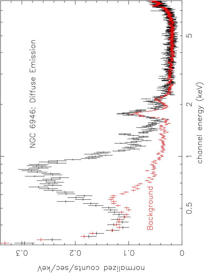
Figure 7: Plot of the diffuse + background (upper curve) and background (lower) spectra. The background spectrum was extracted from a blank sky observation after reprojecting those events using the aspect solution from the NGC 6946 observation and scaling by the ratio of the exposure times between the background and the NGC 6946 observations. The diffuse $+$ background spectrum contains 28248 counts; the background spectrum contains 22334 counts. The difference is the net spectrum of the diffuse emission and contains 5914 counts.

Figure 7 shows the two extracted spectra as an overlay. From this figure, it is clear that the galaxy’s diffuse emission fades into the background near 2 keV and is blocked below $\sim$0.5 keV by the column toward NGC 6946. This figure reinforces one’s visual impression as well as quantitative expectation: most of the visually apparent emission appears in the 1-2 keV band where Chandra’s effective area takes on the largest values. The visible ‘emission lines’ arise from particle background stimulation of material in the detectors; the large line at 1.8 keV is Si K${\alpha}$ (CXC Proposers’ Guide, 2002). The difference between the two spectra of Figure 7 represents the net diffuse spectrum and contains 5914 counts.

Figure 8 shows a fit to the background using a number of power law and gaussian components. The residuals are flat to within $\sim$15% across the bandpass. We use this background model in all subsequent spectral fitting, freezing the parameters at their best-fit values. We justify this approach by noting the background spectrum may be fitted to very high precision, it having been accumulated from numerous long exposures.

4.1 Fit to All Diffuse Emission

Simple continuum models did not provide a good fit and in all cases left clear residuals. For example, the use of a single Mekal model produced the lowest ${\chi}^{2}/{\nu}$ of 1.21 of all the single-component models, but left clear residuals in the 0.9 keV band. The residuals essentially force consideration of additional degrees of freedom.

Four models provided essentially comparable goodness-of-fit values. At the interpretation stage, we will use the results from one or more models because any one of them could be deemed ”correct.” First, we adopted a double ‘Mekal’ spectral model representing thermal emission from a diffuse gas as calculated by Mewe, Gronenschild, & van den Oord (1985); Mewe, Lemen, & van den Oord (1986) and Kaastra (1992) with Fe L calculations supplied by Liedahl, Osterheld, & Goldstein (1995). Second (and third), we used single and dual variable abundance Mekal models, allowing the abundances of species with lines in the 0.5-2 keV band to vary. Last, we fit the spectrum with a simple thermal bremsstrahlung to define the continuum and included as many gaussian lines as required by the data. For the multi-gaussian approach, the choice of continuum model is largely irrelevant, as any simple model will produce a fit. A power law, for example, works as well as a bremsstrahlung model (the resulting index is a steep $\sim$7$\pm$0.55, 90% error); we adopt the bremsstrahlung model to provide a check on the fitted temperatures from the more complex models. For the gaussian lines, we set their widths to zero, because the lines are unresolved with ACIS but broadened by the instrumental response, and their centers to the positions of expected lines (§4.3). The multi-gaussian approach provides information on the ionization states contributing to the total emission. Figure 9 (top) shows the dual variable Mekal fit while the bottom figure shows the multi-gauss fit.

We also included a power law component to account for any excess emission between the source plus background and background spectra. The residual flux from this power law ‘background’ component is $\lesssim$6% of the total diffuse flux, verifying the quality of the background definition and its separation from the diffuse emission of NGC 6946. Table 1 lists the parameters for the fitted models.

4.2 Continuum Emission

The continuum temperatures of the single continuum models or the low temperature component of the dual models are identical within the errors with kT $\sim$0.25-0.32 keV. Figure 10 (top) shows the variable Mekal model contours for the low-temperature component. The fitted column density is also identical within the errors for all models with a range of 3.6-4.1$\times$10²¹ cm^-2. These columns lie about a factor of 2 above the Dickey & Lockman column ($\sim$2$\times$10²¹ cm^-2, Dickey & Lockman 1990) but within the errors of the Schlegel, Finkbeiner, & Davis (1998) value of $\sim$3-5$\times$10²¹ cm^-2.

The integrated flux in the 0.5-2 keV band is $\sim$3.7$\times$10^-13 ergs s^-1 cm^-2 (absorbed) or $\sim$2.5$\times$10^-12 (unabsorbed). The integrated luminosity values are $\sim$1.5$\times$10³⁹ and $\sim$1$\times$10⁴⁰ erg s^-1, respectively, or $\sim$2.9$\times$10³⁷ and $\sim$1.9$\times$10³⁸ erg s^-1 arcmin^-2, respectively.

These values differ somewhat from previous measurements. The ROSAT measure of the column was low by about a factor of 2 (Schlegel, 1994). The fitted temperature is also lower than the ROSAT PSPC value of 0.55${}^{+0.10}_{-0.25}$ keV; even though the error bars just overlap, the higher temperature behavior of the ROSAT fit is not unexpected. The fitted temperature, for example, from the PSPC data was almost certainly artificially high because it included photons from sources with harder spectra, such as X-ray binaries, that were incompletely removed. In addition, §4.1 shows that two spectral components are required for a good fit with one at kT $\sim$0.7 while the PSPC data were consistent with a single temperature because of the detector’s lower spectral resolution. The integrated flux is higher than the ROSAT value by $\sim$25%, as is expected given the higher value for the column density. As an aside, the very broad PSF of the ASCA mirrors prohibited an analysis of the diffuse emission from the NGC 6946 observation (Schlegel, Blair, & Fesen, 2000).

4.3 Line Emission and Abundances

The abundances of the single variable Mekal model were first varied individually to test the size of the resulting error. An abundance, for which the 1 ${\sigma}$ error was consistent with 1.0, was reset to and fixed at 1.0. Two abundances (Si, Fe) were found to differ significantly from 1 (Figure 11). For Fe, the abundance is 0.67$\pm$0.13 solar at the 99% level. For Si, the abundance is 3.0 with the 90% contour just above 1.0 at 1.05; at 99%, the Si abundance is consistent with solar. No flares occurred during the observation, so the line is unlikely instrumental in origin. We return to this point momentarily.

The gaussian centers were fixed at the energies of potentially prominent lines, corresponding to O VII 0.57 keV, O VIII 0.653 keV, Fe I (L) 0.705 keV, Fe XVII 0.826 keV, Ne IX 0.922 keV, Fe XX 0.996 keV, Ne X 1.022 keV, and Mg XI 1.34 keV. Lines at energies lower than $\sim$0.5 keV were deemed irrelevant because of the high column toward NGC 6946. Several lines were significantly detected at $>$99% (Table 1). At the energies of these lines, the ACIS spectral resolution is $\sim$110-120 eV (CXC Proposers’ Guide, 2002).

While we fixed the line centers at specific energies to test for the presence or absence of known lines, we relaxed that requirement for the Si line to test whether the feature in the source$+$background spectrum was consistent with the background feature. The background line is best fit with a gaussian at 1.775$\pm$0.002 keV (blend of Si K${\alpha}$) while the diffuse Si line has a best-fit energy of 1.860$\pm$0.027 keV (= Si XIII).

Assume for the moment the spectral fits are accurate measures of the line emission. The presence of O VII and O VIII then provides a measure of the overall ionization in the diffuse emission. O VIII 0.653 keV is the Ly$\alpha$ transition; the blended O VII 0.57 line(s) represent the 1s2p to 1s² transition. The log of the ratio is -0.2$\pm$0.7 and has a large error because of the decreasing continuum in the 0.5-0.6 keV band and because of the energy resolution of the CCD. Nevertheless, the ratio translates to limits of 9.6 $\lesssim$ log n_et $\lesssim$12.0, where n_e represents the electron density and t the cooling time (see, for example, Vedder et al. 1986). If the low ‘vmekal’ continuum temperature approximately represents the electron temperature, then it plus the line ratio restrict the O VII resonance/forbidden ratio to $\lesssim$0.6-0.8, a prediction for future observations using instruments with higher energy resolution. The values are just barely consistent with ionization equilibrium and suggest non-equilibrium conditions exist in the diffuse medium of NGC 6946 particularly given the lack of a good fit by the various equilibrium ionization models. For the just-described electron temperature and line ratio values, equilibrium requires n_et $\gtrsim$12.5-13.0. Lower values for the electron temperature plus lower values for the interpreted line ratio push the estimated resonance/forbidden ratio toward higher values and increasing equilibrium conditions; for a given line ratio, higher electron temperatures indicate increasing non-equilibrium conditions.

A recent paper by Page et al. (2003) presents the XMM-Newton RGS spectrum of gas in M81. We note that the spectrum shows the same resolved oxygen emission lines with a ratio of $\sim$0.65, indicating non-equilibrium conditions exist in the ISM of M81. While we acknowledge that the diffuse emission in NGC 6946 requires study with an instrument possessing higher spectral resolution at a spatial resolution comparable to Chandra’s to confirm our analysis, the similarity between the line ratio in the RGS spectrum and our upper limit argues for non-equilibrium conditions in the ISM of both galaxies.

A similar analysis using Ne IX and Ne X can not be carried out because the neon emission is blended with Fe XIX and Fe XX. The M81 spectrum of Page et al. in fact illustrates that the blend occurs even at the resolution of the RGS.

A deeper X-ray exposure will be necessary to provide sufficient events to tighten the line ratio and continuum temperature values to strengthen the non-equilibrium suggestion. A future mission with high spatial and spectral resolution is necessary to demonstrate conclusively whether the diffuse emission exists in a non-equilibrium condition by measuring the resonance/forbidden ratio of the O VII lines. The expected large point spread function of Astro-E2 will blur too many point sources into the diffuse emission to provide such a good measure.

4.4 Diffuse Emission without the Knots and the Spectrum of the Knots

As an experiment, we extracted a spectrum of the diffuse emission in the knots visible in the smoothed images as well as a spectrum of the diffuse emission minus the knot emission. Figure 12 shows the results. The spectrum of the ‘no knot’ diffuse emission is essentially identical to the complete spectrum discussed previously. This is not particularly surprising given the relatively bright emission distributed over the face of the galaxy and the relatively small number of events in the knots.

The lower portion of the figure shows the knot emission itself. We fit the spectrum to obtain the column and continuum temperature with a single variable Mekal model, then fit for line abundances as well as using gaussians to represent emission lines (as shown in the figure). Table 2 lists the model parameters. The background forms an inconsequential portion of the flux given the small spatial coverage of the knots. The abundances show enhanced Si but depleted O, Ne, and Fe. Gaussian line centers correspond to O, Si, and Fe; the fourth line at $\sim$0.95 keV is most likely a blend of Ne IX and Fe XX. The integrated flux of the knot emission is $\sim$3$\times$10^-13 erg s^-1 cm^-2 or about 5–10% of the original diffuse emission.

5 Discussion

The spectra of the point sources with sufficient counts to yield good spectral fits, ${\chi}^{2}/{\nu}$ $\lesssim$1.3 for ${\nu}\gtrsim$50, are uniformly harder than the diffuse spectrum presented here (Holt et al., 2003). The lowest temperature of the best-fit bremsstrahlung models for the point sources is $\sim$1.9 keV. Similarly, the best-fit power law indices are typically $\sim$2-3; the steepest value is 4.9$\pm$0.4 versus the power law index fit to the diffuse emission of 7$\pm$0.55 (§4.1). These results all support the presence of a distinct spectral component distributed across the galaxy.

Schlegel (1994) argued that the detection of the diffuse emission represented the hot ISM component and not the summed emission of point sources based upon a plausibility argument from the known luminosities of typical constituents. The argument is strengthened here because of the improved separation of point sources and diffuse emission as well as the deeper probe of the luminosity distribution of the Chandra observation. Holt et al. (2003) detected 72 point sources to $\sim$7$\times$10³⁶ erg s^-1 and judged it complete to $\sim$10³⁷ erg s^-1 which is a factor of $\sim$10 deeper than the PSPC data and a factor of $\sim$7 deeper than the HRI image (Schlegel 1994; Schlegel, Blair, & Fesen 2000).

Our argument can be strengthened still further by extrapolating the luminosity distribution to an arbitrary, low value of L_X. We adopt the luminosity distribution of Holt et al. but eliminate from that distribution any sources not detected in the 0.5-2.0 keV band. A total of 7 sources are removed. A fit to the resulting distribution changes the distribution’s slope marginally from 0.64$\pm$0.02 to 0.62$\pm$0.01. If we extrapolate this distribution to L_X $\sim$10²⁸ erg s^-1, we obtain a summed L_X of $\sim$3.3$\times$10³⁸ erg s^-1; pushing the distribution fit parameters to their positive error limits yields a summed L_X of $\sim$3.6$\times$10³⁸ erg s^-1. When subtracted from the fitted diffuse luminosity, we obtain the lower bound on the diffuse luminosity, $\sim$1.1$\times$10³⁹ erg s^-1. Of the events described in this paper as ‘diffuse’ then, up to $\sim$25% could originate in unresolved point sources below the detection threshold, leaving $\sim$75% for the hot component of the ISM of NGC 6946.

The above discussion assumes the lack of a yet-steeper contribution from the unresolved point sources. We can not assess the impact of such a component but note in defense of our argument that the luminosity distribution of the Milky Way does not contain evidence for the existence of such a component (Grimm et al., 2002).

The unresolved point source contribution may very well be less than our 25% estimate. Grimm et al. (2002) estimate the number of sources above 10³⁴ erg s^-1 in the Milky Way as $\sim$700 with a possible factor of 2 uncertainty. For NGC 6946, our extrapolation leads to $\sim$3800 sources above 10³⁴ erg s^-1, a factor of 5 greater than the Milky Way. If the extrapolation for NGC 6946 lies closer to the Milky Way observations, the unresolved point contribution likewise drops, perhaps by as much as a factor of 2. Of course, this argument could equally well be pushed in the opposite direction by a similar factor because NGC 6946 is not a clone of the Milky Way. For example, NGC 6946 is extremely CO-rich, radio-bright, and undergoing very active star formation (Casioli et al., 1990; Walsh et al., 2002). If we doubled the unresolved point source contribution, our estimate for the hot ISM contribution decreases to $\sim$50% of the X-rays presented here as the ‘diffuse spectrum’ for a luminosity of $\sim$7$\times$10³⁸ erg s^-1.

Noting the caveats above but taking the original measurement at face value, our results represent a solid detection of the hot diffuse component from NGC 6946 free of any concerns over the resolved sources’ point spread function wings that plagued results from ROSAT, for example (Schlegel, 1994). Summing the unresolved point component, the diffuse component (with a luminosity in the range of $\sim$50-75% of the diffuse L_X discussed in this paper), and the resolved sources (Holt et al., 2003) yields a total L_X of $\sim$1.3$\times$10⁴⁰ erg s^-1 in the 0.5-2 keV band. The hot diffuse component then represents at least $\sim$5-8% of the total X-ray emission of NGC 6946 and potentially as much as $\sim$10%.

If we approximate NGC 6946, based on the 0.6-0.9 keV image, as a thin rectangle of length $\sim$9^′.5, width $\sim$4^′.5, and thickness h${}_{\rm kpc}\times$1 kpc, the resulting volume V is $\sim$3.8$\times$10⁶⁶ h_kpc cm³. We adopt 1 kpc for the unit of thickness for convenience. The X-ray-emitting gas may be distributed in a layer of different thickness. For example, Ehle & Beck (1993) found a consistent model for thermal radio emission and Faraday rotation with a thin disk, but argued for a thicker disk. They did so based upon the assumption that Faraday rotation and depolarization occurred in the identical volume, assumptions not necessarily valid because edge-on galaxies show both thin and thick disks in the thermal gas and synchrotron emission.

The continuum model normalization parameter is proportional to the emission measure $\mathcal{E}$ = ${\int}n_{\rm e}^{2}{\rm dV}$. From the measured spectral temperature (the low temperature component) and the emission measure, we may estimate additional parameters describing the ISM following Wang et al. (1995) or Summers et al. (2003) to be consistent with their definitions. For a filling factor f and proton mass m_p, the estimated gas density $n_{\rm e}^{2}$ = $\mathcal{E}$ / (fVh_kpc) or n${}_{\rm e}{\sim}$0.012 (fh_kpc)${}^{-\frac{1}{2}}$ cm^-3. The mass of the gas in the diffuse component is M $\sim$ fn_e V m_p $\sim$3.8$\times$10⁷ (${{\rm h}_{\rm kpc}}{\rm f})^{\frac{1}{2}}$M_⊙. The gas pressure p = 2 n_e kT = 9.1$\times$10^-12 (fh_kpc)${}^{-\frac{1}{2}}$ dyn cm^-2, the thermal energy E $\sim$3 n_e kT V $\sim$ 5.2$\times$10⁵⁵ ($\frac{{\rm h}_{\rm kpc}}{\rm f}$)${}^{\frac{1}{2}}$ erg, and the cooling time is t_cool $\sim$3kT/${\Lambda}n_{\rm e}$ $\sim$1.9$\times$10⁷ (fh_kpc)${}^{\frac{1}{2}}$ yr, with ${\Lambda}$ = 1.6$\times$10^-23 erg cm³ s^-1 adopted for the gas emissivity (Sutherland & Dopita, 1993). The mass of X-ray emitting gas represents $\sim{0.3\frac{h_{\rm kpc}}{\rm f}}$%, for a filling factor f, of the total molecular gas mass (H₂ $\sim$10¹⁰ M_⊙, Young & Scoville 1982). The cooling rate $\dot{M}_{\rm cool}$ $\sim{{M_{\rm X}}\over{t_{\rm cool}}}$ ${\approx}{L_{\rm X}\over{T}}$ (Nulsen, Stewart, & Fabian, 1984) and for the measured values yields $\sim$2 M_⊙ yr^-1. If we assume the bremsstrahlung or Mekal temperatures represent the actual temperatures of hot gas, they correspond to thermal velocities of 180-300 km s^-1. The number density is about the same, the thermal energy is $\sim$5 times lower, the pressure $\sim$20% lower, the X-ray-emitting gas mass $\sim$6 times higher, and the cooling time about 2 times shorter, than the corresponding values for NGC 4449 based upon its Chandra observation (Summers et al., 2003). How these values correlate with other galaxian parameters requires a considerably broader survey of diffuse emission. At this point, we note that NGC 6946 has a higher total mass, more H I gas, and a higher 60 ${\mu}$m luminosity (Young et al., 1989), indicating more vigorous star formation, than NGC 4449 possesses.

The analysis of the RGS spectrum of M81 (Page et al., 2003) finds a dual temperature plasma describes most of the spectrum with kT₁ = 0.18$\pm$0.04 and kT₂=0.64$\pm$0.04 keV, very similar to our results achieved at a lower spectral but higher spatial resolution. They infer a cooling time of $\sim$4$\times$10⁷ $\sqrt{f}$ yr, similar to our inferred value. Kuntz et al. (2003) obtain a best-fit dual temperature model of kT=0.20 and 0.75 keV for the diffuse component in M101. Finally, Ehle et al. (1998) fit the diffuse component of M83 with a dual temperature model and obtained kT₁ $\sim$0.2 and kT₂ $\sim$0.5 keV. These results all support the existence of at least a 2-temperature hot ISM in spiral galaxies.

The X-ray knots correspond spatially with local maxima in the 850 ${\micron}$ image. The 850 ${\micron}$ maxima are knots of dust heated by starlight and correspond with H II regions or areas of star formation activity (Alton et al., 2002). That the X-ray image shows local maxima in the same location raises the possibility that the knots are blowout regions (e.g. Ott et al. 2001). Walsh et al. (2002) showed that the total 6 cm radio image correlated with images from the mid-IR and argued that the apparent single correlation was in fact two correlations, between the clumpy mid-IR vs. 6 cm thermal radio and the diffuse mid-IR vs. 6 cm nonthermal radio emission. The diffuse radio emission is dominated by the nonthermal component; the radio emission from clumps was largely thermal in origin. The correlation with the X-ray then suggests the X-ray emission is thermal in origin, so line emission should be present. The knot emission shows at best weak evidence for line emission within the statistical uncertainties. A higher signal-to-noise spectrum is certainly needed to improve or refute the upper limits on the presence of X-ray line emission. We intend to pursue additional observations, particularly deeper observations.

Table 1: Fitted Parameters for the Spectrum of the Diffuse Emission

Model	Parameter	NH	Norm	Flux or EqW	${\chi}^{2}$/${\nu}$	${\nu}$
Mekal (kT1) +	0.255${}^{+0.030}_{-0.025}$	0.36${}^{+0.10}_{-0.08}$	9.4e-4	2.3$\pm$0.4e-12	1.22	351
Mekal (kT2) +	0.70${}^{+0.11}_{-0.08}$	$\cdots$	1.3e-4	1.8$\pm$0.6e-13	$\cdots$	$\cdots$
Power Law (Bkg) ($\Gamma$)	2.10${}^{+0.48}_{-0.45}$	$\cdots$	4.3e-5	1.0$\pm$0.3e-13	$\cdots$	$\cdots$
Brems (kT) +	0.32${}^{+0.30}_{-0.12}$	0.41${}^{+0.10}_{-0.12}$	2.3e-2	2.3$\pm$0.5e-12	1.14	342
gaussian (norm, O VII) +	0.569	$\cdots$	$\cdots$	403${}^{+900}_{-220}$	$\cdots$	$\cdots$
gaussian (norm, O VIII) +	0.653	$\cdots$	$\cdots$	266${}^{+282}_{-203}$	$\cdots$	$\cdots$
gaussian (norm, Fe I L) +	0.705	$\cdots$	$\cdots$	$<$600	$\cdots$	$\cdots$
gaussian (norm, Fe XVII) +	0.826	$\cdots$	$\cdots$	350${}^{+90}_{-100}$	$\cdots$	$\cdots$
gaussian (norm, Ne IX) +	0.922	$\cdots$	$\cdots$	289${}^{+168}_{-120}$	$\cdots$	$\cdots$
gaussian (norm, Fe XX) +	0.996	$\cdots$	$\cdots$	$<$100	$\cdots$	$\cdots$
gaussian (norm, Ne X) +	1.022	$\cdots$	$\cdots$	90${}^{+80}_{-30}$	$\cdots$	$\cdots$
gaussian (norm, Mg XI) +	1.340	$\cdots$	$\cdots$	60${}^{+50}_{-20}$	$\cdots$	$\cdots$
gaussian (norm, Si XIII) +	1.860	$\cdots$	$\cdots$	250${}^{+160}_{-90}$	$\cdots$	$\cdots$
Power Law (Bkg) ($\Gamma$)	2.24${}^{+0.40}_{-0.25}$	$\cdots$	4.5e-5	9.5$\pm$0.4e-14	$\cdots$	$\cdots$
VarMekal (kT1) +	0.245${}^{+0.050}_{-0.015}$	0.40${}^{+0.07}_{-0.17}$	1.3e-3	2.5$\pm$0.6e-12	1.19	351
VarMekal (kT2) +	0.71${}^{+0.10}_{-0.08}$	$\cdots$	1.1e-4	2.8$\pm$0.8e-13	$\cdots$	$\cdots$
abundance: Si +	2.26${}^{+1.44}_{-1.19}$	$\cdots$	$\cdots$	$\cdots$	$\cdots$	$\cdots$
Power Law (Bkg) ($\Gamma$)	2.02${}^{+0.53}_{-0.32}$	$\cdots$	4.2e-5	9.4$\pm$1.9e-14	$\cdots$	$\cdots$
SingVarMekal (kT) +	0.276${}^{+0.017}_{-0.030}$	0.39${}^{+0.06}_{-0.05}$	1.5e-3	2.4$\pm$0.6e-12	1.23	350
abundance: O +	0.83${}^{+0.20}_{-0.13}$	$\cdots$	$\cdots$	$\cdots$	$\cdots$	$\cdots$
abundance: Si +	3.00${}^{+1.95}_{-1.90}$	$\cdots$	$\cdots$	$\cdots$	$\cdots$	$\cdots$
abundance: Fe +	0.67${}^{+0.14}_{-0.12}$	$\cdots$	$\cdots$	$\cdots$	$\cdots$	$\cdots$
Power Law (Bkg) ($\Gamma$)	2.02${}^{+0.33}_{-0.25}$	$\cdots$	5.5e-5	1.2$\pm$0.2e-13	$\cdots$	$\cdots$

Table 2: Fitted Parameters for the Knots/No Knots Spectra

Model	Parameter	NH	Norm	Flux or EqW	${\chi}^{2}$/${\nu}$	${\nu}$
Knots Emission:
Brems +	20${}^{+0.08}_{-0.02}$	0.52${}^{+0.08}_{-0.10}$	4.1e-3	4.0$\pm$1.8e-13	0.75	310
gaussian (O) + 0.652	$\cdots$	1.1e-4	180$\pm$110	$\cdots$	$\cdots$
gaussian (Fe) + 0.822	$\cdots$	2.7e-5	170$\pm$75	$\cdots$	$\cdots$
gaussian (Ne+Fe) + 0.95	$\cdots$	7.4e-6	90$\pm$45	$\cdots$	$\cdots$
gaussian (Si) + 1.80	$\cdots$	7.5e-7	$<$500	$\cdots$	$\cdots$
VMekal +	0.24${}^{+0.05}_{-0.02}$	0.40${}^{+0.07}_{-0.17}$	2.2e-5	2.5$\pm$0.9e-13	0.76	315
abundance: O +	0.37${}^{+0.45}_{-0.25}$	$\cdots$	$\cdots$	$\cdots$	$\cdots$	$\cdots$
abundance: Ne +	0.39${}^{+0.34}_{-0.28}$	$\cdots$	$\cdots$	$\cdots$	$\cdots$	$\cdots$
abundance: Si +	2.86${}^{+2.95}_{-1.78}$	$\cdots$	$\cdots$	$\cdots$	$\cdots$	$\cdots$
abundance: Fe +	0.32${}^{+0.50}_{-0.18}$	$\cdots$	$\cdots$	$\cdots$	$\cdots$	$\cdots$
No Knots Emission:
Brems +	0.28${}^{+0.06}_{-0.02}$	0.50${}^{+0.04}_{-0.06}$	7.05e-3	3.6$\pm$0.94e-12	1.25	347
gaussian (norm, O VIII ) +	0.653	$\cdots$	3.95e-4	265$\pm$145	$\cdots$	$\cdots$
gaussian (norm, Fe I L ) +	0.707	$\cdots$	3.69e-4	245$\pm$85	$\cdots$	$\cdots$
gaussian (norm, Fe XVII ) +	0.826	$\cdots$	2.02e-4	215$\pm$70	$\cdots$	$\cdots$
gaussian (norm, Si XIII ) +	1.860	$\cdots$	5.33e-6	440$\pm$170	$\cdots$	$\cdots$
Power Law (Bkg)	2.09${}^{+0.36}_{-0.27}$	$\cdots$	3.4e-4	2.4$\pm$1.1e-13	$\cdots$	$\cdots$
VMekal +	0.28${}^{+0.03}_{-0.02}$	0.49${}^{+0.05}_{-0.06}$	2.57e-3	4.3$\pm$0.94e-12	1.30	351
abundance: Ne +	0.74${}^{+0.31}_{-0.15}$	$\cdots$	$\cdots$	$\cdots$	$\cdots$	$\cdots$
abundance: Si +	3.95${}^{+1.95}_{-1.90}$	$\cdots$	$\cdots$	$\cdots$	$\cdots$	$\cdots$
abundance: Fe +	0.53${}^{+0.95}_{-0.90}$	$\cdots$	$\cdots$	$\cdots$	$\cdots$	$\cdots$
Power Law (Bkg)	2.02${}^{+0.37}_{-0.25}$	$\cdots$	3.2e-4	2.4$\pm$1.1e-13	$\cdots$	$\cdots$

Table 3: Model Parameters for Instrumental Background

Component	Parameter	Norm	Gauss ${\sigma}$ (eV)
Power law	-0.223	3.70e-5	$\cdots$
Power law	3.871	3.47e-5	$\cdots$
Power law	2.789	6.77e-6	$\cdots$
Gaussian	0.670	1.03e-5	4.84e-4
Gaussian	10.51	9.12e-3	1.642
Gaussian	2.149	2.21e-5	5.64e-2
Gaussian	0.577	4.09e-5	3.65e-2
Gaussian	0.232	5.08e-3	4.77e-2
Gaussian	1.775	1.83e-5	2.61e-2
Gaussian	2.629	2.75e-5	0.468
Gaussian	0.882	4.06e-6	5.06e-2

Figure 1: Chandra observation of NGC 6946 with detected sources removed. The data have binned by a factor of 8 to create 4 arcsec pixels.    FIGURE IN SEPARATE JPG FILE: f1.jpg   

Figure 2: Mosaic of the subbands of the diffuse emission, all adaptively smoothed with a gaussian kernel to place the minimum background S/N at 3.0. The 0.3-0.6 0.6-0.9, and 0.9-2.0 keV bands are shown contours for each band overlaid. The 0.3-0.6 keV band shows little emission because of the high column density; contour values are 0.34, 0.38, 45, and 0.55 counts s^-1 pixel^-1. Contours in the 0.6-0.9 band lie at 0.45, 0.60, 0.75, 0.90, 1.05, and 1.20 counts s^-1 pixel^-1. Contours in the 0.9-2.0 band lie at 0.50, 0.65, 0.80, 0.95, 1.20, and 1.60 counts s^-1 pixel^-1. The background levels are 0.26, 0.22, and 0.09 counts s^-1 pixel^-1, for the 3 bands, respectively. The short vertical bar in the lower right represents a 2 arcmin scale bar.     FIGURE IN SEPARATE JPG FILE: f2.jpg   

Figure 3: X-ray contours for 0.6-0.9 keV overlaid on an H${\alpha}$ image; the H${\alpha}$ image is courtesy of Robert Fesen (Matonick & Fesen, 1997). The X-ray contours are described in Figure 2.   FIGURE IN SEPARATE JPG FILE: f3.jpg   

Figure 4: X-ray contours for 0.6-0.9 keV overlaid on 6 cm Polarized Intensity map from Beck & Hoernes (1996). Note the contours lie between the ‘polarized spiral arms’ as described by Beck & Hoernes (1996). The vertical bar is 2^′ in length.     FIGURE IN SEPARATE JPG FILE: f4.jpg    

Figure 5: SCUBA 850 $\mu$ image with contours of X-ray diffuse emission (0.6-0.9 keV) overlaid. The 850 $\mu$m data are from Alton et al. (2002). The gray levels have been set to match approximately the contours defined by Alton et al. in which the lowest visible gray level corresponds to their 3${\sigma}$ isophote. The vertical bar is 2^′ in length.     FIGURE IN SEPARATE JPG FILE: f5.jpg   

Figure 6: 3 cm thermal radio emission with contours of X-ray diffuse emission (0.6-0.9 keV) overlaid. The 3 cm data are from Frick et al. (2001).    FIGURE IN SEPARATE JPG FILE: f6.jpg   

Figure 8: Fitted background spectrum using a combination of power law and gaussian model components. This figure may be compared to the corresponding figure in CXC Proposers’ Guide (2002). The residuals are flat to within $\sim$15%.    FIGURE IN SEPARATE JPG FILE: f8.jpg   

Figure 9: (top) Spectral fit to the diffuse + background spectrum using a variable dual Mekal plasma model. The instrumental background has been fitted using the model of Figure 8. The individual model components are also shown. (bottom) Spectral fit to the diffuse data using a thermal bremsstrahlung and a series of gaussians. The fitted bremsstrahlung temperature is identical, within the errors, to the temperature of the top figure.     FIGURES IN SEPARATE JPG FILES: f9a.jpg, f9b.jpg   

Figure 10: The contour plot for the variable Mekal models of the errors on the fitted parameters of the two thermal temperatures and the column. The contours for this and the next figure are 1 ${\sigma}$, 90%, and 99% for 2 parameters of interest (${\Delta}{\chi}^{2}$ = 2.30, 4.61, and 9.21).

Figure 11: Contours for the abundances of Fe and Si from the variable Mekal spectral fit. The abundance of Si differs from solar at the 90% level but not at 99%. The Fe abundance differs at 99%.

Figure 12: (upper) Spectral fit, using a thermal bremsstrahlung and a series of gaussians, to the diffuse data minus the knots of emission. The fitted bremsstrahlung temperature is identical to the bremsstrahlung temperature of figure 9 within the errors. (lower) Spectral fit to the emission of the knots using a bremsstrahlung and three gaussians. Because of the small spatial extent of the knots, the background is nearly negligible and has not been shown in the figure; it was included in the spectral fitting.     FIGURE f12a IN SEPARATE JPG FILE: f12a.jpg

References

- Alton et al. (2002) Alton, P. B., Bianchi, S., Richer, J., Pierce-Price, D., and Combes, F. 2002, A&A, 388, 446
- Beck & Hoernes (1996) Beck, R. & Hoernes, P. 1996, Nature, 379, 47
- Casioli et al. (1990) Casioli, F., Clausset, F., Combes, F., Viallefond, F., & Boulanger, F. 1990, A&A, 233, 357
- CXC Proposers’ Guide (2002) CXC Proposers’ Observatory Guide (2002), rev. 5 (Cambridge, MA: Chandra X-ray Center)
- Della Ceca, R., Griffiths, R. E., & Heckman, T. M. (1997) Della Ceca, R., Griffiths, R. E. & Heckman, T. M. 1997, ApJ, 485, 581
- Dickey & Lockman (1990) Dickey, J. M. & Lockman, F. J. 1990, ARAA, 28, 215
- Ehle & Beck (1993) Ehle, M. & Beck, R. 1993, A&A, 273, 45
- Ehle et al. (1998) Ehle, M., Pietsch, W., Beck, R., & Klein, U. 1998, A&A, 329, 39
- Fabbiano (1989) Fabbiano, G. 1989, ARAA, 27, 87
- Fabbiano & Trinchieri (1987) Fabbiano, G. & Trinchieri, G. 1987, ApJ, 315, 46
- Freeman et al. (2002) Freeman, P. E., Kashyap, V., Rosner, R., & Lamb, D. Q. 2002, ApJS, 138, 185
- Frick et al. (2001) Frick, P., Beck, R., Berkhuijsen, E. M., & Patrickeyev, I. 2001, MNRAS, 327, 1145
- Grimm et al. (2002) Grimm, H.-J., Gilfanov, M., & Sunyaev, R. 2002, A&A, 391, 923
- Hartline (1979) Hartline, B. K. 1979, Science, 205, 31
- Holt et al. (2003) Holt, S. S., Schlegel, E. M., Hwang, U., & Petre, R.. 2003, ApJ, 588, 792
- Israel et al. (1999) Israel, F. P., van der Werf, P. P., Tilanus, R. P. J. 1999, A&A, 344, L83
- Kaastra (1992) Kaastra, J.S. 1992, An X-Ray Spectral Code for Optically Thin Plasmas (Internal SRON-Leiden Report, updated version 2.0)
- Karachentsev et al. (2000) Karachentsev, I. D., Sharina, M. E., & Huchtmeier, W. K. 2000, A&A, 362, 544
- Kuntz et al. (2003) Kuntz, K. D., Snowden, S. L., Pence, W. D., & Mukai, K. 2003, ApJ, 588, 264
- Larsen (1999) Larsen, S. 1999, A&ASup, 139, 393
- Liedahl, Osterheld, & Goldstein (1995) Liedahl, D.A., Osterheld, A.L., & Goldstein, W.H. 1995, ApJL, 438, 115
- Matonick & Fesen (1997) Matonick, D. & Fesen, R. A. 1997, ApJS, 112, 49
- McKee & Ostriker (1977) McKee, C. & Ostriker, J. 1977, ApJ, 218, 148
- Mewe, Gronenschild, & van den Oord (1985) Mewe, R., Gronenschild, E.H.B.M., & van den Oord, G.H.J. 1985, A&AS, 62, 197
- Mewe, Lemen, & van den Oord (1986) Mewe, R., Lemen, J.R., and van den Oord, G.H.J. 1986, A&AS, 65, 511
- Norman & Ikeuchi (1989) Norman, C. & Ikeuchi, S. 1989, ApJ, 345, 372
- Nulsen, Stewart, & Fabian (1984) Nulsen, P. E. J., Stewart, G. C., & Fabian, A. C. 1984, MNRAS, 208, 185
- Ott et al. (2001) Ott, J. et al. 2001, AJ, 122, 3070
- Page et al. (2003) Page, M. J., Breeveld, A. A., Soria, R., Wu, K., Branduardi-Raymont, G., Mason, K. O., Starling, R. L. C., & Zane, S. 2003, A&A, in press (astro-ph/0301027)
- Roberts & Warwick (2001) Roberts, T. P. & Warwick, R. S. 2001, in X-ray astronomy : stellar endpoints, AGN, and the diffuse X-ray background, eds. N. E. White, G. Malaguti, & G. G.C. Palumbo (Melville, NY: American Institute of Physics), 474
- Schlegel, Finkbeiner, & Davis (1998) Schlegel, D. J., Finkbeiner, D. P., & Davis, M. 1998, ApJ, 500, 525
- Schlegel (1994) Schlegel, E. M. 1994, ApJ, 434, 523
- Schlegel, Blair, & Fesen (2000) Schlegel, E. M., Blair, W., P., & Fesen, R. A. 2000, AJ, 120, 791
- Summers et al. (2003) Summers, L. K., Stevens, I. R., Strickland, D. K., & Heckman, T. M. 2003, MNRAS, in press (astro-ph/0303251)
- Sutherland & Dopita (1993) Sutherland, R. & Dopita, M. 1993, ApJS, 88, 253
- Townsley et al. (2002) Townsley, L. K.; Broos, P. S.; Nousek, J. A.; Garmire, G. P., 2002, Nucl. Instr. & Meth Phys. Res. Sect. A, 486, 751.
- Tully (1988) Tully, R. B. 1988, Nearby Galaxies Catalog (Cambridge: Cambridge University Press)
- Vedder et al. (1986) Vedder, P. W., Canizares, C. R., Markert, T. H., & Pradhan, A. K. 1986, ApJ, 307, 269
- Walsh et al. (2002) Walsh, W., Beck, R., Thuma, G., Weiss, A., Wielebinski, R., & Dumke, M. 2002, A&A, 388, 7
- Wang et al. (1995) Wang, Q. D., Walterbos, R. A. M., Steakley, M. F., Norman, C. A., & Braun, R. 1995, ApJ, 439 176
- Young et al. (1989) Young, J. S., Xie, S., Kenney, J. D. P.,& Rice, W. L. 1989, ApJS, 70, 699
- Young & Scoville (1982) Young, J. & Scoville, N. 1982, ApJ, 258, 467