Orbital Migration and Mass Accretion of Protoplanets
in 3D Global Computations with Nested Grids

Abstract

We investigate the evolution of protoplanets with different masses embedded in an accretion disk, via global fully three-dimensional hydrodynamical simulations. We consider a range of planetary masses extending from one and a half Earth’s masses up to one Jupiter’s mass, and we take into account physically realistic gravitational potentials of forming planets. In order to calculate accurately the gravitational torques exerted by disk material and to investigate the accretion process onto the planet, the flow dynamics has to be thoroughly resolved on long as well as short length scales. We achieve this strict resolution requirement by applying a nested-grid refinement technique which allows to greatly enhance the local resolution. Our results from altogether 51 simulations show that for large planetary masses, approximately above a tenth of the Jupiter’s mass, migration rates are relatively constant, as expected in type II migration regime and in good agreement with previous two-dimensional calculations. In a range between seven and fifteen Earth’s masses, we find a dependency of the migration speed on the planetary mass that yields time scales considerably longer than those predicted by linear analytical theories. This property may be important in determining the overall orbital evolution of protoplanets. The growth time scale is minimum around twenty Earth-masses, but it rapidly increases for both smaller and larger mass values. Significant differences between two- and three-dimensional calculations are found in particular for objects with masses smaller than ten Earth-masses. We also derive an analytical approximation for the numerically computed mass growth rates.

1 Introduction

Over the past few years the interest of the astronomical community in the enigma of planet formation and evolution has been rising as the number of observed extrasolar planets has continued to increase. Today about 100 extrasolar planets are known, mostly orbiting around main-sequence stars of solar type. An always up-to-date status of extrasolar planet detections can be found at the Extrasolar Planet Encyclopedia, maintained by J. Schneider, or at the California & Carnegie Planet Search.

Several of the orbital and physical key properties of planets (e.g., location, eccentricity, rotation rate, mass) are believed to originate from the early phases of planet formation, when the protoplanet is still embedded in the surrounding protostellar disk from which it generated. In particular, the small semi-major axis of several (51 Peg-type) planets is usually interpreted as a migration process produced by gravitational torques of the disk material acting on the protoplanets. In order to properly take these effects into account, one has to consider the joint evolution of the circumstellar disk and the embedded planet.

Following the first and mostly linear analytical studies (Goldreich & Tremaine, 1980; Papaloizou & Lin, 1984; Ward, 1986), fully non-linear numerical simulations have been performed lately (Kley, 1999; Lubow, Seibert, & Artymowicz, 1999; Nelson et al., 2000; Papaloizou, Nelson, & Masset, 2001; Kley, D’Angelo, & Henning, 2001; D’Angelo, Henning, & Kley, 2002; Tanigawa & Watanabe, 2002) in order to achieve a deeper insight into the physical processes governing the interactions between a protostellar disk and an embedded protoplanet. Among the main discoveries we can cite: i) the creation of spiral density perturbations in the disk; ii) the formation of a deep annular gap along the orbit of Jupiter-mass planets; iii) an inward migration resulting from the net gravitational torques caused by inner and outer density wave perturbations; iv) the continuation of mass accretion through the gap.

So far most of the computations have investigated mainly the effects due to large-scale interactions, much larger than the size of the Roche lobe of the forming planet. Furthermore, very little is known about the non-linear effects that such interactions have when low-mass planets are involved. The reason for this has been primarily the lack of appropriate numerical tools.

In the majority of the previous studies, the disk is modeled as a two-dimensional ($r$–$\varphi$) system, by using vertically-averaged quantities. Two main arguments lie behind this choice. First, on a physical basis, the validity of a two-dimensional (2D) description is consistent because the Hill radius of a massive object is larger or comparable to the disk semi-thickness. In fact, this basically means that the sphere of gravitational influence of the embedded body, i.e., the Hill sphere, contains the whole vertical extent of the disk. But this usually implies that the planet must have a mass on the order of one Jupiter-mass. Second, a less massive planet has a weaker impact on the disk, requiring a higher resolution to compute properly and highlight its effects. Such requirement typically rules out a full three-dimensional treatment. Although there is still a lot of information to be gained by performing 2D simulations (e.g., to study radiative effects or multi-planet systems) in particular in the case of large and medium mass planets, provided that the local resolution around the planet is accurate enough, three-dimensional (3D) effects become more and more important as the mass of the simulated planet is reduced.

Yet, in many instances, the use of the two-dimensional approximation is merely dictated by the computational costs of 3D calculations which are generally not affordable. Depending on the resolution one is interested in, 3D runs still take more than an order of magnitude of CPU time with respect to 2D runs. As a proof of the severe limitations posed by fully three-dimensional calculations, only very few papers have been published on this issue.

Miyoshi et al. (1999) made a comparison study of 2D and 3D disks within the framework of the shearing sheet model. Hence, rather than considering the whole disk, they were restricted to local simulations. Global three-dimensional simulations were performed for the first time by Kley, D’Angelo, & Henning (2001, hereafter Paper I) who also measured the gas accretion rate onto the planet and the gravitational torques which cause the planet to alter its orbit. They found that for planetary masses below one half of Jupiter’s mass, the outcomes of 3D calculations start to differ from those of 2D ones. They also pointed out that to obtain more reliable results, the flow within the Roche lobe needs to be accurately resolved. This was done recently, for an infinitesimally thin disk, by D’Angelo, Henning, & Kley (2002, hereafter Paper II) who introduced, for the first time in this context, a nested-grid technique in order to model in detail a variety of planetary masses, spanning from Earth’s to Jupiter’s. The authors proved such approach to adapt comfortably to these computations because global-scale structures as well as small- and very small-scale features of the flow can be captured simultaneously. They demonstrated that disks form around high- and low-mass planets and that circumplanetary material can exert very strong torques on the planet, usually slowing down their inward drifting motion.

In the present paper we intend to combine the fully three-dimensional and global treatment of disk-planet interactions with a nested-grid refinement technique in order to carry out an extensive study on migration, accretion, and flow features around large- and small-size protoplanets. Thus, the paper comes as an extension to Paper I and Paper II. In addition, here we abandon the standard approach of treating the planet as a point-mass but rather assume that it has an extended structure.

The outline of the paper is as follows. Section 2 deals with those aspects of the physical description that we adopt and which were not already specified in Paper I. We explain how we approximate the protoplanet’s structure by using different solutions for the gravitational potential. Section 3 presents a brief overview about the numerical procedures employed in this work and describes the technical details of the models. As for the implementation of the nested grids in three dimensions, for brevity we mainly refer to the two-dimensional strategy traced in Paper II. The various results of our simulations are addressed in § 4. Fluid circulation, gravitational torques, orbital migration, mass accretion rates, and how all of them depend on the perturber mass are examined. A comparison between 2D and 3D models is also carried out, together with an analysis of some numerical effects. In § 5 two issues related to 2D and 3D geometry effects are discussed in more detail. We finally present our conclusions in § 6.

2 Physical Description

The nature of most astrophysical objects is such that their behavior can be approximated to that of fluids. This is indeed the case for circumstellar disks, hence we can rely on the hydrodynamic formalism to describe them. The equations of motion that govern the evolution of a disk in a spherical polar coordinate system $\{O;R,\theta,\varphi\}$ are presented in Paper I and therefore, for the sake of brevity, we refer the interested reader to it. We assume the disk to be a viscous medium and include the viscosity terms explicitly by employing a complete stress tensor for Newtonian fluids (see e.g., Mihalas & Mihalas, 1999, Chapter 3).

The set of equations for the hydrodynamic variables $(\rho,u_{R},u_{\theta},u_{\varphi})$ is written with respect to a reference frame rotating at a constant rate $\Omega$, around the polar axis $\theta=0$, and whose origin $O$ resides in the center of mass of the star–planet system. The planet is maintained on a fixed circular orbit, lying in the midplane of the disk ($\theta=\pi/2$). If we let $\Omega$ coincide with the angular velocity of the planet $\Omega_{\mathrm{p}}$, the planet does not move within the reference frame. The assumption that a single protoplanet, not heavier than Jupiter, moves on a circular orbit is reasonable because the global effect of the resonances, arising from disk–planet interactions, in most of the cases favors an eccentricity damping (Papaloizou, Nelson, & Masset, 2001; Agnor & Ward, 2002).

Disk material evolves under the combined gravitational action of a star and a massive body. In fact, as long as the inner parts of low-mass protostellar disks are concerned, self-gravity can be neglected. Indicating with $\boldsymbol{R}_{\bigstar}$ the radius vector pointing to the position of the star, the gravitational potential $\Phi$ of the whole system is represented by

$$\Phi=-\frac{G\,M_{\bigstar}}{|\boldsymbol{R}-\boldsymbol{R}_{\bigstar}|}+\Phi_{\mathrm{p}},$$ (1)

where $M_{\bigstar}$ is the stellar mass. In equation (1), the function $\Phi_{\mathrm{p}}$ identifies the perturbing potential of the planet, which we leave unspecified for the moment.

Since the energy equation is not considered in the present work, we join an established trend (e.g., Kley, 1999; Lubow, Seibert, & Artymowicz, 1999; Miyoshi et al., 1999; Nelson et al., 2000; Papaloizou, Nelson, & Masset, 2001; Tanaka, Takeuchi, & Ward, 2002; Masset, 2002; Tanigawa & Watanabe, 2002) and use a locally isothermal equation of state as closure of the hydrodynamic equations

$$p=c_{\mathrm{s}}^{2}\,\rho,$$ (2)

where the sound speed $c_{\mathrm{s}}$ equals the Keplerian velocity $v_{\mathrm{K}}$ times the disk aspect ratio $h=H/(R\,\sin{\theta})$. The length $H$ is the pressure scale-height of the disk, that also represent its semi-thickness. As the ratio $h$ is assumed to be constant, the disk is azimuthally and vertically isothermal, whereas radially $T\propto h^{2}M_{\bigstar}/(R\,\sin{\theta})$. This simplified approach permits to circumvent the difficulties posed by the solution of a complete energy equation which nobody has tackled yet. In fact this kind of computations would require a length of time which is presently not affordable. As reference, even without including energetic aspects, the CPU-time consumed by our three-dimensional global simulations is already between ten and twenty times as long as that spent by two-dimensional ones. An investigation into the effects that may arise in two-dimensional disks when an energy equation is also taken into account, will be presented in a forthcoming paper.

However, an important issue to improve the physical description of the system in the vicinity of the protoplanet is to adopt an appropriate equation of state which can account for the protoplanetary envelope. Yet, in our case this would imply that either $p$ or $\rho$ should be specified in some volume around the planet. In order to avoid this, we choose to constrain the local structure by means of suitable analytic expressions for $\Phi_{\mathrm{p}}$. We assume that the protoplanet has a measurable size, i.e., it can be resolved by the employed computational mesh. Within the planetary volume, we approximately take into account the effects due to self-gravity by imposing a certain gravitational field. Since we aim at covering various possible scenarios, we utilize four different forms of planet gravitational potential, each representing a protoplanet with different characteristics. It is worthwhile to point out that with this choice none of the hydrodynamic variables $(\rho,u_{R},u_{\theta},u_{\varphi})$ is prescribed in any case. They simply evolve in a particular gravitational field. Therefore, planetary material is allowed to interact with the surrounding environment so that their mutual evolutions are still connected.

2.1 Planet Gravitational Potential

With no exception, both numerical and analytical work that have so far investigated the interactions between massive bodies and protostellar disks have made the point-mass assumption, i.e., the protoplanet has a finite mass $M_{\mathrm{p}}$ but no physical size, as was done in Paper I and II. This property is expressed through the gravitational potential

$$\Phi^{\mathrm{PM}}_{\mathrm{p}}=-\frac{G\,M_{\mathrm{p}}}{|\boldsymbol{R}-\boldsymbol{R}_{\mathrm{p}}|},$$ (3)

where $\boldsymbol{R}_{\mathrm{p}}$ is the radius vector indicating the position of the planet.

Because of the singularity at $\boldsymbol{R}=\boldsymbol{R}_{\mathrm{p}}$, a parameter $\varepsilon$ is introduced in order to smooth the function over a certain region. If we denote $\boldsymbol{S}=\boldsymbol{R}-\boldsymbol{R}_{\mathrm{p}}$ the position vector relative to the planet, the smoothed point-mass potential can be written in the following form

$$\Phi^{\mathrm{PM}}_{\mathrm{p}}=-\frac{G\,M_{\mathrm{p}}}{\varepsilon}\left[1+\left(\frac{S}{\varepsilon}\right)^{2}\right]^{-\frac{1}{2}}.$$ (4)

A physical meaning of the smoothing length can be deduced from equation (4). The potential $\Phi_{\mathrm{p}}$ enters the Navier-Stokes equations through its derivatives, which can be reduced to $\partial\Phi_{\mathrm{p}}/\partial S$ because of the spherical symmetry of the gravitational field. Restricting to distances $S<\varepsilon$, a binomial expansion of that derivative yields

$$\frac{\partial\Phi^{\mathrm{PM}}_{\mathrm{p}}}{\partial S} \simeq \frac{G\,M_{\mathrm{p}}}{\varepsilon^{2}}\left(\frac{S}{\varepsilon}\right)\left[1-\frac{3}{2}\,\left(\frac{S}{\varepsilon}\right)^{2}\right]$$ (5)

$$\approx \frac{G\,M_{\mathrm{p}}}{\varepsilon^{2}}\left(\frac{S}{\varepsilon}\right).$$

As we will see in § 2.1.1, equation (5) can be interpreted as the sign-reversed gravitational force, per unit mass, exerted by a spherically homogeneous medium of radius $\varepsilon$. Thus, the smoothing may act as an indicator of the size of the planet.

Equation (4) may be appropriate to describe the solid core of a protoplanet which does not possess any significant envelope. Indicating with $q$ the planet-to-star mass ratio $M_{\mathrm{p}}/M_{\bigstar}$, in these computations we apply the potential $\Phi^{\mathrm{PM}}_{\mathrm{p}}$ in models with $q>3\times 10^{-5}$, i.e., ten times the Earth’s mass ($M_{\oplus}$) when $M_{\bigstar}=1\;M_{\odot}$. In all cases the smoothing parameter $\varepsilon$ is set to 10% of the Hill radius $R_{\mathrm{H}}$. Along with equation (4), we introduce three alternative expressions for $\Phi_{\mathrm{p}}$, namely the potential of a homogeneous sphere ($\Phi^{\mathrm{HS}}_{\mathrm{p}}$); that describing a fully radiative and static envelope ($\Phi^{\mathrm{ST}}_{\mathrm{p}}$); and finally that proper for a fully convective and static envelope ($\Phi^{\mathrm{KW}}_{\mathrm{p}}$). A comparative example of their behavior is reported in Figure 1.

Among the last three solutions, only the gravitational potential generated by a homogeneous sphere has a completely different behavior from that given in equation (4), while $\Phi^{\mathrm{ST}}_{\mathrm{p}}$ as well as $\Phi^{\mathrm{KW}}_{\mathrm{p}}$ compare better to a smoothed point-mass potential. This is clearly seen in Figure 1 and formally shown in § 2.1.2 and § 2.1.3. Thereupon, one should expect that computation results should depend only marginally on the adopted gravitational potential, except when $\Phi_{\mathrm{p}}=\Phi^{\mathrm{HS}}_{\mathrm{p}}$.

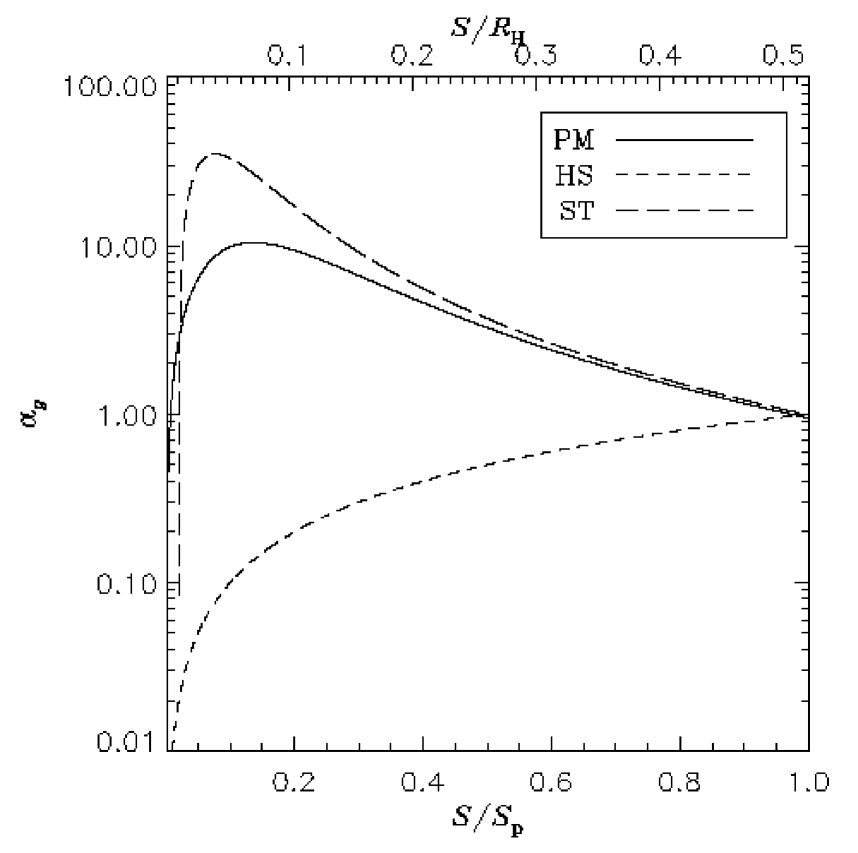
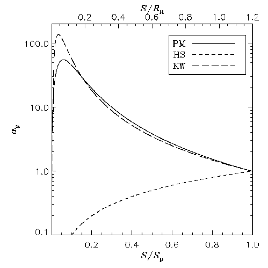
Figure 1: Left panel. Gravitational acceleration ($-\partial\Phi_{\mathrm{p}}/\partial S$) inside a $20\,M_{\oplus}$ planet as generated by the three potential functions $\Phi^{\mathrm{PM}}_{\mathrm{p}}$, $\Phi^{\mathrm{HS}}_{\mathrm{p}}$, and $\Phi^{\mathrm{ST}}_{\mathrm{p}}$ (eqs. [4], [6], and [7], respectively). Accelerations are normalized to $-G\,M_{\mathrm{p}}/S_{\mathrm{p}}^{2}$, where $S_{\mathrm{p}}$ is the envelope radius. The core mass (see § 2.1.2) is $15\,M_{\oplus}$ while $S_{\mathrm{p}}=0.52\,R_{\mathrm{H}}$. The core is supposed to have a density of $5.5\;\mbox{$\mathrm{g}\,\mathrm{cm}^{\mathrm{-3}}$}$. The point-mass potential is smoothed over a length $\varepsilon=0.1\,R_{\mathrm{H}}$ whereas in the Stevenson’s potential $\delta=5\times 10^{-2}\,R_{\mathrm{H}}$. Right panel. The same quantity is displayed inside a $90\,M_{\oplus}$ planet but this time involving the potential solution $\Phi^{\mathrm{KW}}_{\mathrm{p}}$ (eq. [9]). The adiabatic exponent is $\Gamma=1.43$ while the core mass is $60\,M_{\oplus}$. In all circumstances, the gravitational potential outside the envelope radius is of the type given in equation (4).

2.1.1 Homogeneous Sphere Solution

The gravitational potential generated by a homogeneous spherical distribution of matter can be calculated in a straightforward way by a direct integration of the gravitational force. Thereby, one finds

$$\Phi^{\mathrm{HS}}_{\mathrm{p}}=\left\{\begin{array}[]{ll}-\frac{G\,M_{\mathrm{p}}}{2\,S_{\mathrm{p}}}\left[3-\left(\frac{S}{S_{\mathrm{p}}}\right)^{2}\right]&\,\mathrm{if}\,S\leq S_{\mathrm{p}}\\ &\\ -\frac{G\,M_{\mathrm{p}}}{S}&\,\mathrm{if}\,S>S_{\mathrm{p}}\end{array},\right.$$ (6)

where $S_{\mathrm{p}}$ is the radius of the sphere, i.e., the planet’s radius. No smoothing is needed in this case since the force converges linearly to zero as the distance $S$ approaches zero. Thus, there is no risk of numerical instabilities.

Strictly speaking, equation (6) is valid inside very extended and nearly homogeneous envelopes without considerable cores. Then, one may think of the functions $\Phi^{\mathrm{PM}}_{\mathrm{p}}$ and $\Phi^{\mathrm{HS}}_{\mathrm{p}}$ as rendering two opposite extreme situations. Though $\Phi^{\mathrm{HS}}_{\mathrm{p}}$ does not represent a very realistic scenario of planet formation, for the sake of comparison and completeness, we will apply this potential to high- as well as low-mass bodies.

2.1.2 Stevenson’s Solution

Stevenson (1982) proposed a simplified analytical model of protoplanets having envelopes with constant opacity and surrounding an accreting solid core. He developed a radiative zero solution for hydrostatic and fully radiative spherical envelopes, which implies that both hydrostatic and thermal equilibrium are assumed inside the planet’s atmosphere. Under these hypotheses, the core can grow up to a critical mass whose value is that beyond which at least one of the two equilibriums ceases to exist (see discussion in Wuchterl, 1991) and the structure cannot be strictly static any longer. The critical core mass also sets an upper limit to the envelope and total mass of the planet. It can be proved that, at this critical point, $M_{\mathrm{c}}/M_{\mathrm{p}}=3/4$, where the mass of the core $M_{\mathrm{c}}$ is influenced by neither the nebula density nor its temperature.

The potential of the gravitational field established by a fully radiative envelope can be obtained from the density profile (see Stevenson, 1982) by applying the Poisson equation. Since the solid core size is by far below the resolution limit of these computations, the form of the Stevenson’s potential can be cast in the form

$$\Phi^{\mathrm{ST}}_{\mathrm{p}}=\left\{\begin{array}[]{ll}-\frac{G\,M_{\mathrm{c}}}{\sqrt{S^{2}+\delta^{2}}}-\frac{G\,M_{\mathrm{e}}^{{\dagger}}}{\sqrt{S^{2}+\delta^{2}}}&\\ &\\ \times\left[1-\left(\frac{S}{S_{\mathrm{p}}}\right)+\ln{\left(\frac{S}{S_{\textrm{c}}}\right)}\right]&\,\mathrm{if}\,S\leq S_{\mathrm{p}}\\ &\\ -\frac{G\,M_{\mathrm{p}}}{\sqrt{S^{2}+\delta^{2}}}&\,\mathrm{if}\,S>S_{\mathrm{p}}\end{array}.\right.$$ (7)

In equation (7) we have indicated with $S_{\mathrm{c}}$ the core radius. The quantity $M_{\mathrm{e}}^{{\dagger}}$ is equal to the planet’s envelope mass $M_{\mathrm{e}}=M_{\mathrm{p}}-M_{\mathrm{c}}$ divided by $\ln(S_{\mathrm{p}}/S_{\textrm{c}})$. The presence of the parameter $\delta$, also in the solution valid outside the envelope, is necessary for continuity reasons at $S=S_{\mathrm{p}}$. In these simulations we set $\delta=0.05\,R_{\mathrm{H}}$.

If the core has a density $\rho_{\mathrm{c}}=5.5\;\mbox{$\mathrm{g}\,\mathrm{cm}^{\mathrm{-3}}$}$ and accretes at the rate of $5\times 10^{-7}\;M_{\oplus}\,\mathrm{yr}^{\mathrm{-1}}$, assuming an envelope opacity equal to $1\;\mathrm{cm}^{2}\,\mathrm{g}^{-1}$ and a mean molecular weight of $2.2$, the critical total mass is $36\;M_{\oplus}$. Hence we will use equation (7) only for protoplanets whose total mass $M_{\mathrm{p}}$ is less than that value. Furthermore, we will suppose that the ratio of the total planetary mass to the core mass is the critical one. Therefore the core mass is always known once the mass $M_{\mathrm{p}}$ is assigned a value. Then, supplying $\rho_{\mathrm{c}}$, the radius $S_{\mathrm{c}}$ can be fixed.

The effects caused by equation (7) are actually similar to those caused by equation (4), as seen in Figure 1. In a more formal way, inside of the sphere $S=S_{\mathrm{p}}$, the normalized difference $\mathcal{R}^{\mathrm{ST}}$ between the two gravitational fields can be quantified by the ratio of $\left|\partial\Phi^{\mathrm{ST}}_{\mathrm{p}}/\partial S-\partial\Phi^{\mathrm{PM}}_{\mathrm{p}}/\partial S\right|$ to $\partial\Phi^{\mathrm{PM}}_{\mathrm{p}}/\partial S$, that is

$$\mathcal{R}^{\mathrm{ST}} = \frac{1}{4\,\ln(S_{\mathrm{p}}/S_{\textrm{c}})}$$ (8)

$$\times \left[\!\left(\frac{\delta}{S}\right)^{2}\!-\left(\frac{\delta}{S_{\mathrm{p}}}\right)\!\!\left(\frac{\delta}{S}\right)+\ln\!\left(\frac{S_{\mathrm{p}}}{S}\right)\!\right].$$

In the above relation, the equality $\varepsilon=\delta$ was imposed. $\mathcal{R}^{\mathrm{ST}}$ is a decreasing function of $S$. Referring to the models addressed in the left panel of Figure 1, $\mathcal{R}^{\mathrm{ST}}\simeq 5\%$ at $S/S_{\mathrm{p}}=1/3$. This result is only slightly affected by the mass of the planet because $S_{\mathrm{p}}$ is a slowly varying function of $M_{\mathrm{p}}$.

2.1.3 Wuchterl’s Solution

Along with the fully radiative envelope, other static solutions were found. Following the track of Stevenson’s arguments, Wuchterl (1993) developed an analytical model for protoplanets with spherically symmetric and fully convective envelopes. In this case the hydrostatic structure is determined by the constant entropy requirement that is appropriate when convection is very efficient. Supposing that the adiabatic exponent $\Gamma=d\ln{p}/d\ln{\rho}$ is constant throughout the envelope, integrating the envelope density one finds that a solution for the planet gravitational potential is

$$\Phi^{\mathrm{KW}}_{\mathrm{p}}=\left\{\begin{array}[]{ll}-\frac{G\,M_{\mathrm{c}}}{\sqrt{S^{2}+\delta^{2}}}-\frac{G\,M_{\mathrm{e}}^{{\ddagger}}}{\sqrt{S^{2}+\delta^{2}}}&\\ &\\ \times\left[\left(\frac{\zeta}{\zeta-1}\right)\!\!\left(\frac{S}{S_{\mathrm{p}}^{\Gamma}}\right)\!\!-\left(\frac{1}{\zeta-1}\right)\!\!\left(\frac{S}{S_{\mathrm{p}}^{\Gamma}}\right)^{\zeta}-\Pi\right]&\\ &\\ \quad\quad\quad\quad\quad\mathrm{if}\,S\leq S_{\mathrm{p}}^{\Gamma}&\\ &\\ -\frac{G\,M_{\mathrm{p}}}{\sqrt{S^{2}+\delta^{2}}}\quad\mathrm{if}\,S>S_{\mathrm{p}}^{\Gamma}&\end{array},\right.$$ (9)

where we set $\zeta=(3\,\Gamma-4)/(\Gamma-1)$ and $\Pi=(S_{\mathrm{c}}/S_{\mathrm{p}}^{\Gamma})^{\zeta}$. Moreover, the envelope mass is written as $M_{\mathrm{e}}=(1-\Pi)\,M_{\mathrm{e}}^{{\ddagger}}$. The condition for stability of gas spheres ($\Gamma>4/3$) implies that $\zeta$ is positive. This particular form of $\Phi^{\mathrm{KW}}_{\mathrm{p}}$ is obtained by choosing an envelope radius equal to $S_{\mathrm{p}}^{\Gamma}=(\Gamma-1)\,R_{\mathrm{ac}}$. The length $R_{\mathrm{ac}}=G\,M_{\mathrm{p}}/c^{2}_{\mathrm{s}}$ is called “planetary accretion radius”. Outside the sphere $S=R_{\mathrm{ac}}$ the thermal energy of the gas is higher than the gravitational energy binding it to the planet.

As in Stevenson’s solution, critical mass values exist for the envelope structure to be static. However, unlike the fully radiative envelope case, now the critical core mass depends on both the temperature and the density of ambient material. Furthermore, the critical mass ratio is $M_{\mathrm{c}}/M_{\mathrm{p}}=2/3$ (for details see Wuchterl, 1993). Setting $\Gamma$ to $1.43$ and the mean molecular weight to $2.2$, if nebula conditions are $T_{\mathrm{Neb}}=100\;\mathrm{K}$ and $\rho_{\mathrm{Neb}}=10^{-10}\;\mbox{$\mathrm{g}\,\mathrm{cm}^{\mathrm{-3}}$}$, the critical total mass is $M_{\mathrm{p}}=274\;M_{\oplus}$.

Wuchterl’s solution well applies to massive protoplanets since they are likely to bear convective envelopes.

Concerning the differences between equation (9) and equation (4), the situation is alike to that met in § 2.1.2 (see right panel of Fig. 1). In this circumstance, for $S\leq S_{\mathrm{p}}$, the normalized difference can be written as

$$\mathcal{R}^{\mathrm{KW}} = \left(\frac{1}{3}\right)\!\!\frac{1}{1-\Pi}\!\left\{1\!+\!\left(\frac{\zeta}{\zeta-1}\right)\!\!\left(\frac{\delta}{S_{\mathrm{p}}}\right)\!\!\left(\frac{\delta}{S}\right)\right.$$ (10)

$$\times \left.\left[1-\left(\frac{S}{S_{\mathrm{p}}}\right)^{\zeta-1}\right]-\left(\frac{S}{S_{\mathrm{p}}}\right)^{\zeta}\right\}.$$

As before, the equality $\varepsilon=\delta$ is assumed and $\mathcal{R}^{\mathrm{KW}}$ decreases with $S$. Using the parameters adopted for the models illustrated in the right panel of Figure 1, $\mathcal{R}^{\mathrm{KW}}\simeq 18\%$ at $S/S_{\mathrm{p}}=1/3$. In the considered range of masses, this number is nearly constant. In fact, equation (10) can be approximated to

$$\mathcal{R}^{\mathrm{KW}}\approx\left(\frac{1}{3}\right)\left[1-\left(\frac{S}{S_{\mathrm{p}}}\right)^{\zeta}\right].$$ (11)

2.2 Physical Parameters

Table 1: Planetary Masses and Adopted Gravitational Potential.

$M_{\mathrm{p}}\tablenotemark{a}\;/M_{\oplus}$	$q$	$S_{\mathrm{p}}/R_{\mathrm{H}}$	$R_{\mathrm{H}}/a$	Potential
333string	$1.00\times 10^{-3}$	$0.87$	$6.9\times 10^{-2}$	PM, HS
253string	$7.56\times 10^{-4}$	$2.30$	$6.3\times 10^{-2}$	KW
166string	$5.00\times 10^{-4}$	$0.78$, $1.70$	$5.5\times 10^{-2}$	PM, KW, HS
093string	$2.83\times 10^{-4}$	$1.20$	$4.5\times 10^{-2}$	KW
067string	$2.00\times 10^{-4}$	$0.70$, $0.96$	$4.0\times 10^{-2}$	PM, KW
033string	$1.00\times 10^{-4}$	$0.60$	$3.2\times 10^{-2}$	PM, HS
029string	$8.80\times 10^{-5}$	$0.58$	$3.1\times 10^{-2}$	ST
020string	$6.00\times 10^{-5}$	$0.52$	$2.7\times 10^{-2}$	HS, ST
015string	$4.50\times 10^{-5}$	$0.46$	$2.5\times 10^{-2}$	ST
012.5	$3.75\times 10^{-5}$	$0.44$	$2.3\times 10^{-2}$	ST
010string	$3.00\times 10^{-5}$	$0.38$	$2.1\times 10^{-2}$	PM, HS, ST
007string	$2.10\times 10^{-5}$	$0.34$	$1.9\times 10^{-2}$	ST
005string	$1.50\times 10^{-5}$	$0.29$	$1.7\times 10^{-2}$	HS, ST
003string	$1.00\times 10^{-5}$	$0.23$	$1.5\times 10^{-2}$	ST
001.5	$4.50\times 10^{-6}$	$0.16$	$1.1\times 10^{-2}$	ST

Note. — List of all the simulated planet masses: $q=M_{\mathrm{p}}/M_{\bigstar}$ is the non-dimensional quantity that enters the simulation. Note that $M_{\mathrm{p}}=333\;M_{\oplus}=1.05\;M_{\jupiter}$. The ratio $R_{\mathrm{H}}/a$ is equal to $\left(q/3\right)^{1/3}$ (see § 2.1). Unless stated otherwise, envelope radii $S_{\mathrm{p}}$ are expressed through a combination of the Hill ($R_{\mathrm{H}}$) and the accretion ($R_{\mathrm{ac}}$) radius of the planet, as plotted in Figure 2 (courtesy of P. Bodenheimer). When required, we set $M_{\mathrm{c}}=(2/3)\,M_{\mathrm{p}}$ for a fully convective envelope and $M_{\mathrm{c}}=(3/4)\,M_{\mathrm{p}}$ for a fully radiative one. The core radius is computed assuming a constant density $\rho_{\mathrm{c}}=5.5\;\mbox{$\mathrm{g}\,\mathrm{cm}^{\mathrm{-3}}$}$ in both cases.

We consider a protostellar disk orbiting a one solar-mass star. The simulated region extends for $2\,\pi$ around the polar axis and, radially, from $2.08$ to $13\;\mbox{{AU}}$. The aspect ratio is fixed to $h=0.05$ throughout these computations. As in Paper I, the disk is assumed to be symmetric with respect to its midplane. This allows us to reduce the latitude range to the northern hemisphere only, where $\theta$ varies between $80\arcdeg$ and $90\arcdeg$. The co-latitude interval includes $3.5$ disk scale-heights and therefore it assures a vertical density drop of more than six orders of magnitude (see § 3.3). The mass enclosed within this domain is $M_{\mathrm{D}}=3.5\times 10^{-3}\;M_{\odot}$, which implies, in our case, that a mass equal to $0.01\;M_{\odot}$ is confined inside $26\;\mbox{{AU}}$. Disk material is supposed to have a constant kinematic viscosity $\nu=10^{15}\;\mathrm{cm}^{2}\,\mathrm{s}^{-1}$, corresponding to $\alpha=4\times 10^{-3}$ at the planet’s location.

The orbital radius of the planet is $R_{\mathrm{p}}=5.2\;\mbox{{AU}}$ and its azimuthal position is fixed to $\varphi=\varphi_{\mathrm{p}}=\pi$. We concentrate on a mass range stretching from $1.5\;M_{\oplus}$ to one Jupiter-mass ($M_{\jupiter}$), implying that the mass ratio $q=M_{\mathrm{p}}/M_{\bigstar}\in[4.5\times 10^{-6},10^{-3}]$, if $M_{\bigstar}=1\;M_{\odot}$. A detailed list of the examined planetary masses, along with the adopted potential form is given in Table 1.

The choice of few of the above parameters represents one typical example during the early phase of planet formation. Additionally, these simulations offer the good advantage that the system of equations is cast in a non-dimensional form, thus all of the outcomes are “scale-free” with respect to $M_{\bigstar}$, $M_{\mathrm{D}}$, and $R_{\mathrm{p}}$.

Figure 2: Envelope radius $S_{\mathrm{p}}$, as provided by P. Bodenheimer (2001, private communication), compared to the Hill radius $R_{\mathrm{H}}$ and the accretion radius $R_{\mathrm{acc}}$. In a locally isothermal disk with aspect ratio $h$, $R_{\mathrm{H}}$ is larger than $R_{\mathrm{ac}}$ when $q<h^{3}/\sqrt{3}$. While the scale of the left vertical axis is referred to orbital radius $R_{\mathrm{p}}=5.2\;\mbox{{AU}}$, the scale on the right one is compared to the radius of Jupiter $R_{\jupiter}=7.1\times 10^{4}\;\mathrm{km}$.

According to studies of the early evolution of protoplanets, the Roche lobe is usually filled during the growth phase. In such calculations the envelope is allowed to extend to either the Hill radius $R_{\mathrm{H}}$ or the accretion radius $R_{\mathrm{ac}}$ (Bodenheimer & Pollack, 1986; Wuchterl, 1991; Tajima & Nakagawa, 1997). Except for Wuchterl’s solution, where we set $S_{\mathrm{p}}=S_{\mathrm{p}}^{\Gamma}=(\Gamma-1)\,R_{\mathrm{ac}}$, the estimates of planet radii used in the simulations were provided by P. Bodenheimer (2001, private communication). They originate from a combination of $R_{\mathrm{H}}$ and $R_{\mathrm{ac}}$ at an ambient temperature of $T=100\;\mathrm{K}$ (see Fig. 2). The values of $S_{\mathrm{p}}$, employed in each model, are also reported in Table 1.

It is worthwhile to stress that the planetary (or more properly, the envelope) radius $S_{\mathrm{p}}$ does not represent any real physical boundary but only the distance beyond which the planet’s potential reduces to the one given in equation (4), i.e., to a point-mass potential.

3 Numerical Issues

The set of hydrodynamic equations that characterizes the temporal evolution of a disk-planet system is solved numerically by means of a finite difference scheme provided by an early FORTRAN-coded version of Nirvana (Ziegler & Yorke, 1997; Ziegler, 1998). The code has been modified and adapted to our purposes as described in Paper I, Paper II, and references therein. In order to investigate thoroughly the flow dynamics in the neighborhood of the planet, a sufficient numerical resolution is required. We accomplish that by employing a nested-grid strategy. This can be pictured as either a set of grids, each hosting an inner one, or a pyramid of levels: the main grid (level one) includes the whole computational domain, while inner grids (higher levels) enclose smaller volumes around the planet, with increasing resolution. Levels greater than one are also called subgrids since they are usually smaller in size. The linear resolution, in each direction, doubles when passing from a grid to the inner one.

The basic principles upon which the nested-grid technique relies and how it is applied to disk-planet simulations in two dimensions is explained in detail in Paper II and references therein. The extension to the three-dimensional geometry, though requiring some more complexity in the exchange of information from one grid level to the neighboring ones, is nearly straightforward. Coarse-fine grid interaction (which sets the boundary conditions necessary for the integration of subgrids) is accomplished via a direction-splitting procedure. Thus, with respect to the discussion in Paper II, the addition of a third dimension just requires the implementation of the third direction-splitting step in the algorithm. Fine-coarse grid interaction (which upgrades the solution on finer resolution regions) involves, in 3D, volume-weighted averages in a spherical polar topology. These are given in the Appendix.

3.1 General Setup

Table 2: Grid Hierarchies Utilized in the Simulations.

Grid	Main Grid Size	$ng$	Subgrid Size	No. of models
G0	$121\times 13\times 319$	4	$54\times 12\times 48$	10
G1	$143\times 13\times 423$	4	$64\times 12\times 64$	05
G2	$121\times 13\times 319$	5	$54\times 12\times 48$	19
G3	$143\times 13\times 423$	5	$64\times 12\times 64$	12
G4	$121\times 23\times 319$	5	$54\times 22\times 48$	04
G5	$133\times 13\times 395$	5	$84\times 16\times 84$	01

Note. — Grid sizes are reported as the number of grid points per direction: $N_{R}\times N_{\theta}\times N_{\varphi}$. The third column ($ng$) indicates the number of levels within the hierarchy. In order to achieve sufficient resolution within the Roche lobe of the planet, grids G0 and G1 have been used only for planetary masses in the range $[67\;M_{\oplus},1\;M_{\jupiter}]$. Grids are ordered according to their computing time requirements, which grow from top to bottom. The hierarchy G5 has been employed to execute the model with $M_{\mathrm{p}}=12.5\;M_{\oplus}$ (see discussion at the end of § 4.2).

For the study of the variety of planetary masses indicated in Table 1, meeting both the requirements of high resolution and affordable computing times, we realized a series of six grid hierarchies, whose characteristics are given in Table 2. With mass ratios $q$ larger than $2\times 10^{-4}$ ($67\;M_{\oplus}$) only grids G0 and G1 are utilized whereas smaller bodies are investigated with the other grid hierarchies. Thereupon, the finest resolution we obtain in the whole set of simulations varies form $0.03$ to $0.06\,R_{\mathrm{H}}$. In all of the models presented here, the planet is centered at the corner of a main grid cell, which property is retained on any higher hosted subgrid. As the planet radial distance is $R_{\mathrm{p}}=a/(1+q)$, we adjust it by tuning the value of the star-planet distance $a$. Adjustments never exceed 0.7% over the nominal value of $R_{\mathrm{p}}$ given in § 2.2. Every model is evolved at least till 200 orbits. The evolution of massive planets ($M_{\mathrm{p}}\geq 67\;M_{\oplus}$) is followed for 300 to 400 orbital periods because they take longer to settle on a quasi-stationary state.

Gas accretion is estimated following the procedure sketched in Paper II. For better accuracy, mass is removed only from the finest grid level according to an accretion sphere radius $\kappa_{\mathrm{ac}}$ and an evacuation parameter $\kappa_{\mathrm{ev}}$. The former defines the spherical volume which contributes to the accretion process whereas the latter can be regarded as a measure of the removal time scale in such volume. Two-dimensional simulations showed that the procedure is fairly stable against these two parameters. We constrain the amount of removed mass per unit volume not to exceed 1% of that available, as was done in Paper II. Regarding the extension of the sphere of accretion $\kappa_{\mathrm{ac}}$, we performed simulations using different values, as stated in Table 3. Since the planet actually works as a sink, our procedure only furnishes upper limits to realistic planetary accretion rates (see discussion in Tanigawa & Watanabe, 2002).

However, we also inquire how mass removal can possibly affect gravitational torques and, more generally, the dynamics of the flow in the planet neighborhood by means of models in which accretion is prohibited.

Table 3: Mass Accretion Parameter $\kappa_{\mathrm{ac}}$.

$M_{\mathrm{p}}/M_{\oplus}$	$q$	$\kappa_{\mathrm{ac}}/R_{\mathrm{H}}$	Accreting Only
333string	$1.00\times 10^{-3}$	$0.20$, $0.15$, $0.10$	No
253string	$7.60\times 10^{-4}$	$0.10$	Yes
166string	$5.00\times 10^{-4}$	$0.10$	Yes
093string	$2.80\times 10^{-4}$	$0.10$	Yes
067string	$2.00\times 10^{-4}$	$0.20$, $0.10$	No
033string	$1.00\times 10^{-4}$	$0.20$, $0.10$	No
029string	$8.80\times 10^{-5}$	$0.20$, $0.10$	No
020string	$6.00\times 10^{-5}$	$0.15$, $0.10$	No
015string	$4.50\times 10^{-5}$	$0.10$	Yes
012.5	$3.75\times 10^{-5}$	$0.10$	Yes
010string	$3.00\times 10^{-5}$	$0.10$	No
007string	$2.10\times 10^{-5}$	$0.10$	Yes
005string	$1.50\times 10^{-5}$	$0.10$	No
003string	$1.00\times 10^{-5}$	$0.10$	Yes
001.5	$4.50\times 10^{-6}$	$0.07$	Yes

Note. — The parameter $\kappa_{\mathrm{ac}}$ represents the radius of the accreting region. Within this sphere the mass density is reduced by roughly 1% after every time step. The length $\kappa_{\mathrm{ac}}=0.1\,R_{\mathrm{H}}$ should be small enough to make the accretion procedure almost independent of the evacuation parameter $\kappa_{\mathrm{ev}}$ (Tanigawa & Watanabe, 2002). At $q=3\times 10^{-5}$ ($M_{\mathrm{p}}=10\;M_{\oplus}$) a non-accreting simulation was performed with $\Phi_{\mathrm{p}}=\Phi^{\mathrm{HS}}_{\mathrm{p}}$ (eq. [6]) as well as with $\Phi_{\mathrm{p}}=\Phi^{\mathrm{ST}}_{\mathrm{p}}$ (eq. [7]). In the case of lowest mass model ($M_{\mathrm{p}}=1.5\;M_{\oplus}$), we allowed the ratio $\kappa_{\mathrm{ac}}/S_{\mathrm{p}}$ to be less than $0.5$, as in all of the other models. For a better evaluation of $\dot{M}_{\mathrm{p}}$, we used a modified version of the grid system G3 which contains a sixth level, comprising (approximately) the planet’s Hill sphere.

3.2 Boundary Conditions

In order to mimic the accretion of the flow towards the central star, an outflow boundary condition is applied at the inner radial border of the computational domain. The outer radial border is closed, i.e., no material can flow in or out of it. The same condition exists at the highest latitude $\theta=80\arcdeg$. Since the disk is symmetric with respect to its midplane as mentioned in § 2.2, symmetry conditions are set at $\theta=90\arcdeg$. On subgrids, except for the midplane where symmetry conditions are applied, boundary values are interpolated from hosting grids, by means of a monotonised second-order algorithm (see Paper II for details).

The open inner radial boundary causes the disk to slowly deplete during its evolution. For all the models under study, we observe a depletion rate $\dot{M}_{\mathrm{D}}=-\dot{M}_{\bigstar}$ measuring $\approx 10^{-8}\;\mbox{$M_{\odot}\,\mathrm{yr}^{\mathrm{-1}}$}$, in agreement with the expectations of stationary Keplerian disks: $\dot{M}_{\bigstar}=3\,\pi\,\nu\,\Sigma$ (Lynden-Bell & Pringle, 1974).

In cases of gap formation, material residing inside the planet’s orbit tends to drain out of the computational domain. Since this material transfers angular momentum to the planet, the lack of it may contribute to reduce both the migration time scale and the planet’s accretion rate. To evaluate these effects, a Jupiter-mass model was run with a closed (i.e., reflective) inner radial border.

3.3 Initial Conditions

The initial density distribution is a power-law of the distance from the rotational axis $r=R\,\sin{\theta}$ times a Gaussian in the vertical direction

$$\rho(t=0)=\rho_{0}(r)\,\exp\left[-\left(\frac{\cot\theta}{h}\right)^{2}\right],$$ (12)

which is appropriate for a thin disk in thermal and hydrostatic vertical equilibrium. The dependency of the midplane value $\rho_{0}$ with respect to $r$ is such that the initial surface density profile $\Sigma$ decays as $1/\sqrt{r}$, as required by the constant kinematic viscosity. However, we also ran a few models where the relation $\rho_{0}(r)$ is such to account for an axisymmetric gap, as often done to speed up the computations at early evolutionary times.

The initial velocity field of the fluid is a purely, counter-clockwise, Keplerian one corrected by the grid rotation: $\boldsymbol{u}(t=0)\equiv(0,0,v_{K}-\Omega_{\mathrm{p}}\,r)$. Thus, the partial support due to the radial pressure gradient is neglected in the beginning.

4 Simulation Results

4.1 Flow Dynamics near Protoplanets

Two-dimensional computations have shown that a circumplanetary disk forms around Jupiter-type planets, extending over the size of its Roche lobe (Kley, 1999; Lubow, Seibert, & Artymowicz, 1999; Tanigawa & Watanabe, 2002). The numerical experiments conducted in Paper II proved this characteristic to belong not only to massive bodies but also to protoplanets as small as $3\;M_{\oplus}$. The authors demonstrated that the flow of such disks is approximately Keplerian down to distances $\sim 0.1\,R_{\mathrm{H}}$ from the planet. One of the main features of these disks is a two-arm spiral shock wave whose opening angle (that between the wave front and the direction toward the planet) is an increasing function of the mass ratio $q$ and, below $M_{\mathrm{p}}=67\;M_{\oplus}$, it is roughly given by $\arctan(\mathcal{M})$, in which $\mathcal{M}=|\boldsymbol{u}|/c_{\mathrm{s}}$ is the Mach number of the circumplanetary flow (D’Angelo, Kley, & Henning, 2002). The spiral patterns shorten and straighten as the perturber mass decreases. Eventually, for even smaller masses they disappear and are not observable anymore when one Earth-mass is reached.

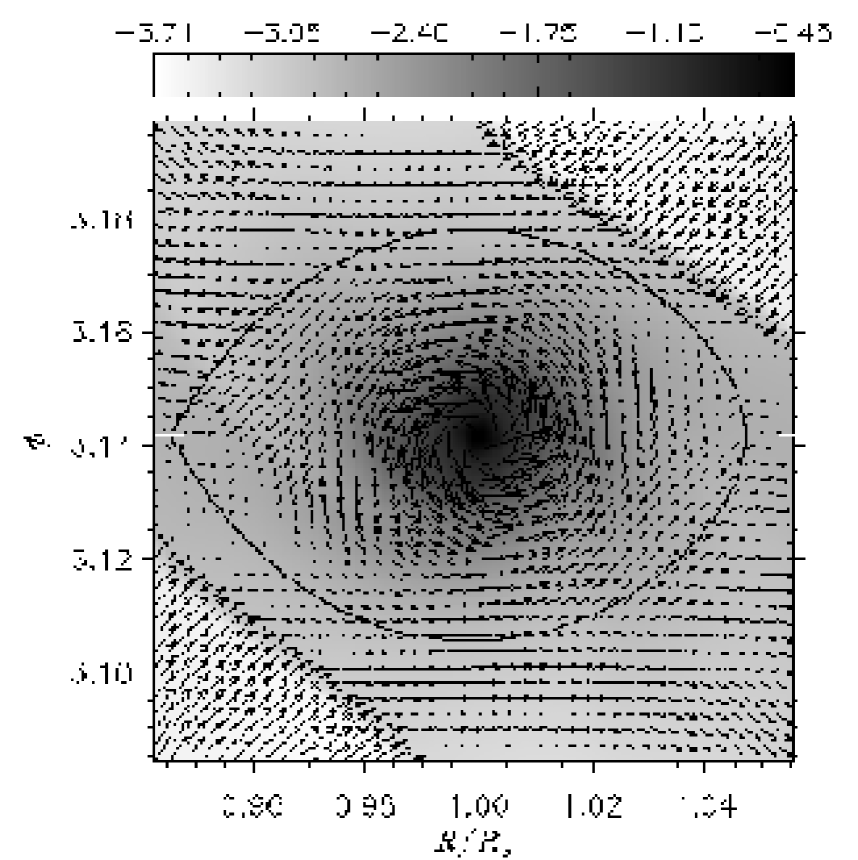
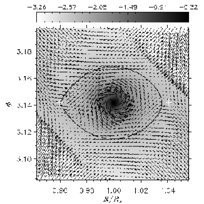
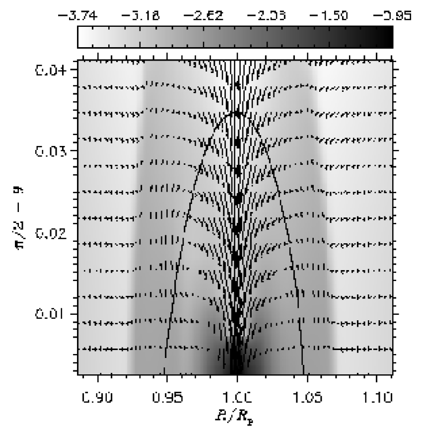
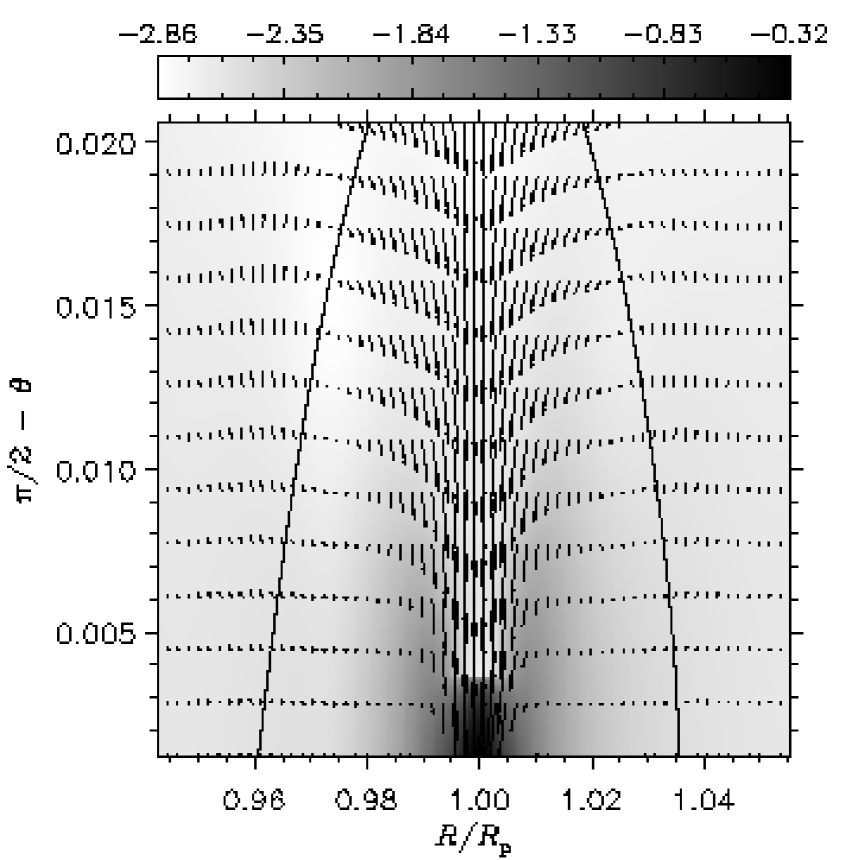
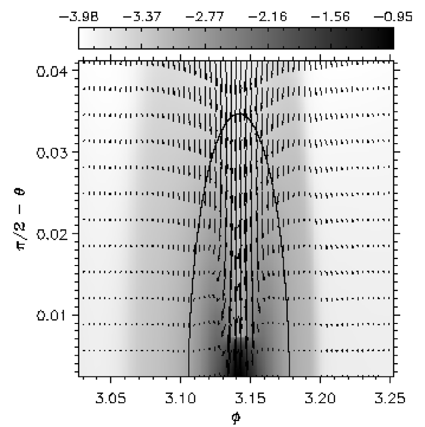
Figure 3: Density slices with an overplotted two-component velocity field. In order to comprise the whole density range, the color scale represents the logarithm of the density ($\log{\rho}$). The evolutionary time is 200 orbital periods. Slices are cut at the planet location: $\theta=\pi/2$ (top), $\varphi=\varphi_{\mathrm{p}}$ (middle), and $R=R_{\mathrm{p}}$ (bottom). Both models are accreting and executed with Wuchterl’s potential. In physical units, $\rho=10^{-2}$ is equivalent to $4.22\times 10^{-11}\;\mbox{$\mathrm{g}\,\mathrm{cm}^{\mathrm{-3}}$}$. Left panels. Planet with a total mass $M_{\mathrm{p}}=166\;M_{\oplus}$ and a core mass equal to $2/3\,M_{\mathrm{p}}$ (critical core mass). Right panels. Planet with $M_{\mathrm{p}}=67\;M_{\oplus}$ and a critical core mass. The curve drawn in each panel indicates the trace of the Roche lobe. In the left and right top panels, the flow reaches velocities equal to $\sim 3$ and $\sim 2\;\mathrm{km}\,\mathrm{s}^{-1}$, respectively. In the other panels, maximum velocities are on the order of $\sim 4\;\mathrm{km}\,\mathrm{s}^{-1}$.

Three-dimensional simulations shed new light on these circumplanetary disks, demonstrating that they can behave somehow differently from what depicted by two-dimensional descriptions. Differences become more marked as the mass of the embedded protoplanet is lowered. A major point is that spiral waves are not so predominant as they are in the 2D geometry. This is clearly seen in the top rows of Figure 3 and 4, where the midplane ($\theta=\pi/2$) density is displayed for four different planetary masses. The double pattern of the spiral is still visible around a $67\;M_{\oplus}$ protoplanet (Fig. 3, top right panel). However, when considering a planet half of that size, spiral traces are too feeble to be seen on the image (Fig. 4, top left panel). Such an occurrence was to be expected since the energy of the flow is not only converted into the equatorial motion but can be also transferred to the vertical motion of the fluid. It was already known from wave theories for circumstellar disks (Lubow, 1981; Lubow & Pringle, 1993; Ogilvie & Lubow, 1999) and related numerical calculations (Makita, Miyawaki, & Matsuda, 2000) that the three-dimensional propagation of spiral perturbations may be significantly different from that obtained in two dimensions because of the existence of vertical resonances. Furthermore, Miyoshi et al. (1999) already noticed in their shearing sheet models the weakening effect of the finite disk thickness upon the formation of spiral waves around embedded protoplanets. Hence, we may argue that the averaging of the pressure and the gravitational potential, which is accomplished in an infinitesimally thin disk, enhances spiral features in disks.

The remainder of this section is devoted to a general description of the vertical circulation of the material in the vicinity of the planet. We start inspecting what happens in the slice $\varphi=\varphi_{\mathrm{p}}$, i.e., in the $R$–$\theta$ surface containing the planet (see middle panels in Fig. 3 and 4). The first thing to note is that the material above the equatorial plane moves toward the planet with a negligible meridional component, in fact $|u_{\theta}|\ll u$ (where $u=|\boldsymbol{u}|$). Therefore matter is nearly confined to $\theta$-constant surfaces. This circumstance favors the use of 2D outcomes as predictions of 3D expectations (Masset, 2002). However this turns out to be true only far away from the planet. In fact, as the fluid enters a certain region around the Hill sphere, its dynamics changes drastically. The beginning of this zone is marked by two shock fronts, which actually develop well outside the Roche lobe of the restricted three body problem. The distance of the shock fronts from the perturber, if compared to $R_{\mathrm{H}}$, shrinks from $2.61$ to $1.16$ as $M_{\mathrm{p}}$ is increased from $10\;M_{\oplus}$ to $1\;M_{\jupiter}$. Generally, shocks are not placed symmetrically with respect to the planet. Past these shocks, material is deflected upward and then it recirculates downward, while approaching the radial position of the planet (see middle panels in Fig. 3 and 4).

At $R\approx R_{\mathrm{p}}$, matter suffers an unbalanced gravitational attraction by the planet and accelerates downward towards it. Velocities are supersonic, reaching a Mach number $\mathcal{M}\simeq 8$, when $67\;M_{\oplus}\lesssim M_{\mathrm{p}}\leq 1\;M_{\jupiter}$, and $\mathcal{M}\simeq 2$ if $M_{\mathrm{p}}=20\;M_{\oplus}$. They become subsonic for planetary masses between $10$ and $1.5\;M_{\oplus}$, ranging from 30% to 5% of the local sound speed. Because of the sinking material, at $\theta=\pi/2$ the flow field is slightly horizontally divergent from the planet location.

As one can judge from Figure 4 (middle panels), the flow gets less and less symmetric, with respect to $R_{\mathrm{p}}$, as the planet mass is reduced. Recirculation persists before the planet ($R<R_{\mathrm{p}}$) but vanishes behind it ($R>R_{\mathrm{p}}$). Any symmetry disappears starting from $M_{\mathrm{p}}=5\;M_{\oplus}$ downwards.

Along the azimuthal direction (slice $R=R_{\mathrm{p}}$, i.e., in the surface $\varphi$–$\theta$ containing the planet), the bottom panels of Figure 3 and 4 show an even more complex situation. Below $166\;M_{\oplus}$, the region of influence of the planet appears to be more comparable in size with the Roche lobe. However, apart from that, the general behavior of the flow differs from case to case, having in common a rapid descending motion when the material lies above the planet. Around Jupiter-sized planets some kind of weak, non-closed, recirculation may be seen. This flow feature is still present at both sides of a $29\;M_{\oplus}$ planet (bottom left panel, Fig. 4), whereas it tends to vanish in models with lower $q$-ratios.

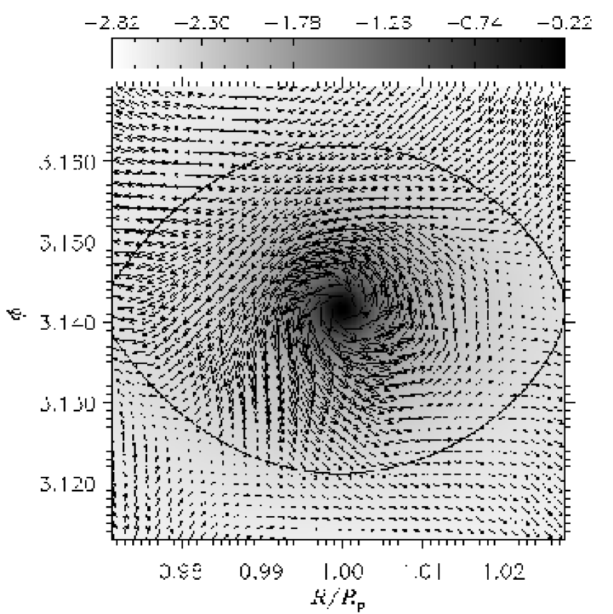
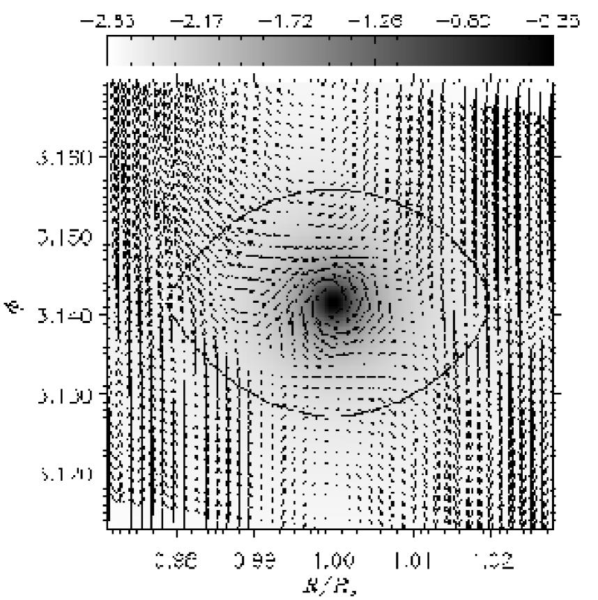
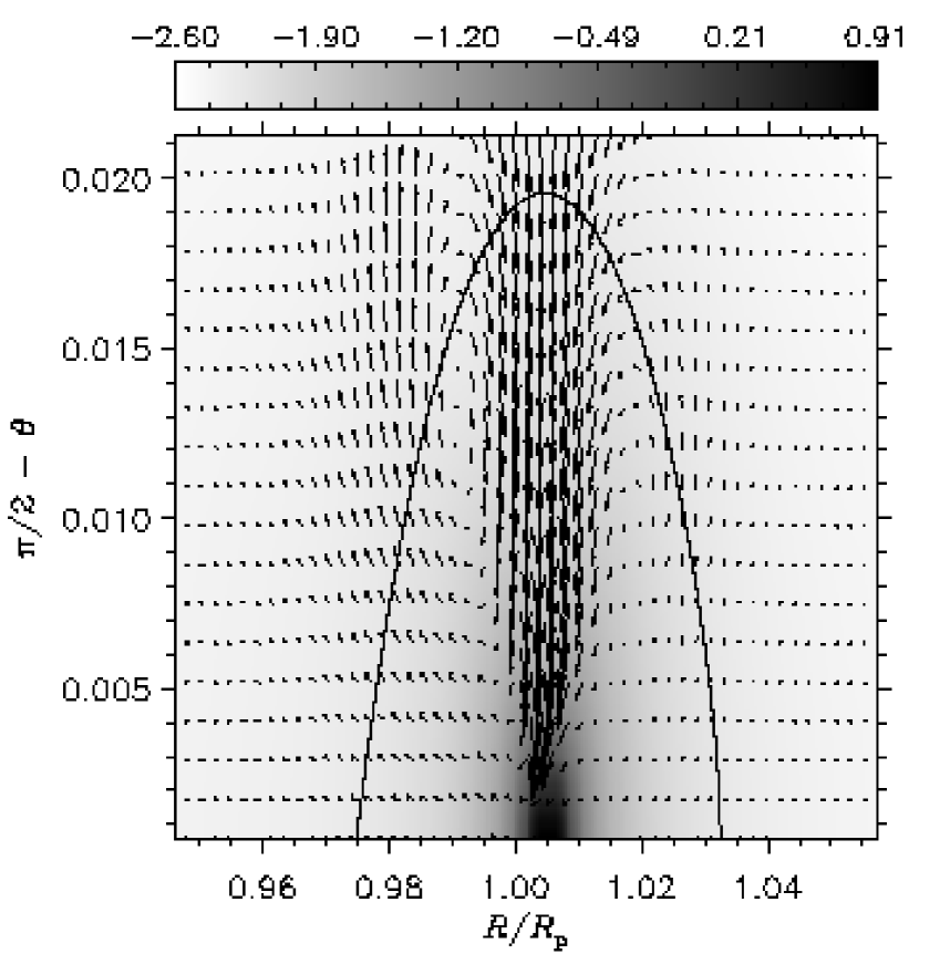
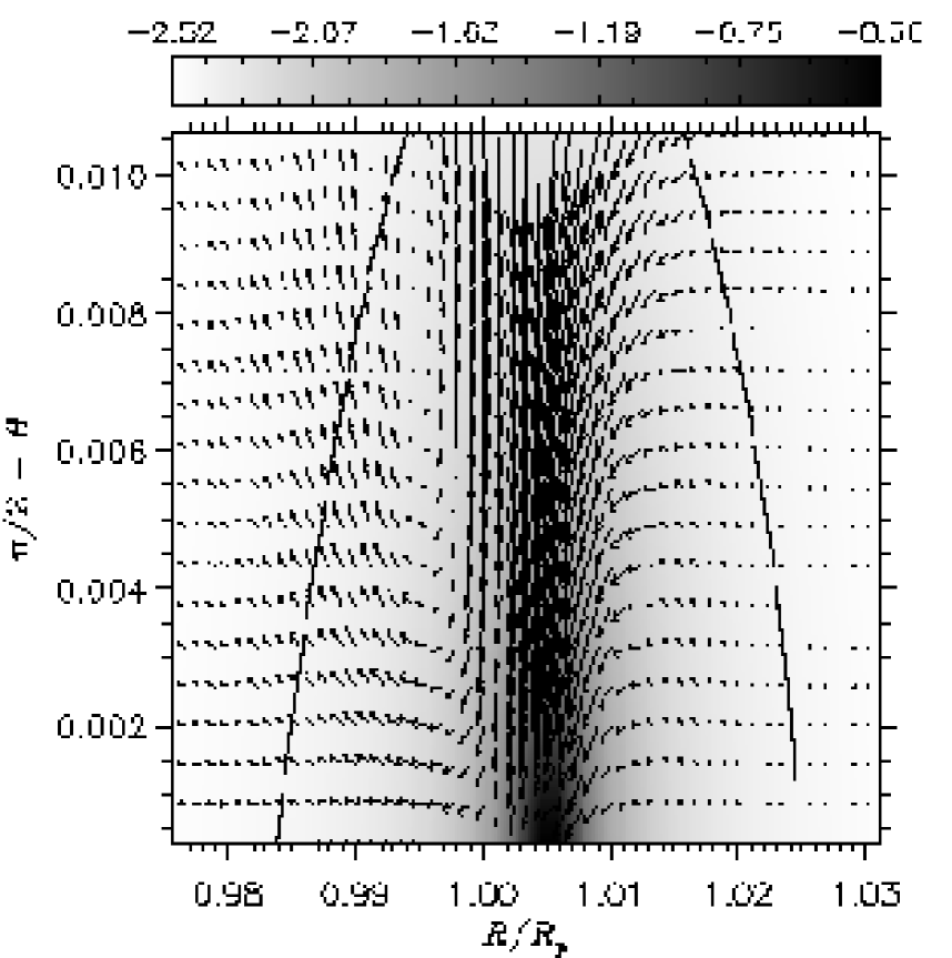
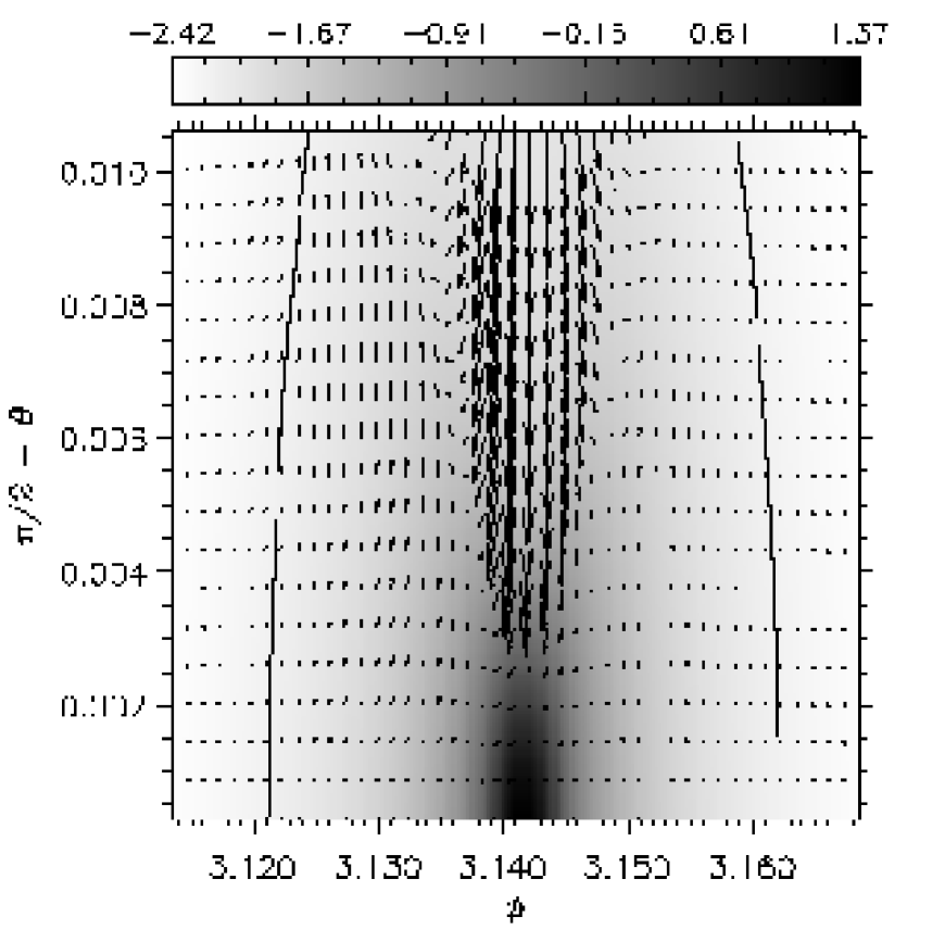
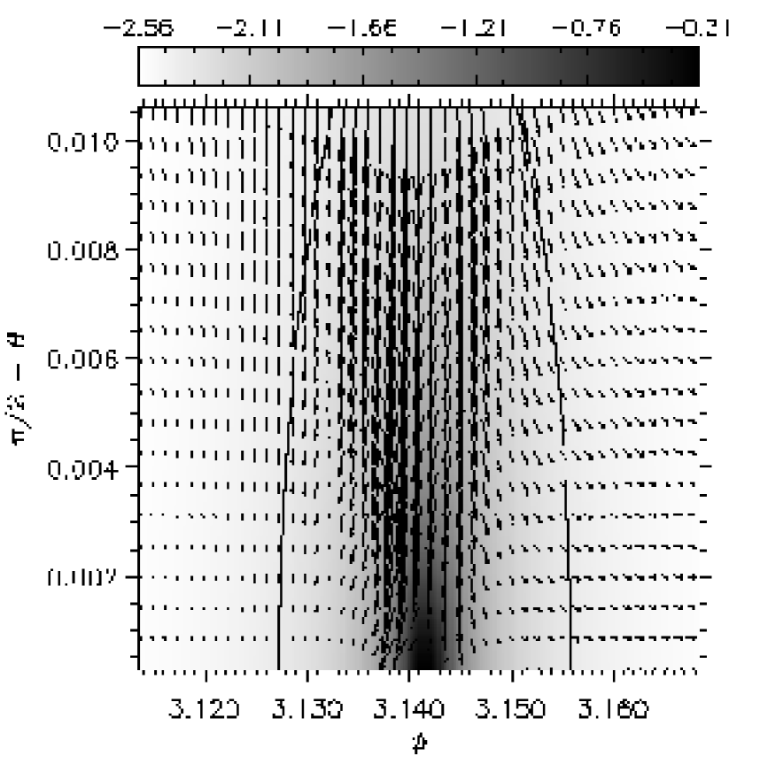
Figure 4: Density slices of the same type as in Figure 3, illustrating low-mass accreting planets after 200 orbits. In these simulations, Stevenson’s potential is employed. In physical units, the density scale is as in Figure 3. The density value $\rho=10^{-2}$ corresponds to $4.22\times 10^{-11}\;\mbox{$\mathrm{g}\,\mathrm{cm}^{\mathrm{-3}}$}$. Left panels. Planet with $M_{\mathrm{p}}=29\;M_{\oplus}$ and a critical core mass $M_{\mathrm{c}}=21.7\;M_{\oplus}$. Maximum flow speeds, within $S=R_{\mathrm{H}}$, are $\sim 1\;\mathrm{km}\,\mathrm{s}^{-1}$ in each of the three panels. Right panels. Planet with $M_{\mathrm{p}}=10\;M_{\oplus}$ and a core mass and $M_{\mathrm{c}}=7.5\;M_{\oplus}$. Inside of the Hill sphere, maximum velocities are on the order of $0.2\;\mathrm{km}\,\mathrm{s}^{-1}$.

4.1.1 Non-accreting Protoplanets

Table 4: Mass enclosed within the Envelope Radius.

		No Accretion			Accretion
$M_{\mathrm{p}}$		$\widehat{M}_{\mathrm{e}}$	$\widehat{\rho}_{\mathrm{e}}$		$\widehat{M}_{\mathrm{e}}$	$\widehat{M}_{\mathrm{e}}$	$\widehat{M}_{\mathrm{e}}$
67		$7.07\times 10^{-1}$	$9.37\times 10^{-11}$		$1.07\times 10^{-1}$	$\cdots$	$7.67\times 10^{-2}$
29		$2.74\times 10^{-1}$	$1.45\times 10^{-10}$		$6.49\times 10^{-2}$	$\cdots$	$\cdots$
20		$2.26\times 10^{-1}$	$2.43\times 10^{-10}$		$3.68\times 10^{-2}$	$3.18\times 10^{-2}$	$\cdots$
10		$1.29\times 10^{-2}$	$7.12\times 10^{-11}$		$9.76\times 10^{-3}$	$\cdots$	$\cdots$
05		$2.24\times 10^{-3}$	$5.56\times 10^{-11}$		$2.17\times 10^{-3}$	$\cdots$	$\cdots$

Note. — All masses are relative to the Earth’s mass. The mean density $\widehat{\rho}_{\mathrm{e}}$ within the planet’s radius is expressed in cgs units. We consider only simulations which were run with the Stevenson’s potential. The mass $\widehat{M}_{\mathrm{e}}$ is evaluated assuming a disk mass $M_{\mathrm{D}}=3.5\times 10^{-3}\;M_{\odot}$. Hence, the values in the Table do not account for the disk depletion rate $\dot{M}_{\mathrm{D}}$, which is on the order of $3\times 10^{-3}\;M_{\oplus}\,\mathrm{yr}^{\mathrm{-1}}$.

Here we should dedicate some attention to the differences existing between accreting and non-accreting protoplanets. Since the gas is locally isothermal, pressure is proportional to the density according to equation (2). Because of the mass removal, density nearby the planet is lower in accreting models than it is in non-accreting ones. In Table 4 the mass $\widehat{M}_{\mathrm{e}}$ enclosed within the envelope radius $S_{\mathrm{p}}$ is quoted for the two sets of models, along with the mean density $\widehat{\rho}_{\mathrm{e}}$. These values demonstrate that the amount of material contained in the volumes of non-accreting planets can be considerably larger than in the other case (even 6 times as much). Since the pressure must converge in the two cases, when the distance from the planet $S\gg S_{\mathrm{p}}$, a higher mean pressure in the envelope intuitively implies a larger magnitude of the pressure gradient inside this region.

As an example, we illustrate in Figure 5 the velocity field in two perpendicular slices $\theta=\pi/2$ (i.e., the equatorial plane) and $\varphi=\varphi_{\mathrm{p}}$ (i.e., the surface $R$–$\theta$ passing through the planet), in order to show how the enhanced density values affect the local circulation. The targeted body has $M_{\mathrm{p}}=20\;M_{\oplus}$ because, among the eight available models for which accretion is not considered (see Table 3), this is the one that suffers an orbital migration substantially different from accreting counterpart models. From the isodensity lines displayed in Figure 5, one can infer that matter is spherically distributed around the non-accreting protoplanet (left panels). For this reason the net torque arising within a region of radius $\approx R_{\mathrm{H}}$ is nearly zero. This does not happen in the other case because the symmetry is not so strict.

The upper right panel clearly indicates the existence of a rough balance between gravitational and centrifugal force, with the pressure gradient playing a marginal role in opposing the planet potential gradient. On the other hand, from the circulation in the upper left panel of Figure 5 one can deduce that the pressure gradient is no longer negligible compared to the potential gradient and can therefore counterbalance its effects.

Moreover, the flow above the disk midplane (center and lower left panels) suggests that gas is ejected at $R<R_{\mathrm{p}}$. Such phenomenon must be ascribed to the pressure gradient as well, since the fluid opposes any further compression. These qualitative arguments will be quantitatively corroborated in § 5, where we will show that the increased amount of matter causes the envelope to be pressure supported.

We mention in the caption of Figure 5 that the flow may travel supersonically within the atmospheric region, though both Stevenson’s and Wuchterl’s gravitational potential rely on the hypothesis of quasi-hydrostatic equilibrium. Such discrepancy can be attributed to the rate of mass removal from the innermost parts of the planet’s envelope, which is not considered in the derivation of those analytic solutions. In fact, while supersonic speeds have been measured in some accreting models, the flow is always subsonic in the envelope of non-accreting planets. This can be also understood with simple arguments. We said before in this section that mass accretion is responsible for the Keplerian-like circulation around protoplanets, in the disk midplane. Hence, the local (equatorial) Mach number should be on the order of $\sqrt{q\,R_{\mathrm{p}}/S}/h$. If evaluated at $S\approx S_{\mathrm{p}}$, this quantity yields $\mathcal{M}\approx 1.3$ for a $20\;M_{\oplus}$ body, which is comparable to the value reported in the caption of Figure 5. Along the vertical direction, if the velocity is approximated to that of a spherically accreting flow then $u_{\theta}\approx\dot{M}_{\mathrm{p}}/(4\,\pi\,S^{2}\,\rho)$. At $S=\kappa_{\mathrm{ac}}=0.1\,R_{\mathrm{H}}$, that relation gives a (meridional) Mach number $\mathcal{M}\approx 1.8$ when applied to the accreting model shown in Figure 5. Also this number is similar to the measured value.

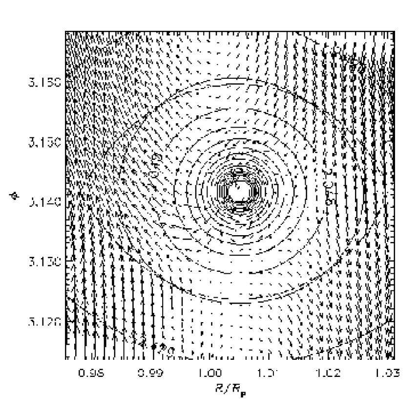
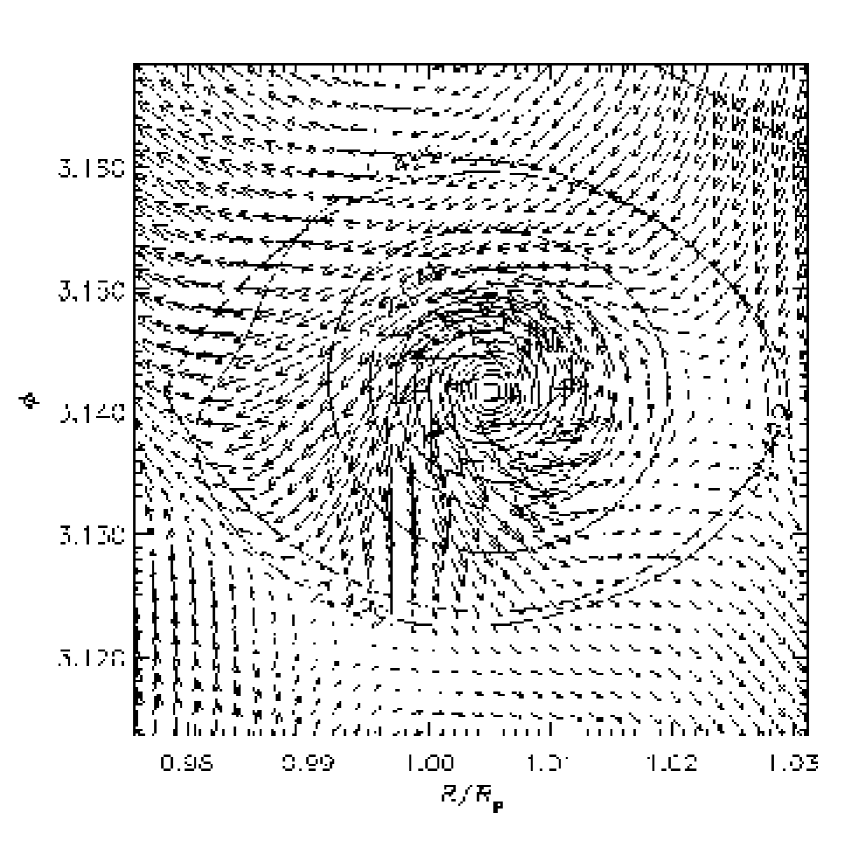
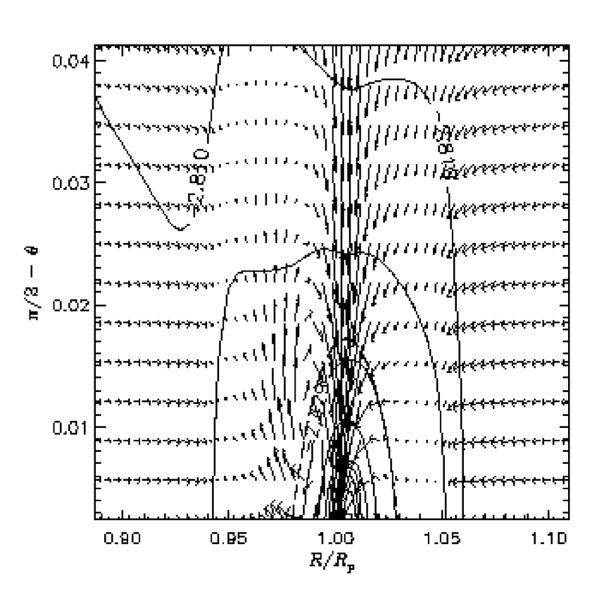
Figure 5: Two-component velocity field on the equatorial plane (top row ) and on the slice $\varphi=\varphi_{\mathrm{p}}$ (middle and bottom rows) for a non-accreting, $20\;M_{\oplus}$ planet (left panels), and an accreting planet of the same mass (right panels) with an accreting sphere radius $\kappa_{\mathrm{ac}}=0.15\,R_{\mathrm{H}}$. Lines of equal $\log{\rho}$ are also drawn. The dashed line represents the Roche lobe of the restricted three-body problem. In the accreting model, the equatorial flow ($\theta=\pi/2$) in the planet’s envelope has a Mach number $\mathcal{M}\lesssim 1.2$ whereas, for the meridional flow, $\mathcal{M}\lesssim 2$. In the non-accreting computation the fluid travels subsonically in both the midplane and the meridional slice ($\mathcal{M}\lesssim 0.2$).

4.2 Gravitational Torques and Orbital Migration

Gravitational torques are believed to be responsible for the migration of protoplanets from their initial formation sites. In this work torques are directly estimated from the gravitational force exerted by each fluid element of the circumstellar disk on the planet. When computing the gravitational force, we consider the density solution on the finest available grid level. This procedure permits to obtain higher accuracy because of the increasing resolution of hierarchy levels.

Since the planet is an extended object, torques acting on each of its portions should be calculated and then added up to give the total torque vector, whose most general expression is

$$\boldsymbol{\mathcal{T}_{\mathrm{D}}} = \int_{M_{\mathrm{D}}}\int_{M_{\mathrm{p}}}(\boldsymbol{R}_{\mathrm{p}}\boldsymbol{+}\boldsymbol{S})$$ (13)

$$\boldsymbol{\times} \frac{G\,dM_{\mathrm{D}}(\boldsymbol{R})\,dM_{\mathrm{p}}(\boldsymbol{S})}{|\boldsymbol{R}-\boldsymbol{R}_{\mathrm{p}}-\boldsymbol{S}|^{3}}\,\boldsymbol{R}\,.$$

Equation (13) explicitly states that circumstellar material can alter both the orbital and rotational spins of a protoplanet. However, here we shall confine our study to variations of the planet’s orbital angular momentum because the evaluation of the rotational spin requires a rigorous treatment of the envelope self-gravity. This is not done here, as stated in § 2 (see eq. [1]). Thereby, we can proceed as if the whole planetary mass were concentrated in its geometrical center $\boldsymbol{R}=\boldsymbol{R}_{\mathrm{p}}$ and integrate the force over the whole disk domain, excluding the volume $\mathcal{V}_{\mathrm{p}}$ occupied by the planetary envelope. Yet, outside of such volume the gravitational potential is always that of a point-mass object (see the behavior of eqs. [4], [6], [7], and [9], for $S>S_{\mathrm{p}}$), therefore equation (13) simplifies and becomes

$$\boldsymbol{\mathcal{T}_{\mathrm{D}}}=\boldsymbol{R}_{\mathrm{p}}\boldsymbol{\times}\int_{\boldsymbol{R}\notin\mathcal{V}_{\mathrm{p}}}\nabla\Phi^{\mathrm{PM}}_{\mathrm{p}}\,\rho(\boldsymbol{R})\,dV(\boldsymbol{R}).$$ (14)

The orbital angular momentum of a protoplanet can be affected only by the $z$-component (that parallel to the polar axis) of the torque vector $\boldsymbol{\mathcal{T}_{\mathrm{D}}}$. To avoid useless distinctions, we indicate this component as $\mathcal{T}_{\mathrm{D}}$. The sign of $\mathcal{T}_{\mathrm{D}}$ determines the gain (positive torques) or loss (negative torques) of orbital spin. Larger spins correspond to more distant orbits. Since torques generally change on time scales on the order of $\sim 50$ revolutions, we work with their final magnitudes. We usually observe a slow decay of $|\mathcal{T}_{\mathrm{D}}|$ with time (see also the end of § 4.3).

Two-dimensional computations reveal that torques exerted by circumplanetary material may amount to a fair fraction of the total torque, unless a suitable smoothing length (usually of the size of the Hill radius) is used in the planet gravitational potential $\Phi_{\mathrm{p}}$. This is caused by the high surface densities reached around the planet and the lack of a vertical torque decay which naturally occurs in three dimensions (see § 5). In fact, in 3D, we observe that torques arising from locations close to the planet do not play such an important role as they do in 2D.

Analyzing the relative strength of torques exercised by different disk portions, it turns out that in the mass range $q\in[2\times 10^{-4},1\times 10^{-3}]$, dominating negative torques arise from distances $S\gtrsim 1.2\,h\,R_{\mathrm{p}}$, where $h$ is the disk aspect ratio. Below $33\;M_{\oplus}$, the largest net contributions are generated by material lying between $S\simeq 0.6\,h\,R_{\mathrm{p}}$ and $S\simeq 2.2\,h\,R_{\mathrm{p}}$. Therefore we can conclude that predominant torques are exerted at distances from the planet comparable with the Hill radius. Not more than 10% of $\mathcal{T}_{\mathrm{D}}$ is built up by matter located within $S\approx 0.6\,h\,R_{\mathrm{p}}$.

Apart from the $20\;M_{\oplus}$ protoplanet, the total torque evaluated in non-accreting models does not deviate considerably from that estimated in accreting ones, independently of the used potential. In fact, simulations based on the potentials $\Phi^{\mathrm{PM}}_{\mathrm{p}}$, $\Phi^{\mathrm{HS}}_{\mathrm{p}}$, and $\Phi^{\mathrm{ST}}_{\mathrm{p}}$ (eqs. [4], [6], and [7], respectively) supply values of $\mathcal{T}_{\mathrm{D}}$ which differ by less than 40%. This circumstance may signify that, whether or not a protoplanet is still accreting matter from its surroundings, this is not generally crucial to the gravitational torques by the circumstellar disk. Thereby, being an exception, the case $M_{\mathrm{p}}=20\;M_{\oplus}$ deserves some comments. For such mass, the torque integrated over the first two grid levels ($S\gtrsim 2.2\,h\,R_{\mathrm{p}}$) yields a positive value for both accreting and non-accreting planets. When adding the contributions from the third and forth level ($0.6\,h\,R_{\mathrm{p}}\lesssim S\lesssim 2.2\,h\,R_{\mathrm{p}}$), the torque experienced by the planet lowers but, while it becomes negative in the accreting case, it still remains positive in the non-accreting counterpart. It is especially matter residing between $1$ and $2\,R_{\mathrm{H}}$ from the planet that builds up the difference. As material in the uppermost grid level ($S\lesssim 0.6\,h\,R_{\mathrm{p}}$) of the non-accreting simulation does not exert any significant torques (some little negative contribution is indeed measured in the accreting model), $\mathcal{T}_{\mathrm{D}}$ keeps the positive sign although, in magnitude, it is eleven times as small as that evaluated in the accreting case. This phenomenon of torque reversal for non-accreting planets with masses of about $20\;M_{\oplus}$ may be related to the very long migration time scales obtained for fully accreting models having masses $M_{\mathrm{p}}\approx 10\,M_{\oplus}$ (see below, and Fig. 6).

Conservation of orbital angular momentum implies that a protoplanet has to adjust its orbital distance from the central star because of external torques exerted by the disk. If the orbit remains circular, the time scale over which this radial drift motion happens is inversely proportional to $\mathcal{T}_{\mathrm{D}}$, according to the formula:

$$\tau_{\mathrm{M}}=\frac{a}{|\dot{a}|}=\frac{M_{\mathrm{p}}\,a^{2}\,\Omega_{\mathrm{p}}}{2\,|\mathcal{T}_{\mathrm{D}}|}.$$ (15)

In equation (15) we indicated with $\Omega_{\mathrm{p}}$ and $a$ the planet’s angular velocity and its distance from the star, respectively. Linear, analytical theories (e.g., Ward, 1997) provide two separate regimes governing the migration of low- (type I) and high-mass (type II) protoplanets. Both migration types predict that the planet moves toward the star. More recent studies by Masset (2001) and Tanaka, Takeuchi, & Ward (2002) have reconsidered the role of co-orbital corotation torques and proved that they can be very effective in opposing Lindblad torques. Hence, they can significantly slow down inward migration. Two-dimensional results presented in Paper II well fit to these predictions. A further reduction of the migration speed is expected from a full 3D treatment of torques, as also derived numerically by Miyoshi et al. (1999) and theoretically predicted by Tanaka, Takeuchi, & Ward (2002).

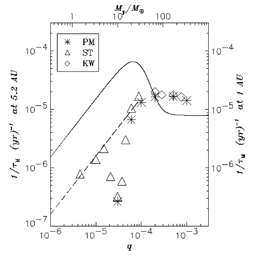
Figure 6: Migration time scale versus the mass ratio $q=M_{\mathrm{p}}/M_{\bigstar}$. Outcomes from simulations carried out with the various forms of gravitational potential are marked with different symbols. At $q=10^{-4}$ and $6\times 10^{-5}$, calculations carried out with the point-mass potential were initiated with a density gap (see § 3.3). To avoid confusion, migration rates obtained from models with $\Phi_{\mathrm{p}}=\Phi_{\mathrm{p}}^{\mathrm{HS}}$ (eq. [6]) are quoted in Table 5. The solid line represents the theoretical prediction by Ward (1997), which does not include corotation torques and 3D effects. Both are indeed accounted for in the analytical model by Tanaka, Takeuchi, & Ward (2002) (dashed line). The parameter $\pi\,a^{2}\,\Sigma_{\mathrm{p}}/M_{\mathrm{D}}$, needed to draw the analytic curves, was retrieved from the initial surface density profile (see § 3.3). The scale on the right vertical axis gives the migration rates of a protoplanet orbiting at $1\;\mbox{{AU}}$ from the primary.

Figure 6 shows our estimates for the migration time scale $\tau_{\mathrm{M}}$ as computed for models having different masses and in which the potential solutions $\Phi^{\mathrm{PM}}_{\mathrm{p}}$, $\Phi^{\mathrm{KW}}_{\mathrm{p}}$, and $\Phi^{\mathrm{ST}}_{\mathrm{p}}$ were adopted. We compare these values with the two analytical theories developed by Ward (1997) (solid line) and Tanaka, Takeuchi, & Ward (2002) (dashed line). The first of them comprises both migration regimes, though accounting only for Lindblad torques. The second theory is limited to type I migration, albeit it treats both Lindblad and corotation torques. Moreover, the first is explicitly two-dimensional whereas the second is applicable in two as well as three dimensions.

As one can see from Figure 6, numerical results are very similar for $M_{\mathrm{p}}\geq 67\;M_{\oplus}$, yielding $\tau_{\mathrm{M}}\approx 5\times 10^{4}\;\mathrm{years}$, whatever of the four gravitational potential is used (see also Table 5). While this time scale is consistent with Ward’s 1997 description if $M_{\mathrm{p}}=67\;M_{\oplus}$, for more massive planets it is nearly two times as short as the theoretical prediction. The depletion of the disk inside the planet’s orbit is probably responsible for part of the discrepancy (see § 4.5), because Ward’s theory assumes a disk with a constant unperturbed surface density. In the type I regime, our numerical experiments with $\Phi_{\mathrm{p}}=\Phi_{\mathrm{p}}^{\mathrm{ST}}$ (eq. [7]) well reproduce the behavior of the analytical curve when $M_{\mathrm{p}}=30$, $20$, $5$, $3.3$, and $1.5\;M_{\oplus}$.

Computations executed with $\Phi_{\mathrm{p}}=\Phi_{\mathrm{p}}^{\mathrm{HS}}$ (eq. [6]) probably underestimate the magnitude of differential torques because of the much weaker gravitational field. Nevertheless, for Jupiter-mass and Earth-mass protoplanets, migration times yielded by these models well compare to those displayed in Figure 6, as proved by the values reported in Table 5.

Table 5: Migration Times obtained with the Homogeneous Sphere Potential.

			$\tau_{\mathrm{M}}\;[\mathrm{years}]$
$M_{\mathrm{p}}/M_{\oplus}$	$q$		Accretion		No Accretion
333	$1.0\times 10^{-3}$		$5.04\times 10^{4}$		$4.80\times 10^{4}$
166	$5.0\times 10^{-4}$		$4.76\times 10^{4}$		$\cdots$
033	$1.0\times 10^{-4}$		$2.10\times 10^{5}$		$2.54\times 10^{5}$
020	$6.0\times 10^{-5}$		$5.74\times 10^{5}$		$\cdots$
010	$3.0\times 10^{-5}$		$5.26\times 10^{5}$		$4.78\times 10^{5}$
005	$1.5\times 10^{-5}$		$6.19\times 10^{5}$		$\cdots$

Note. — Migration rates from accreting and non-accreting models in which $\Phi_{\mathrm{p}}=\Phi_{\mathrm{p}}^{\mathrm{HS}}$ (eq. [6]). Time scales are sensibly different from those indicated in Figure 6 only at $M_{\mathrm{p}}=33$, $20$, and $10\;M_{\oplus}$.

Significant deviations from the linear estimate of Tanaka, Takeuchi, & Ward (2002) are observed in the mass interval $[7,15]\;M_{\oplus}$, where the migration time is longest at $10\;M_{\oplus}$. For this planet $\tau_{\mathrm{M}}$, estimated with Stevenson’s as well as the point-mass potential, is thirty times as long as the theoretical description by Tanaka, Takeuchi, & Ward (2002) predicts. This depends on the strong positive torques arising at $S>2\,h\,R_{\mathrm{p}}$ which are not efficiently contrasted by negative ones generated inside $S\simeq h\,R_{\mathrm{p}}$. However, for this particular planetary mass, we obtain discrepant estimates from computations performed with different resolutions. In fact, the simulation carried out with the grid G2 yields a positive total torque acting on the planet, i.e., it predicts an outward migration, whereas models based on the higher resolution hierarchies G3 and G4 provide a negative total torque. Yet, the absolute value of $\mathcal{T}_{\mathrm{D}}$ evaluated with grid G4 is a seventh of that achieved with grid G3.

Since we believe that gravitational torques are accounted for in a more accurate fashion by hierarchy G3 than by grid G4 because of the arguments in § 4.5, we may rely more on the outcome of the hierarchy G3 (shown Fig. 6) rather than on the other two. We note that such migration time ($\tau_{\mathrm{M}}=3.3\times 10^{6}$ years) is roughly the double of that supplied by the $M_{\mathrm{p}}=10\;M_{\oplus}$, non-accreting model.

We have further inquired into the matter by running a simulation with $M_{\mathrm{p}}=12.5\;M_{\oplus}$ and $\Phi_{\mathrm{p}}=\Phi^{\mathrm{ST}}_{\mathrm{p}}$ (see Table 1). Based on the experience acquired with models executed with grids G3 and G4, we set up the high-resolution hierarchy G5 (see Table 2). This grid is designed to better resolve those regions responsible for the strongest torque contributions in the mass interval $[7,15]\;M_{\oplus}$. As seen in Figure 6, the resulting migration rate follows the trend established by the other assessments in this range of masses.

The interesting property that computed migration time scales are very long for $10\;M_{\oplus}$ planets may be caused by non-linearity effects. We note, in fact, that in numerical simulations the first traces of a trough in the density structure is observed around the same value of $M_{\mathrm{p}}$ and gap formation starts when disk-planet interactions become non-linear. However, this issue needs to be addressed more thoroughly with future computations.

4.3 Mass Accretion

Figure 7: Planet’s accretion rate as function of the normalized planet mass $q$. Different symbols stand for the different forms of gravitational potential $\Phi_{\mathrm{p}}$ adopted in the computations. Apart from those models run with the homogeneous sphere potential $\Phi_{\mathrm{p}}^{\mathrm{HS}}$ (see eq. [6]), mass is removed from a volume, centered on the planet, with radius $\kappa_{\mathrm{ac}}=0.1\,R_{\mathrm{H}}$ (see Table 3 for some details concerning the simulation with $M_{\mathrm{p}}=1.5\;M_{\oplus}$). Models for which $\Phi_{\mathrm{p}}=\Phi_{\mathrm{p}}^{\mathrm{HS}}$ have $\kappa_{\mathrm{ac}}$ equal to $0.2\,R_{\mathrm{H}}$ if $M_{\mathrm{p}}>20\;M_{\oplus}$ and to $0.15\,R_{\mathrm{H}}$ if $M_{\mathrm{p}}=20\;M_{\oplus}$; otherwise $\kappa_{\mathrm{ac}}$ is set to $0.1\,R_{\mathrm{H}}$.

Three-dimensional computations of one Jupiter-mass bodies provide estimates of the mass accretion rate $\dot{M}_{\mathrm{p}}$ on the same order of magnitude as those obtained by two-dimensional ones (see Paper I). Two-dimensional calculations performed by the authors reveal a maximum of the accretion rate, as function of the mass, around $0.5\;M_{\jupiter}$ (see Paper II). Yet, those estimates appear surprisingly high in the very low mass limit. Part of the reasons may lie in the assumed flat geometry which cannot account for the vertical density stratification. The present simulations overcome this restriction, hence they permit to evaluate also the effects due to the disk thickness.

The values of $\dot{M}_{\mathrm{p}}$ is plotted against the planetary mass in Figure 7. As comparison, estimates relative to models with different gravitational potential solutions are shown. The overall behavior of the data points resembles that reported in Paper II, with a peak around $0.3\;M_{\jupiter}$. For $M_{\mathrm{p}}=1\;M_{\jupiter}$ the agreement between two and three-dimensional models is very good and not much discrepancy is seen down to $M_{\mathrm{p}}=20\;M_{\oplus}$, since values are comparable within a factor 3 (see § 4.4). Below this mass, however, the accretion rate rapidly declines, which drop is not observed in 2D outcomes. In fact, one can infer from Figure 7 that the dynamical range of $\dot{M}_{\mathrm{p}}$ stretches for more than two orders of magnitude. By using model results obtained applying the point-mass, Stevenson’s, and Wuchterl’s potential (eqs. [4], [7], and [9], respectively) the following approximate relation can be found:

$$\log\left[\frac{\dot{M}_{\mathrm{p}}}{M_{\oplus}/yr}\right]\simeq b_{0}+b_{1}\,\log{q}\,+b_{2}\,\left(\log{q}\right)^{2},$$ (16)

whose coefficients are $b_{0}=-18.47\pm 0.76$, $b_{1}=-9.25\pm 0.38$, and $b_{2}=-1.266\pm 0.046$. Equation (16) holds as long as the mass ratio $q\in[4.5\times 10^{-6},10^{-3}]$ or, for a one solar-mass star, when $1.5\;M_{\oplus}\leq M_{\mathrm{p}}\leq 1\;M_{\jupiter}$. Such an equation can be applied to scenarios studying the global long-term evolution of young planets.

Calculations in which the homogeneous sphere potential $\Phi^{\mathrm{HS}}_{\mathrm{p}}$ (eq. [6]) is adopted yield accretion rates substantially lower (from $3$ to $15$ times) than those achieved when the other potential forms are employed. This is due to the weak gravitational attraction this potential exerts within the planet’s envelope. As proved by Figure 1, the gravitational field can be $100$ times as small as that established by the other three potential functions for $S\leq S_{\mathrm{p}}$. Also in this circumstance, a relation similar to equation (16) exists for which the coefficients are $b_{0}=-19.42\pm 2.68$, $b_{1}=-9.96\pm 1.41$, and $b_{2}=-1.42\pm 0.18$.

While the accretion rate is fairly stable with time for masses below $30\;M_{\oplus}$, it keeps reducing for higher masses. Between $67\;M_{\oplus}$ and $0.8\;M_{\jupiter}$, $\dot{M}_{\mathrm{p}}$ drops by 10 to 20% during the last $50$ orbits of the simulations. This is an indication of a deepening gap and a depleting disk. As for the dependency upon the accretion volume, from our numerical experiments it is found that doubling the radius $\kappa_{\mathrm{ac}}$, the accretion rate grows at most by 30%. The smaller the planet mass, the less sensitive $\dot{M}_{\mathrm{p}}$ is to the parameter $\kappa_{\mathrm{ac}}$.

4.4 Comparison with 2D Models

Figure 8: Left panel. Migration rates as evaluated in two-dimensional (Paper II) and three-dimensional models (this paper). Right panel. Using the same sources as in the left panel, a comparison of the growth time scales $\tau_{\mathrm{G}}\equiv M_{\mathrm{p}}/\dot{M}_{\mathrm{p}}$, between 2D and 3D outcomes, is shown. Filled triangles, in both panels, indicate results obtained from three-dimensional models in which the planetary gravitational potential is $\Phi_{\mathrm{p}}^{\mathrm{PM}}$, $\Phi_{\mathrm{p}}^{\mathrm{ST}}$, or $\Phi_{\mathrm{p}}^{\mathrm{KW}}$.

In this Section we aim at comparing the migration time scale as well as the planet’s accretion rate obtained in this work with those presented in Paper II. However, while two-dimensional estimates of $\dot{M}_{\mathrm{p}}$ (Fig. 25 in Paper II) are directly comparable to those plotted here in Figure 7, the time scales $\tau_{\mathrm{M}}$ shown in Figure 20 of Paper II are not completely consistent with those in Figure 6. Therefore, they need to be corrected.

This is because in the present study torques are integrated all over the disk domain excluding the planet envelope, i.e., the sphere of radius $S=S_{\mathrm{p}}$. Instead, in Paper II the excluded region has a radius $\approx 0.1\,R_{\mathrm{H}}$ (for details see Paper II, § 5.4). From Table 1 one can see that, above $33\;M_{\oplus}$, the envelope radius $S_{\mathrm{p}}$ can be much larger than a tenth of the Hill radius.

Figure 8 illustrates the migration rate $\tau_{\mathrm{M}}$ (left panel) and the growth time scale $\tau_{\mathrm{G}}\equiv M_{\mathrm{p}}/\dot{M}_{\mathrm{p}}$ (right panel) as computed in the two geometries. Orbital migration estimated by means of 3D simulations is slower than that evaluated in 2D calculations only below $33\;M_{\oplus}$ ($q=10^{-4}$). As for planet’s accretion, the most important difference is the rapid drop, for $M_{\mathrm{p}}<10\;M_{\oplus}$, observed in disks with thickness. The larger values of three-dimensional estimates, measured in the range $10\;M_{\oplus}\lesssim M_{\mathrm{p}}\lesssim 1\;M_{\jupiter}$, are due to the gap which is not so deep as it is in two-dimensional models, hence the average density around the planet is higher. This occurrence can be partly attributed to gravitational potential effects that, as we mentioned in § 4.1, are intensified by the flat geometry approximation.

4.5 Numerical Effects

In Paper II it was found that, upon increasing the smoothing parameter, there is a reduction of the torques’ mismatch, over a region around the planet whose linear size is comparable with the double of the smoothing length. A $33\;M_{\oplus}$ model was run with a point-mass potential without any kind of softening. This is possible because none of the hydrodynamical variables is placed at a cell corner, where the planet dwells. A similar simulation was performed applying a grid dependent smoothing of the type described in Paper II. Resulting migration time scale and mass accretion are not significantly affected by the smoothing choice.

As for the consequences of the circumstellar disk depletion, inside of the planet’s orbit, we ran a Jupiter-mass model in which both inner and outer radial borders were closed. Since more material is available in the disk portion $R<R_{\mathrm{p}}$ (roughly twelve times as much), one should expect larger values for both $\dot{M}_{\mathrm{p}}$ and $\tau_{\mathrm{M}}$. Indeed, accretion is two times as much as that calculated in the model with open inner border. Positive torques arising from the inner disk are also stronger and $\mathcal{T}_{\mathrm{D}}$ is reduced by 50%, i.e., the migration time scale is two times as long.

When simulating a Jupiter-size body embedded in a disk with no initial gap, a density indentation is gradually carved in. In order to skip the gap formation phase, an approximate analytical gap is sometimes imposed in the initial density distribution (see Kley, 1999). We performed three computations adopting this choice. In these cases, a partial shrinking and refilling of the analytical gap is observed. Besides, material drains out of the inner radial border faster than it does in our standard models (no initial gap). Hence, the inner disk depletion is intensified. With respect to standard models, we measure smaller accretion rates and longer migration time scales. Discrepancies in both quantities stay below 20%, after 200 orbits. However, since the model outcomes indicate a tendency to converge as the evolution proceeds, a more appropriate comparison should be made after a long-term evolution.

4.5.1 Grid Resolution

Hardly any hydrodynamic calculation is strictly resolution independent. Thus, for completeness we analyze in this section how our estimates on migration and accretion vary because of different hierarchy resolutions. Two tests are presented for each of the quantities $\dot{M}_{\mathrm{p}}$ and $\mathcal{T}_{\mathrm{D}}$. They are computed with the aid of grid systems G3 and G4 and then results are tested against those calculated with the less resolved hierarchy G2 (see Table 2). In this way we aim at checking finite resolution effects in the radial and azimuthal directions and, separately, those in the meridional direction. In fact, G3 and G2 have the same number of grid points in the vertical direction but $\Delta R[\mathrm{G3}]=0.82\,\Delta R[\mathrm{G2}]$ and $\Delta\varphi[\mathrm{G3}]=0.75\,\Delta\varphi[\mathrm{G2}]$. In the other test case (G4 against G2), $R$ and $\varphi$ gridding is unchanged while the number of latitude grid points is nearly doubled.

Figure 9: Left panel. Comparison of the accretion rate $\dot{M}_{\mathrm{p}}$ as computed on grid systems with different resolutions. Squares indicate that the ratios $\dot{M}_{\mathrm{p}}[\mathrm{G4}]/\dot{M}_{\mathrm{p}}[\mathrm{G2}]$ are drawn, whereas triangles refer to the ratios $\dot{M}_{\mathrm{p}}[\mathrm{G3}]/\dot{M}_{\mathrm{p}}[\mathrm{G2}]$ (see text). Right panel. The same type of comparison for the total torque $\mathcal{T}_{\mathrm{D}}$ experienced by the protoplanet. Squares and triangles have the same meaning as before. At $M_{\mathrm{p}}=10\;M_{\oplus}$, we compare results from models with the homogeneous sphere potential given in equation (6), when available (for this particular mass value, see the discussion in § 4.2).

With regard to the mass accretion rate (Fig. 9, left panel) differences are below 20%. Though the number of grid cells in the accretion sphere is enlarged by a factor either $1.7$ or $2$, no systematic tendency seems to arise from this test. Something different happens to the total torque (right panel). In fact, while the increased resolution in the latitude direction $\theta$ does not play any considerable role, the larger number of grid points in $R$ and $\varphi$ causes a reduction of the total torque magnitude between 20 and 30%. This is not at all unexpected. On one hand circumstellar disk spirals are better captured by a finer gridding in the radial and azimuthal dimensions. Thus, Lindblad torques are accounted for in a more accurate fashion. The Figure proves this to be especially true when the ratio $q$ is small, because of the diminishing wave amplitudes. On the other hand, due to the vertical exponential drop of the density and the lack of temperature stratification, disk layers above the midplane do not contribute very much to $\mathcal{T}_{\mathrm{D}}$. A finer resolution along the vertical dimension cannot sensitively modify the total torque outcome.

5 Discussion

Here we devote some further comments to the differences between accreting and non-accreting protoplanets and then to the effects of the vertical density structure on the gravitational torques acting on embedded objects.

5.1 Pressure Effects in Protoplanetary Envelopes

For the purpose of carrying out a local analysis in the vicinity of accreting and non-accreting protoplanets, we introduce a cylindrical coordinate reference system $\{O^{\prime};l,\psi,z\}$ with its origin $O^{\prime}$ coinciding with the planet position and the $z$-axis perpendicular to the disk midplane. Hence, we will have that $S^{2}=l^{2}+z^{2}$. The longitude angle $\psi$ is counterclockwise increasing, and $\psi=\pi$ points toward the star. Supposing that the flow nearby the planet is stationary, neglecting fluid advection and viscosity, the Navier-Stokes equation for the radial momentum reads:

$$\frac{w^{2}_{\psi}}{l}=\frac{\partial\Phi_{\mathrm{p}}}{\partial l}+\frac{1}{\rho}\,\frac{\partial p}{\partial l},$$ (17)

where $w_{\psi}$ is the azimuthal velocity component around the planet. Excluding the particular situation represented by a homogeneous sphere (eq. [6]), the first term on the right hand side of equation (17) is positive (see Fig. 1). Recalling equation (2), we see that the second term is proportional to the density gradient, which is negative, and therefore it reduces the centrifugal acceleration $w^{2}_{\psi}/l$. In Figure 10 we show some quantities, at $z=0$, averaged over the angle $\psi$, regarding the same simulations addressed in § 4.1.1 ($M_{\mathrm{p}}=20\;M_{\oplus}$ with $\Phi_{\mathrm{p}}=\Phi_{\mathrm{p}}^{\mathrm{ST}}$). From the top left panel one can realize that the mean density is indeed higher in the non-accreting case (solid line) than it is in the accreting case (dashed line), as it was argued in § 4.1.1 from the values listed in Table 4. In order to evaluate how much the pressure gradient affects the left hand side of equation (17) in both cases, we plot the average of such quantity ($\langle w_{\psi}^{2}\rangle/l$) in the top right panel of Figure 10. The centrifugal acceleration is much smaller in the envelope of the non-accreting model (solid line) than it is in that of the accreting one. Such circumstance is a clear indication that the envelope is pressure supported in the first case. The behavior of the averaged velocities $\langle w_{\psi}\rangle$ and $\langle w_{l}\rangle$ is shown in the two bottom panels. As expected in a pressure dominated flow, the magnitude of both velocity components is smaller in the non-accreting model (dashed lines).

Figure 10: Midplane quantities ($z=0$ or $\theta=\pi/2$) azimuthally averaged around the protoplanet for two simulations in which $\Phi_{\mathrm{p}}=\Phi_{\mathrm{p}}^{\mathrm{ST}}$ and $M_{\mathrm{p}}=20\;M_{\oplus}$. The solid line belongs to a non-accreting model, the dashed line to an accreting one. Top-left: mass density. Top-right: centrifugal acceleration. Bottom-left: rotational velocity. Bottom-right: velocity component along the radial distance $l$ (see § 5). All of the four quantities indicate that the envelope is mostly pressure supported in the non-accreting case, whereas it is mainly centrifugally supported in the other.

5.2 Torque Overestimation in 2D Geometry

Gravitational torques exerted by a three-dimensional disk onto a medium- or low-mass protoplanet are weaker than those generated by a two-dimensional disk. Miyoshi et al. (1999) state that the total torque $\mathcal{T}_{\mathrm{D}}$ in 3D is $0.43$ times as small as that in 2D. Something similar was found by Tanaka, Takeuchi, & Ward (2002). Our fully non-linear calculations predict that low-mass protoplanets have a migration rate, at least, an order of magnitude less in disks with thickness than they have in infinitesimally thin disks. One of the main reasons for that relies upon the vertical decay of the density, as one can demonstrate easily with a simplified approach.

Let $t_{z}$ be the $z$-component of the gravitational torque exerted by a column of mass $\Sigma\,l\,dl\,d\psi$, located at distance $l$ from the planet (see § 5.1). The surface density is defined as $\Sigma=\int\rho\,dz$. If $f_{\mathrm{g}}$ is the force exerted by such mass distribution, projected on the equatorial plane, then we can write

$$t_{z}=R_{\mathrm{p}}\,f_{\mathrm{g}}\,\sin{\psi}.$$ (18)

The ratio of $t_{z}[\mathrm{3D}]$ to $t_{z}[\mathrm{2D}]$ is therefore equal to

$$\chi=\frac{f_{g}[\mathrm{3D}]}{f_{g}[\mathrm{2D}]}=\frac{l^{3}}{\Sigma}\int_{-\infty}^{+\infty}\frac{\rho}{(l^{2}+z^{2})^{3/2}}\,dz.$$ (19)

Since $f_{g}[\mathrm{3D}]$ and $f_{g}[\mathrm{2D}]$ are coherent in sign, $\chi$ is also equal to the ratio of $|t_{z}[\mathrm{3D}]|$ to $|t_{z}[\mathrm{2D}]|$. In order to quantify this quantity, we can assume a Gaussian mass density profile with a scale-height $H$, which is appropriate as long as no deep gap has formed. Thus

$$\chi=\frac{l^{3}}{\sqrt{2\pi}\,H}\int_{-\infty}^{+\infty}\frac{\exp{\left(-\frac{z^{2}}{2\,H^{2}}\right)}}{(l^{2}+z^{2})^{3/2}}\,dz.$$ (20)

The ratio $\chi$ as function of $l$ is plotted in Figure 11 and it evidences how a two-dimensional geometry overestimates the magnitude of gravitational torques acting on the protoplanet. In the limit $l^{2}\gg z^{2}$, $\chi$ converges to 1, which proves that only torques arising from locations near to the planet ($l\lesssim H$) are magnified.

Though larger torque magnitudes do not necessarily imply faster migration speeds, they can favor a larger mismatch between negative and positive torques and therefore shorter $\tau_{\mathrm{M}}$.

Figure 11: Ratio of the tree-dimensional to the two-dimensional torque exerted by a column of material lying at a midplane distance $l$ from the protoplanet (see § 5). The upper x-axis is in units of the disk semi-thickness at the planet location: $H=h\,R_{\mathrm{p}}$.

6 Conclusions

On the background of the numerical computations of disk-planet interaction presented in Paper I and II, in this paper we combine the full 3D geometry of a circumstellar disk with a nested-grid technique in order to investigate in detail flow dynamics, orbital decay, and mass accretion of protoplanets in the mass range $[1.5\;M_{\oplus},1\;M_{\jupiter}]$. Besides, we overcome the point-mass assumption by employing analytic expressions of the gravitational potential derived from simple theoretical models of protoplanetary envelopes. Each of them applies to distinct physical situations: when the envelope mass is negligible with respect to the core mass; when the envelope is homogeneous and much more massive than the core; when the envelope is fully radiative, and finally when it is fully convective.

Through a series of 51 simulations, we inspect the evolution and differences of protoplanets represented by the aforementioned gravitational potentials. We analyze the behavior of both accreting and non-accreting objects. Furthermore, we evaluate physical and numerical effects due to our standard set-up of the models. The computations clearly show that to accurately determine the early physical evolution of planets three-dimensional effects have to be taken into account.

The main results of our studies can be summarized as:

1. Above the disk midplane the flow is nearly laminar only far away from the planet. The region of influence of the planet extends well outside the Hill sphere and its boundaries are marked by vertical shock fronts. Past the shock, matter is deflected upward and then downward. In some cases, a closed recirculation is also observed. In the disk midplane, spiral waves around the planet are not as strong and tight as they appear in two dimensions because of wave deflection in the vertical direction.

2. In the mass range of their applicability, Stevenson’s and Wuchterl’s gravitational potentials produce flow structures, close to the planet, similar to those determined by a smoothed point-mass potential. Migration times and accretion rates are alike. In contrast models with the (unrealistic) potential of a homogeneous sphere yield different dynamics though, as for $\tau_{\mathrm{M}}$ and $\dot{M}_{\mathrm{p}}$, not much difference is observed for Jupiter and Earth-size bodies.

3. Since the numerical accretion procedure might be considered somewhat arbitrary, we ran several models in which the protoplanet does not accrete at all. Non-accreting models behave differently from accreting ones in a volume whose size is roughly comparable with the Hill sphere. Within this region matter is pressure supported and thus a spherical envelope builds up. Except for the case $M_{\mathrm{p}}=20\;M_{\oplus}$, the total torque $\mathcal{T}_{\mathrm{D}}$ exerted by the disk is on the same order of magnitude as that measured in accreting models.

4. According to Ward’s theory (Ward, 1997), the migration speed settles to a constant value when the planet-to-star mass ratio $q\gtrsim 4\times 10^{-4}$. Our numerical results give a similar trend at a slightly different magnitude though. Most of these simulations predict an inward migration except the one where a $20\;M_{\oplus}$, non-accreting, protoplanet is involved. In the mass range $[7\;M_{\oplus},15\;M_{\oplus}]$ migration speeds can be 30 times as slow as those predicted by Tanaka, Takeuchi, & Ward (2002) although, outside of this range, the agreement between our computational data and the type I migration by the same authors is remarkably good. We suspect that this surprising outcome may be caused by the onset of non-linear effects appearing around ten Earth’s masses, which conspire to give such long migration time scales. If correct, this much slower inward motion may help to solve the problem of the too rapid drift of planets toward their host stars.

5. In agreement with studies on planet formation (Bodenheimer & Pollack, 1986; Tajima & Nakagawa, 1997), the growth time scale shortens as the protoplanet’s mass increases. The minimum is found at $M_{\mathrm{p}}=20\;M_{\oplus}$. Albeit the feeding process slows down as soon as angular momentum transferred by the planet to the surrounding material is large enough to dig a density gap. Then, at $M_{\mathrm{p}}\approx 1\;M_{\jupiter}$, the accretion rate greatly reduces and the growth time scale becomes consistently very long. We present an analytical formula for the growth rate which may be useful for global studies in planet formation.

6. As long as migration and mass accretion are considered, two-dimensional computations still yields reliable results when the mass ratio $q\gtrsim 10^{-4}$ ($M_{\mathrm{p}}\gtrsim 30\;M_{\oplus}$ if $M_{\bigstar}=1\;M_{\odot}$). In practice, 2D geometry is applicable whenever the Hill radius $R_{\mathrm{H}}$ exceeds the 60% of the local pressure scale-height of the disk $H$. But for smaller masses three-dimensional calculations have to be considered.

The three-dimensional calculations presented here achieve a new level of accuracy by using a sophisticated nested-grid technique. This numerical feature allows a global and local resolution not obtained hitherto. However, similar to all of the previous calculations, the models presented here have one principal limitation: the lack of an appropriate energy equation. Because of this, we could not couple the thermal and the hydrodynamical evolution of the system. If one wishes to do that in three dimensions, the energy equation has to include radiation and convective transfer. Yet, only with massive parallel computations one can hope to pursue this goal. Thereupon, the direction of future developments and improvements is already marked.

Appendix A Interpolation Formulas for the Fine-coarse Grid Interaction

The aim of this appendix is to furnish some algorithms useful for updating the values of scalars and momenta on a coarse grid with those computed on the hosted (finer) grid, in spherical polar coordinates.

For the purpose, we indicate with $\rho^{\mathrm{C}}$ the mass density to be interpolated on the coarse level. The interpolating values, on the finer subgrid level, are indicated simply as $\rho(i,j,k)$. For the density average, the $i$-index varies between $i$ and $i+1$ and so do the other two indexes.

Accordingly, $U^{\mathrm{C}}_{R}$, $U^{\mathrm{C}}_{\theta}$ and $U^{\mathrm{C}}_{\varphi}$ are the coarse linear, meridional and azimuthal angular momentum. The finer values from which they are reset will be denoted as $U_{R}(i,j,k)$, $U_{\theta}(i,j,k)$, and $U_{\varphi}(i,j,k)$, respectively. For the average of the radial vector component, the $i$-index varies between $i-1$ and $i+1$, while the other two indexes vary between $j$ ($k$) and $j+1$ ($k+1$). This is related to the locations where velocity components are defined on the mesh. In case of the meridional angular momentum, the $j$-index ranges from $j-1$ to $j+1$, while the others are $i$ ($k$) and $i+1$ ($k+1$). For the azimuthal angular momentum, it is the $k$-index to extend over the wider range.

The finer grid coordinates are $(R_{i},\theta_{j},\varphi_{k})$, and the grid spacing is $(\Delta R,\Delta\theta,\Delta\varphi)$ (see Fig. 12), which is constant. Since the grid has a staggered structure, scalars are volume-centered, i.e., $\rho(i,j,k)$ lies at $(R_{i}+\Delta R/2,\theta_{j}+\Delta\theta/2,\varphi_{k}+\Delta\varphi/2)$, while $\rho^{\mathrm{C}}$ resides at $(R_{i}+\Delta R,\theta_{j}+\Delta\theta,\varphi_{k}+\Delta\varphi)$, because the linear resolution doubles from a grid to the hosted one. Instead, vector components are centered each on a different face of the volume element. For example, the radial component $U_{R}(i,j,k)$ is located at $(R_{i},\theta_{j}+\Delta\theta/2,\varphi_{k}+\Delta\varphi/2)$, whereas the coarse radial momentum $U^{\mathrm{C}}_{R}$ is defined at $(R_{i},\theta_{j}+\Delta\theta,\varphi_{k}+\Delta\varphi)$. The locations of the other components follow by similarity.

The interpolation is basically a volume-weighted average. Eight volumes are necessary to carry out a scalar interpolation. Momentum interpolations require that twelve spherical sectors must be employed. Yet, since the metric in a spherical polar topology is independent of the azimuthal angle $\varphi$, some of them actually coincide. In order to distinguish among the four volume sets, we introduce the notations $V^{(\rho)}$, $V^{(R)}$, $V^{(\theta)}$ and $V^{(\varphi)}$, according to the quantity to average ($\rho^{\mathrm{C}}$, $U^{\mathrm{C}}_{R}$, $U^{\mathrm{C}}_{\theta}$, and $U^{\mathrm{C}}_{\varphi}$). These four sets differ because of the space metric and the staggered mesh.

Once the correct elements have been identified, the coarse mass density can be replaced by

$$\rho^{\mathrm{C}}=\frac{\sum_{ijk}\rho(i,j,k)\,V^{(\rho)}(i,j)}{2\,\sum_{ij}V^{(\rho)}(i,j)}.$$ (A1)

In fact, sectors $V^{(\rho)}$ are $\varphi$-independent, thus only four volumes enter this average. In a similar fashion, corrected momenta can be written, in a concise form, as

$$U_{\Xi}^{\mathrm{C}}=\frac{\sum_{ijk}U_{\Xi}(i,j,k)\,V^{(\Xi)}(i,j,k)}{\sum_{ijk}V^{(\Xi)}(i,j,k)},$$ (A2)

where $\Xi=R$, $\theta$, and $\varphi$. For computational purposes, a volume element is preferentially cast into the form

$$V=\left(\Delta R^{3}/3\right)\,\left(-\Delta\cos{\theta}\right)\,\left(\Delta\varphi\right).$$ (A3)

The four sectors $V^{(\rho)}$ required in equation (A1) are the following

$$V^{(\rho)}(i,j) = \frac{1}{3}\left(R_{i+1}^{3}-R_{i}^{3}\right)\,\left[\cos{(\theta_{j})}-\cos{(\theta_{j+1})}\right]\,\Delta\varphi$$

$$V^{(\rho)}(i+1,j) = \frac{1}{3}\left[(R_{i+1}+\Delta R)^{3}-R_{i+1}^{3}\right]\,\left[\cos{(\theta_{j})}-\cos{(\theta_{j+1})}\right]\,\Delta\varphi$$

$$V^{(\rho)}(i,j+1) = \frac{1}{3}\left(R_{i+1}^{3}-R_{i}^{3}\right)\,\left[\cos{(\theta_{j+1})}-\cos{(\theta_{j+1}+\Delta\theta)}\right]\,\Delta\varphi$$ (A4)

$$V^{(\rho)}(i+1,j+1) = \frac{1}{3}\left[(R_{i+1}+\Delta R)^{3}-R_{i+1}^{3}\right]$$

$$\left[\cos{(\theta_{j+1})}-\cos{(\theta_{j+1}+\Delta\theta)}\right]\,\Delta\varphi.$$

Also for the radial and meridional directions, the denominator of equation (A2) reduces to $2\,\sum_{ij}V^{(\Xi)}(i,j)$, though the summation includes six terms, this time. Therefore, the set of volume elements necessary for the interpolation of the radial momentum $U^{\mathrm{C}}_{R}$ is:

$$V^{(R)}(i-1,j) = \frac{1}{3}\left[\frac{1}{8}\,(R_{i-1}+R_{i})^{3}-R_{i-1}^{3}\right]$$

$$\left[\cos{(\theta_{j})}-\cos{(\theta_{j+1})}\right]\,\Delta\varphi$$

$$V^{(R)}(i,j) = \frac{1}{24}\left[(R_{i}+R_{i+1})^{3}-(R_{i-1}+R_{i})^{3}\right]$$

$$\left[\cos{(\theta_{j})}-\cos{(\theta_{j+1})}\right]\,\Delta\varphi$$

$$V^{(R)}(i+1,j) = \frac{1}{3}\left[R_{i+1}^{3}-\frac{1}{8}\,(R_{i}+R_{i+1})^{3}\right]$$ (A5)

$$\left[\cos{(\theta_{j})}-\cos{(\theta_{j+1})}\right]\,\Delta\varphi$$

$$V^{(R)}(i-1,j+1) = \frac{1}{3}\left[\frac{1}{8}\,(R_{i-1}+R_{i})^{3}-R_{i-1}^{3}\right]$$

$$\left[\cos{(\theta_{j+1})}-\cos{(\theta_{j+1}+\Delta\theta)}\right]\,\Delta\varphi$$

$$V^{(R)}(i,j+1) = \frac{1}{24}\left[(R_{i}+R_{i+1})^{3}-(R_{i-1}+R_{i})^{3}\right]$$

$$\left[\cos{(\theta_{j+1})}-\cos{(\theta_{j+1}+\Delta\theta)}\right]\,\Delta\varphi$$

$$V^{(R)}(i+1,j+1) = \frac{1}{3}\left[R_{i+1}^{3}-\frac{1}{8}\,(R_{i}+R_{i+1})^{3}\right]$$

$$\left[\cos{(\theta_{j+1})}-\cos{(\theta_{j+1}+\Delta\theta)}\right]\,\Delta\varphi.$$

The group of elements involved in the updating process of the meridional angular momentum $U^{\mathrm{C}}_{\theta}$ is:

$$V^{(\theta)}(i,j-1) = \frac{1}{3}\left(R_{i+1}^{3}-R_{i}^{3}\right)\,\left\{\cos{(\theta_{j-1})}-\cos{[(\theta_{j-1}+\theta_{j})/2]}\right\}\,\Delta\varphi$$

$$V^{(\theta)}(i,j) = \frac{1}{3}\left(R_{i+1}^{3}-R_{i}^{3}\right)$$

$$\left\{\cos{[(\theta_{j-1}+\theta_{j})/2]}-\cos{[(\theta_{j}+\theta_{j+1})/2]}\right\}\,\Delta\varphi$$

$$V^{(\theta)}(i,j+1) = \frac{1}{3}\left(R_{i+1}^{3}-R_{i}^{3}\right)\,\left\{\cos{[(\theta_{j}+\theta_{j+1})/2]}-\cos{(\theta_{j+1})}\right\}\,\Delta\varphi$$

$$V^{(\theta)}(i+1,j-1) = \frac{1}{3}\left[(R_{i+1}+\Delta R)^{3}-R_{i+1}^{3}\right]$$

$$\left\{\cos{(\theta_{j-1})}-\cos{[(\theta_{j-1}+\theta_{j})/2]}\right\}\,\Delta\varphi$$

$$V^{(\theta)}(i+1,j) = \frac{1}{3}\left[(R_{i+1}+\Delta R)^{3}-R_{i+1}^{3}\right]$$

$$\left\{\cos{[(\theta_{j-1}+\theta_{j})/2]}-\cos{[(\theta_{j}+\theta_{j+1})/2]}\right\}\,\Delta\varphi$$

$$V^{(\theta)}(i+1,j+1) = \frac{1}{3}\left[(R_{i+1}+\Delta R)^{3}-R_{i+1}^{3}\right]$$

$$\left\{\cos{[(\theta_{j}+\theta_{j+1})/2]}-\cos{(\theta_{j+1})}\right\}\,\Delta\varphi.$$

In order to perform the interpolation of the azimuthal angular momentum $U^{\mathrm{C}}_{\varphi}$, the following set of volume elements is required:

$$V^{(\varphi)}(i,j,k-1) = \frac{1}{3}\left(R_{i+1}^{3}-R_{i}^{3}\right)\,\left[\cos{(\theta_{j})}-\cos{(\theta_{j+1})}\right]\,\Delta\varphi/2$$

$$V^{(\varphi)}(i+1,j,k-1) = \frac{1}{3}\left[(R_{i+1}+\Delta R)^{3}-R_{i+1}^{3}\right]$$

$$\left[\cos{(\theta_{j})}-\cos{(\theta_{j+1})}\right]\,\Delta\varphi/2$$

$$V^{(\varphi)}(i,j+1,k-1) = \frac{1}{3}\left(R_{i+1}^{3}-R_{i}^{3}\right)$$

$$\left[\cos{(\theta_{j+1})}-\cos{(\theta_{j+1}+\Delta\theta)}\right]\,\Delta\varphi/2$$

$$V^{(\varphi)}(i+1,j+1,k-1) = \frac{1}{3}\left[(R_{i+1}+\Delta R)^{3}-R_{i+1}^{3}\right]$$

$$\left[\cos{(\theta_{j+1})}-\cos{(\theta_{j+1}+\Delta\theta)}\right]\,\Delta\varphi/2$$

$$V^{(\varphi)}(i,j,k) = 2\,V^{(\varphi)}(i,j,k-1)$$ (A7)

$$V^{(\varphi)}(i,j+1,k) = 2\,V^{(\varphi)}(i,j+1,k-1)$$

$$V^{(\varphi)}(i+1,j,k) = 2\,V^{(\varphi)}(i+1,j,k-1)$$

$$V^{(\varphi)}(i+1,j+1,k) = 2\,V^{(\varphi)}(i+1,j+1,k-1)$$

$$V^{(\varphi)}(i,j,k+1) = V^{(\varphi)}(i,j,k-1)$$

$$V^{(\varphi)}(i,j+1,k+1) = V^{(\varphi)}(i,j+1,k-1)$$

$$V^{(\varphi)}(i+1,j,k+1) = V^{(\varphi)}(i+1,j,k-1)$$

$$V^{(\varphi)}(i+1,j+1,k+1) = V^{(\varphi)}(i+1,j+1,k-1).$$

Equations A7 imply that the denominator of equation (A2) is also equivalent to $2\,\sum_{ij}V^{(\varphi)}(i,j,k)$.

Velocities are retrieved from momenta and density. Fine-coarse interaction also involves the correction of momentum flux components across the boundaries between two neighboring grids. This is accomplished via time and surface-weighted means (for details, see Paper II).

Figure 12: Sketch of a spherical sector composed of two coarse grid cells (thick lines) and the set of nested cells (thin lines). The discretized spherical coordinates $(R_{i},\theta_{j},\varphi_{k})$ are relative to the fine grid, and so is the resolution $(\Delta R,\Delta\theta,\Delta\varphi)$. Scalars are cell-centered on each grid level, whereas vector components are face-centered, each on a different face of the volume element.

References

- Agnor & Ward (2002) Agnor, C. B., & Ward, W. R. 2002, ApJ, 567, 579
- Bodenheimer & Pollack (1986) Bodenheimer, P., & Pollack, J. B. 1986, Icarus, 67, 391
- D’Angelo, Henning, & Kley (2002) D’Angelo, G., Henning, Th., & Kley, W. 2002, A&A, 385, 647 (Paper II)
- D’Angelo, Kley, & Henning (2002) D’Angelo, G., Kley, W., & Henning, Th. 2002, to appear in ASP Conf. Ser., Scientific Frontiers in Research on Extrasolar Planets, ed. D. Deming (San Francisco: ASP)
- Goldreich & Tremaine (1980) Goldreich, P., & Tremaine, S. 1980, ApJ, 241, 425
- Kley (1999) Kley W. 1999, MNRAS, 303, 696
- Kley, D’Angelo, & Henning (2001) Kley, W., D’Angelo, G., & Henning, Th. 2001, ApJ, 547, 457 (Paper I)
- Lubow (1981) Lubow, S. H. 1981, ApJ, 245, 274
- Lubow & Pringle (1993) Lubow, S. H., & Pringle, J. E. 1993, ApJ, 409, 360
- Lubow, Seibert, & Artymowicz (1999) Lubow, S. H., Seibert, M., & Artymowicz, P. 1999, ApJ, 526, 1001
- Lynden-Bell & Pringle (1974) Lynden-Bell, D., & Pringle, J. E. 1974, MNRAS, 168, 603
- Makita, Miyawaki, & Matsuda (2000) Makita, M., Miyawaki, K., Matsuda, T. 2000, MNRAS, 316, 906
- Masset (2001) Masset, F. 2001, ApJ, 558, 453
- Masset (2002) Masset, F. 2002, A&A, 387, 605
- Mihalas & Mihalas (1999) Mihalas, D., & Mihalas B. 1999, Foundations of Radiation Hydrodynamics (2d ed.; New York: Dover)
- Miyoshi et al. (1999) Miyoshi, K., Takeuchi, T., Tanaka, H., & Ida, S. 1999, ApJ, 516, 451
- Nelson et al. (2000) Nelson, R., Papaloizou, J. C. B., Masset, F., & Kley, W. 2000, MNRAS, 318, 18
- Ogilvie & Lubow (1999) Ogilvie, G. I., Lubow, S. H. 1999, ApJ, 515, 767
- Papaloizou & Lin (1984) Papaloizou, J. C. B., & Lin, D. N. C. 1984, ApJ, 285, 818
- Papaloizou, Nelson, & Masset (2001) Papaloizou, J. C. B., Nelson, R., & Masset, F. 2001, A&A, 366, 263
- Stevenson (1982) Stevenson, D. J. 1982, Planet. Space Sci., 30, 755
- Tajima & Nakagawa (1997) Tajima, N., & Nakagawa, Y. 1997, Icarus, 126, 282
- Tanaka, Takeuchi, & Ward (2002) Tanaka, H., Takeuchi, T., & Ward, W. 2002, ApJ, 565, 1257
- Tanigawa & Watanabe (2002) Tanigawa, T., & Watanabe, S. 2002, ApJ, preprint doi: 10.1086/343069
- Ward (1986) Ward, W. R. 1986, Icarus, 67, 164
- Ward (1997) Ward, W. R. 1997, Icarus, 126, 261
- Wuchterl (1991) Wuchterl, G. 1991, Icarus, 91, 39
- Wuchterl (1993) Wuchterl, G. 1993, Icarus, 106, 323
- Ziegler & Yorke (1997) Ziegler, U., & Yorke, H.W. 1997, Comput. Phys. Commun., 101, 54
- Ziegler (1998) Ziegler, U. 1998, Comput. Phys. Commun., 109, 111