Principal Power of the CMB

Abstract

We study the physical limitations placed on CMB temperature and polarization measurements of the initial power spectrum by geometric projection, acoustic physics, gravitational lensing and the joint fitting of cosmological parameters. Detailed information on the spectrum is greatly assisted by polarization information and localized to the acoustic regime $k=0.02-0.2$ Mpc^-1 with a fundamental resolution of $\Delta k/k>0.05$. From this study we construct principal component based statistics, which are orthogonal to cosmological parameters including the initial amplitude and tilt of the spectrum, that best probe deviations from scale-free initial conditions. These statistics resemble Fourier modes confined to the acoustic regime and ultimately can yield $\sim 50$ independent measurements of the power spectrum features to percent level precision. They are straightforwardly related to more traditional parameterizations such as the the running of the tilt and in the future can provide many statistically independent measurements of it for consistency checks. Though we mainly consider physical limitations on the measurements, these techniques can be readily adapted to include instrumental limitations or other sources of power spectrum information.

I Introduction

High precision cosmic microwave background (CMB) temperature anisotropy measurements from WMAP have ushered in a new era in the determination of the initial conditions for structure formation and their implications for the physics of the early universe Peietal03 . Hints of deviations from power law initial conditions from WMAP in the form of marginally significant coherent glitches over several multipoles and running of the tilt can be tested by the Planck satellite Planck and definitively measured with a high precision CMB polarization experiment such as the envisaged Inflation Probe CMBPol CMBPol .

Significant deviations would imply that the initial power spectrum is not scale free and hence traditional descriptions such as a constant running of the tilt, motivated by the small deviations expected from slow-roll inflation (e.g. MukFelBra92 ), can lead to misinterpretation and biases in parameter determination.

A large body of work already exists on more general approaches. They are typically based on flat bandpowers, discrete sampling with interpolation for continuity or smoothness, wavelet expansions or more generally some predetermined set of windows on, or effective regularization of, the initial power spectrum MukWan03 ; MilNicGenWas02 ; TegZal02 ; BriLewWelEfs03 .

In this paper, we study the fundamental physical limitations placed on the measurement of the initial power spectrum by geometric projection, acoustic physics, gravitational lensing, and the joint fitting of cosmological parameters. We then use this study to develop complementary techniques that are optimized with respect to the physics of the CMB rather than prior assumptions about the form of the initial power spectrum.

The outline of this paper is as follows. In §II, we study the processes that transfer fluctuations from the initial curvature perturbation to the observed temperature and polarization fields and quantify the limitations imposed by acoustic physics and geometric projection. In §III, we introduce a discrete parameterization of the initial spectrum that is matched to the further limitations imposed by gravitational lensing. In §IV, we employ Fisher matrix techniques to study the effect of joint estimation of the initial spectrum and cosmological parameters. In §V, we construct modes which best constrain from scale-free initial conditions out of its principal components. We conclude in §VI.

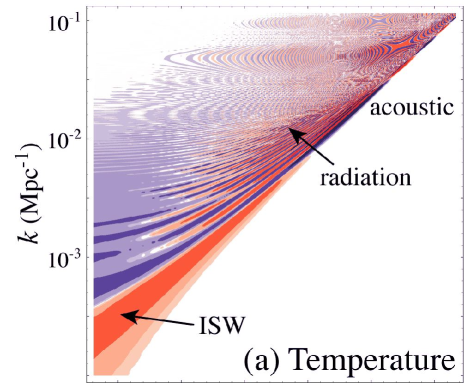
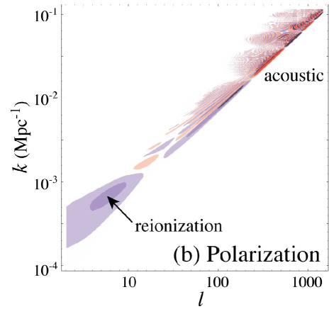
Figure 1: Transfer functions in temperature and polarization Contours are spaced by factors of 4 with blue (red) denoting fluctuations with the same (opposite) sign as $\zeta$. Note the projection ridge along the diagonal, the out-of-phase temperature and polarization acoustic oscillations along the ridge beginning with the Sachs-Wolfe (SW) effect for the temperature, the reionization bump for the polarization, and the potential decay terms from the dark energy (ISW) and radiation for the temperature. The polarization transfer is cleaner than and complementary to the temperature transfer.

II Transfer Functions and Projection

Acoustic and gravitational physics generate CMB temperature fluctuations $\Theta=\Delta T({\hat{\bf n}})/T$ and polarization fluctuations $E({\hat{\bf n}})$ ZalSel97 in the angular direction ${\hat{\bf n}}$ from an initial spatial curvature fluctuation $\zeta({\bf x})$, which we will specify in the comoving gauge. The observable angular power spectra are defined by the two point function of their multipole moments

$$\langle X_{\ell m}^{*}X^{\prime}_{\ell^{\prime}m^{\prime}}\rangle=\delta_{\ell\ell^{\prime}}\delta_{mm^{\prime}}C_{\ell}^{XX^{\prime}}\,,$$ (1)

where $X,X^{\prime}\in\Theta,E$ and consequently are related to the initial curvature power spectrum

$$\langle\zeta^{*}({\bf k})\zeta({\bf k}^{\prime})\rangle=(2\pi)^{3}\delta({\bf k}-{\bf k}^{\prime}){2\pi^{2}\over k^{3}}{\Delta^{2}_{\zeta}}(k)\,.$$ (2)

For slow-roll inflation the initial spectrum is given by (e.g. see MukFelBra92 )

$$\Delta_{\zeta}^{2}(k)={G\over\pi\epsilon}H^{2}_{i}\,,$$ (3)

where $H_{i}$ is the Hubble parameter, $\epsilon=3(1+w_{i})/2$, and $w_{i}$ is the equation of state, all evaluated when the $k$-mode exited the horizon during inflation. To the extent that $H_{i}$ and $w_{i}$ are constant, the spectrum is scale invariant; to the extent that the evolution is small across observable scales, the spectrum is a scale-free power law.

The mappings between the two sets of power spectra are specified by transfer functions

$${\ell(\ell+1)C_{\ell}^{XX^{\prime}}\over 2\pi}=\int{d\ln k}\,T^{X}_{\ell}(k)T^{X^{\prime}}_{\ell}(k)\,\Delta_{\zeta}^{2}(k)\,.$$ (4)

Note that unlike the familiar transfer function of the matter power spectrum, the CMB transfer functions are inherently two-dimensional since they convert spatial fluctuations to angular fluctuations HuSug95b .

These transfer functions are obtained by numerically solving the linearized Einstein-Boltzmann equations. The publically available CMBFast SelZal96 and CAMB LewChaLas00 integral codes do return these functions in principle. However they implicitly assume that the initial conditions are smooth so that the observable power spectra can be rapidly calculated by interpolation in $\ell$ and $k$. This interpolation can cause problems if the initial power spectrum contains features that are comparable to the gridding, e.g. typically $\Delta\ell=50$. Traditional Boltzmann hierarchy codes WilSil81 ; BonEfs84 ; WhiSco96 on the other hand solve the equations for every $\ell<\ell_{\rm max}$ but typically sample sparsely in the computationally costly $k$-modes and so require explicit smoothing in $\ell$ HuScoSugWhi95 .

We have instead developed an independent, fast version of a Boltzmann hierarchy code whose speed without smoothing is comparable to the public codes with an evaluation at every $\ell$. Specifically the code solves the linearized equations HuSelWhiZal98 and the multilevel-atom calibrated 2-level hydrogen and helium recombination equations SeaSasSco99 in the comoving gauge out to $\ell_{\rm max}=6000$ with absorptive boundary conditions. We have checked that the agreement with CMBFast v4.3 with RECFast for smooth initial conditions is typically at the few $10^{-3}$ level and comparable to the numerical error in CMBFast SelSugWhiZal03 .

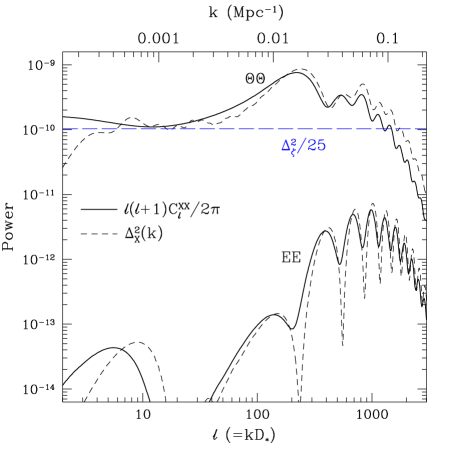
Figure 2: CMB angular and spatial power spectra for the fiducial cosmology and spectrum $\Delta_{\zeta}^{2}=(5.07\times 10^{-5})^{2}$. The spatial power spectra $\Delta^{2}_{X}(k)$ are plotted with $k=\ell/D_{*}$. The low $k$ cutoff is due to $\ell_{\rm min}=2$ and corresponds to superhorizon scale modes. Asymmetry in the projection leads to $\ell<kD_{*}$ power that is much more pronounced in the temperature than the polarization.

For this work, we oversample the transfer functions with 3750 logarithmically spaced $k$-modes from $k=10^{-4.35}-10^{-1.35}$ Mpc^-1 ($\delta k/k=1.8\times 10^{-3}$) and 2500 $k$-modes from $10^{-1.35}-10^{-0.35}$ Mpc^-1 ($\delta k/k=0.9\times 10^{-3}$). Figure 1 shows the transfer functions for the fiducial flat cosmology with dark energy density $\Omega_{\rm DE}=0.72$, dark energy equation of state $w=-1$, matter density $\Omega_{m}h^{2}=0.145$, baryon density $\Omega_{b}h^{2}=0.024$ and reionization optical depth $\tau=0.17$.

The most notable feature of the transfer functions is the main projection ridge along the diagonal at $kD_{*}=\ell$, where the angular diameter distance to recombination $D_{*}=13.8$Gpc in the fiducial model. It is instructive to consider first the simple Sachs-Wolfe (SW) SacWol67 limit of purely gravitational effects in a flat universe. Here the temperature fluctuation is a projection of $1/3$ of the Newtonian gravitational potential or equivalently $1/5$ of the comoving curvature,

$$\Theta_{\ell m} = \int d{\hat{\bf n}}Y_{\ell m}^{*}({\hat{\bf n}})\Theta({\hat{\bf n}})$$

$$= \int d{\hat{\bf n}}Y_{\ell m}^{*}({\hat{\bf n}}){1\over 5}\zeta({\bf x}=D_{*}{\hat{\bf n}})$$

$$= {4\over 5}\pi\int{d^{3}k\over(2\pi)^{3}}i^{\ell}j_{\ell}(kD_{*})Y_{\ell m}^{*}(\hat{\bf k})\zeta({\bf k})\,,$$

$$E_{\ell m} = 0\,.$$ (5)

Terefore comparing Eqn. (1) (2) and (4), we obtain

$$T_{\ell}^{\Theta}(k) = {\sqrt{2\ell(\ell+1)}\over 5}j_{\ell}(kD_{*})\,,$$

$$T_{\ell}^{E}(k) = 0\,.$$ (6)

By further assuming a fiducial model with a scale-invariant initial power spectrum

$$\Delta_{\zeta}^{2}(k)\big{|}_{\rm fid}=\delta_{\zeta}^{2}=(5.07\times 10^{-5})^{2}\,,$$ (7)

we can evaluate the integral over $\ln k$ to obtain

$${\ell(\ell+1)\over 2\pi}C_{\ell}^{\Theta\Theta} = {\Delta_{\zeta}^{2}\over 25}\,,$$

$${\ell(\ell+1)\over 2\pi}C_{\ell}^{EE} = 0\,.$$ (8)

The sums over $\ln\ell$ yield the spatial power spectra

$$\Delta_{\Theta}^{2}(k) = \sum_{\ell=2}^{\ell_{\rm max}}{1\over\ell}T_{\ell}^{\Theta}(k)T_{\ell}^{\Theta}(k)\Delta_{\zeta}^{2}\approx{\Delta_{\zeta}^{2}\over 25}\,,\quad(\ell\gg 1)\,,$$

$$\Delta_{E}^{2}(k) = \sum_{\ell=2}^{\ell_{\rm max}}{1\over\ell}T_{\ell}^{E}(k)T_{\ell}^{E}(k)\Delta_{\zeta}^{2}=0\,,$$ (9)

which quantifies the contribution per log interval to the field variance $\langle X({\hat{\bf n}})X({\hat{\bf n}})\rangle$ BonEfs87 . Thus geometric projection represents a power conserving mapping described by the spherical Bessel function $j_{\ell}(kD_{*})$. Under the SW approximation the transfer function of Fig. 1 would appear as a diagonal band that narrowed with increasing $k$.

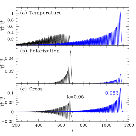
Figure 3: Angular spectrum of an individual $k$ mode for a trough $k_{m\approx 5/2}=0.05$ Mpc^-1 and a peak $k_{m\approx 4}=0.082$ Mpc^-1. At acoustic troughs, the temperature perturbations are dominated by the Doppler effect which is smeared out in angle by the projection; here the polarization is at its maximum and yields a sharp projection of power.

The actual transfer functions differ from the SW approximation in interesting ways. Figure 2 compares the $\ell$-space and $k$-space power spectra for the fiducial model. The oscillations at high $k$ or $\ell$ are the familiar acoustic oscillations. For the temperature transfer function, the oscillations mainly trace the local plasma temperature at recombination and modulate the transfer as $-\cos(ks_{*})$. Here $s_{*}$ is the sound horizon at recombination; $s_{*}=144.5$ Mpc^-1 in the fiducial model. We will number the $m$th acoustic temperature peak as having wavenumber $k_{m}=m\pi/s_{*}$.

Figure 3 shows a mode near the $k_{m=4}$. Though the projection has a peak at $\ell\approx kD_{*}$ with a narrow width of $\Delta\ell\sim 10-20$, there is a strong asymmetry in the tails that skews the transfer of broadband power to $\ell<kD_{*}$. This asymmetry reflects the fact that a wave that is nearly parallel to the line-of-sight will have a projected wavenumber $\ell\ll kD_{*}$ as the $j_{\ell}(kD_{*})$ factor in the transfer implies. The asymmetry in the projection places the angular peaks $\ell_{m}$ at values that are a few percent less than $k_{m}D_{*}$ HuWhi97a . The asymmetry has a larger affect on the broadband power on small scales. Since photon diffusion during recombination cuts off the spectrum at $k=k_{D}\approx 0.1$ Mpc^-1, a given $\ell$ in the damping tail shows a deficit of broadband power from the oscillating tails of high $k$ modes.

Even in $k$-space, there is finite power at half integral $m$. Here the plasma velocity induces a Doppler effect that modulates the transfer function as $-\sin(ks_{*})$. Moreover the $\ell$-structure of the transfer function differs qualitatively from the SW result. Since the velocity transverse to the line of sight yields no Doppler effect, the transfer function distributes $k$-power as $j_{\ell}^{\prime}$ instead of $j_{\ell}$ HuSug95b . In Fig. 3 we show a mode with $m=5/2$. Notice that there is no concentration of power near $\ell=kD_{*}$. Since power in these modes is distributed only broadband in $\ell$, recovery of features in the initial power spectrum at these wavenumbers from the temperature power spectrum will be severely limited.

At $k\lesssim\pi/s_{*}$, effects between recombination and the present further broaden the transfer of power. As the photons traverse decaying potentials wells (hills) during the end of radiation domination and the onset of dark energy domination, they suffer a net gravitational blueshift (redshift). We call latter the integrated Sachs Wolfe effect SacWol67 and the former the radiation effect (also known as the early ISW effect HuSug95b ). Since the distance to the observer is now $D<D_{*}$, the projection takes the power to lower $\ell$ or larger angles. Conversely a single $\ell$ acquires power from a broad range in $k$. We show individual $\ell$-elements of the transfer function in Fig. 4 for $\ell=2$, $\ell_{m=2}=531$ and $\ell_{m=3}=812$. Note the broad distribution in $\ln k$ for contributions to the temperature quadrupole $\ell=2$. Even at the $m$th peak in $\ell$ there are secondary contributions from the wavenumbers near $k_{m+1/2}$ due to the broad projection of the Doppler effect.

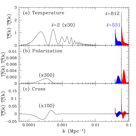
Figure 4: Spatial spectrum of an individual $\ell$ mode for a scale invariant initial spectrum. The temperature quadrupole $\ell=2$ receives ISW contributions across a wide range in $k$ while the polarization quadrupole has a much tighter distribution. At the acoustic peaks ($\ell_{m=2}=531$, $\ell_{m=3}=812$) the temperature distribution is tighter but still receives contributions around $\sim k_{m+1/2}$ due to the broad Doppler distribution. This effect is more prominent in the polarization where the peaks represent deep minima that are filled in by the projection broadened peaks.

The acoustic and projection limitations of the temperature power spectrum are largely removed with polarization information. Near the end of recombination, photon diffusion creates local quadrupolar temperature anisotropy. Thomson scattering of radiation with a quadrupolar temperature anisotropy linearly polarizes it. The acoustic polarization transfer is therefore modulated according to velocity gradients or $(k/k_{D})\sin(ks_{*})$ and like the Doppler effect is out of phase with the local temperature. Unlike the Doppler effect, the projection of polarization is sharp (see Fig. 3). The spherical decomposition of plane wave $E$-polarization projects as ZalSel97

$$j_{\ell}(kD_{*})\rightarrow\sqrt{{3\over 8}{(\ell+2)!\over(\ell-2)!}}{j_{\ell}(kD_{*})\over{(kD_{*})^{2}}}\,,$$ (10)

leading to a nearly diagonal transfer function (see Fig. 1). Furthermore there is only one source of acoustic polarization unlike the temperature and so the power spectrum in $k$ space $\Delta^{2}_{E}(k)$ possesses zeros at $k_{m}$, where $m$ is an integer. These sharp features in $k$ are only moderately smoothed by the projection. Finally the low $k$, low $\ell$ end of the polarization transfer function is dominated by rescattering during reionization. The projection remains fairly sharp in comparison to the ISW dominated temperature projection though the shorter distance to the reionization epoch leads to a slightly larger $\ell$ for a given $k$.

In summary, the temperature and polarization fields are complementary in the transfer function, both in the out-of-phase acoustic power in $k$ and in the sharpness of the geometric projection to $\ell$. With both spectra and the cross correlation, there is high sensitivity to the initial power spectrum in the whole acoustic range $k\sim 0.02-0.2$ Mpc^-1 with projection limiting the sharpness of features in $\ell$ to $\Delta\ell\gtrsim 10-20$. The reionization bump in the polarization also offers a cleaner probe of the long wavelength modes. Although it is still severely limited by cosmic variance and the determination of the reionization history from smaller scale modes, polarization can in principle provide an incisive test for long wavelength power in our horizon volume. It can then determine whether the anomalously small low order temperature multipoles found by COBE and WMAP are due to a lack of long wavelength power in our horizon volume or a chance cancellation with more local effects.

III Discrete Representation and Gravitational Lensing

Due to the geometric projection and, as we shall see, gravitational lensing, sharp features in the initial power spectrum will not be preserved in the observable angular power spectra. For these reasons the transfer function cannot be inverted directly to obtain the initial power spectrum from the measured angular power spectra even with perfect measurements. Furthermore, as we shall see in the next section, the transfer function itself depends on cosmological parameters that must be jointly estimated from the data.

Given the physical limitations of the transfer function it is convenient to represent the initial power spectrum by a discrete set of parameters. This discretization will also facilitate the treatment of gravitational lensing below. Specifically, we represent the initial power spectrum as

$$\ln\Delta_{\zeta}^{2}(k)=\ln\delta_{\zeta}^{2}+\sum_{i}p_{i}W_{i}(\ln k)\,,$$ (11)

where $W$ is the triangle window

$$W_{i}(\ln k) = {\rm max}\left(1-\big{|}{\ln k-\ln k_{i}\over\Delta\ln k}\big{|},0\right)\,,$$ (12)

and we have assumed a constant

$$\Delta\ln k=\ln k_{i+1}-\ln k_{i}\,.$$ (13)

The parameters $p_{i}$ then represent perturbations about the fiducial scale invariant model with $\delta_{\zeta}=5.07\times 10^{-5}$. An arbitrary initial power spectrum is then represented as the linear interpolation in a log-log plot of points sampled at $k_{i}$. If the initial power spectrum contains features below the sampling rate then the points represent averages through the windows. This parameterization preserves the positive definiteness of the initial power spectrum at the expense of making the initial power spectrum non-linear in the parameters.

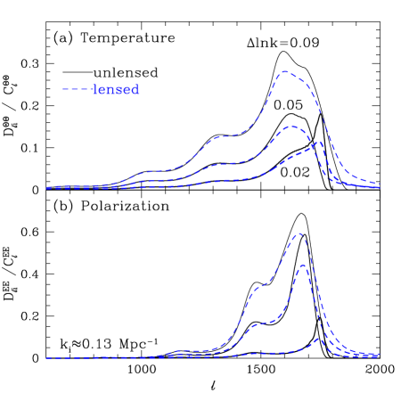
Figure 5: The power spectrum transfer matrix $D_{\ell i}^{XX}$ of a discrete perturbation in the initial power spectrum at $\ln k_{i}$ of width $\Delta\ln k$. Here $k_{i}\approx k_{m=6}\approx 0.13$ Mpc^-1. The transfer is broadened by projection and lensing such that only features of $\delta k/k>0.05$ can be resolved.

We can now define the infinitesimal response in the observable power spectra to the initial power parameters

$$D_{\ell i}^{XX^{\prime}} = {\partial C_{\ell}^{XX^{\prime}}\over\partial p_{i}}\big{|}_{\rm fid}$$

$$= {2\pi\over\ell(\ell+1)}\int d\ln k\,T^{X}_{\ell}(k)T^{X^{\prime}}_{\ell}(k)\,\delta_{\zeta}^{2}W_{i}\,.$$

This response function is a true transfer matrix for small perturbations $p_{i}$ from the fiducial model,

$$C_{\ell}^{XX^{\prime}}\approx C_{\ell}^{XX^{\prime}}\big{|}_{\rm fid}+\sum_{i}D_{\ell i}^{XX^{\prime}}p_{i}\,.$$ (15)

In Fig. 5 (solid lines) we show this transfer matrix for three choices of $\Delta\ln k=0.09$, $0.05$ and $0.02$ and $k_{i}\approx k_{m=6}\approx 0.13$ Mpc^-1. Note that the intrinsic resolution from the projection is only being reached at the finest binning for this high a $k$.

The necessity of fine binning at high $k$ reflects a trade-off in the choice of parameterization of the initial power spectrum. A logarithmic parameterization facilitates working with traditional approaches. Inflationary deviations from scale-invariance are usually quantified by the tilt $n$ and its running $\alpha$

$$\ln\Delta_{\zeta}^{2}(k) = \ln\delta_{\zeta}^{2}+(n-1)\ln({k\over k_{0}})+{1\over 2}\alpha\ln^{2}({k\over k_{0}})\,.$$ (16)

Thus the traditional parameterization is a Taylor expansion in log-log space around the pivot point $\ln k_{0}$. As a Taylor expansion, this parameterization can only be extended to a large dynamic range $\Delta\ln(k/k_{0})>1$ if $\alpha\ll(1-n)\ll 1$ and can yield misleading results if extended beyond its regime of applicability. Nevertheless, the effect of $n$ and $\alpha$ can be easily constructed from the discrete parameters

$$p_{i} \approx (n-1)\ln({k_{i}\over k_{0}})+{1\over 2}\alpha\ln^{2}({k_{i}\over k_{0}})\,,$$ (17)

to high accuracy with logarithmically spaced modes.

The drawback of a logarithmic representation is that the geometric projection causes a smoothing that is roughly linear in $\ell$ and hence the minimum $\Delta\ell/\ell$ of features decreases with $\ell$. However there is a second fundamental limitation on features in the power spectrum that takes over at high $\ell$: gravitational lensing Sel96b .

Gravitational lensing deflects each line of sight according to the angular gradient in the projected potential $\phi$

$${\hat{\bf n}} \rightarrow {\hat{\bf n}}+\nabla\phi({\hat{\bf n}})\,,$$

$$\phi({\hat{\bf n}}) = 2\int dD_{c}{D_{*}-D\over D_{*}D}\Phi({\bf x}={\hat{\bf n}}D,D_{c})\,,$$ (18)

where the conformal lookback time $D_{c}=D$ in the flat fiducial model. $\Phi$ is the Newtonian curvature and it is related to the density perturbation in the comoving gauge by the Poisson equation. In the fiducial cosmology, an rms deflection of $\sigma_{d}\approx 3^{\prime}$ arises from the projected potential

$$\sigma_{d}^{2}=\sum_{\ell}\ell(\ell+1){2\ell+1\over 4\pi}C_{\ell}^{\phi\phi}$$ (19)

and gets its main contributions from $\ell\sim 50$. In other words, the arcminute scale deflections have a coherence of several degrees. Also important are the fluctuations at the arcminute scale which cause a deflection of a few arcseconds.

Following the linearized all-sky harmonic approach Hu00b , the change in the observed power spectrum is

$$\delta C_{l}^{XX^{\prime}} = -[\ell(\ell+1)-{s_{X}^{2}+s_{X^{\prime}}^{2}\over 2}]{\sigma_{d}^{2}\over 2}C_{\ell}^{XX^{\prime}}$$

$$\quad+\sum_{\ell_{1}\ell_{2}}C_{\ell_{1}}^{\phi\phi}C_{\ell_{2}}^{XX^{\prime}}({}_{s_{X}}M_{\ell\ell_{1}\ell_{2}})({}_{s_{X^{\prime}}}M_{\ell\ell_{1}\ell_{2}})\,,$$

where $s_{\Theta}=0$ and $s_{E}=2$ and the mode coupling term

$${}_{s}M_{\ell\ell_{1}\ell_{2}} = {1\over 2}[\ell_{1}(\ell_{1}+1)+\ell_{2}(\ell_{2}+1)-\ell(\ell+1)]$$ (24)

$$\times\sqrt{(2\ell_{1}+1)(2\ell_{2}+1)\over 4\pi}\left(\begin{array}[]{ccc}\ell&\ell_{1}&\ell_{2}\\ s&0&-s\\ \end{array}\right)\,,$$

if $\ell+\ell_{1}+\ell_{2}=$ even; 0 if odd.

This mode coupling leads to a broadening of features in the angular power spectra in two ways. The main effect is a large-angle warping of the temperature and polarization maps that does not change the overall power in sub-degree scale fluctuations. Here the two terms in Eqn. (III) mainly cancel and the linearized approximation retains validity beyond $\ell^{2}\sigma_{d}^{2}/2=1$ except for unphysical spectra with features of $\delta\ell\sim 1$ Sel96b . However they induce a smoothing effect on features in the angular power spectrum and hence place a limit on resolving features in the initial curvature spectrum. In the absence of lensing, the resolution in harmonic space $\Delta\ell$ is set by the fundamental mode of the survey, i.e. for the full sky $\Delta\ell=1$. In the presence of lensing, the incoherence of the deflections in patches subtending more than a few degrees effectively prevents their mosaicing to achieve higher resolution. This effect places a resolution limit of $\Delta\ell\sim 50$ for the modes $\ell\gtrsim 10^{3}$ for which arcminute scale deflections are important. Thus a sampling rate of $\Delta\ln k=0.05$ is sufficient even on these scales.

The second effect is from the smaller deflections with arcminute scale coherence. These induce additional arcminute scale fluctuations from the distortion of primary fluctuations on larger scales Zal00 . In the fiducial model, this secondary power becomes comparable to the primary power in temperature at $\ell_{\rm sec}\approx 3000$ and essentially eliminates the primary information on the initial power spectrum beyond $k\gtrsim\ell_{\rm sec}/D_{*}\approx 0.02$ Mpc^-1. Thus a sampling rate of $\Delta\ln k=0.05$ suffices for the whole observable regime.

On the other hand the lensing potential power spectrum $C_{\ell}^{\phi\phi}$ is also a source of information about the curvature fluctuations at late times. Unfortunately due to the projection in Eqn. (18), lensing has little ability to distinguish sharp features in the initial power spectrum and even the interpretation of broadband power depends on the dark-energy and massive-neutrino dependent growth rate of structure KapKnoSon03 . We ignore the information here by neglecting the sensitivity to the parameters coming from $\partial C_{\ell}^{\phi\phi}/\partial p_{i}$ and the information in the $B$-mode polarization. In this approximation, derivatives of the lensed CMB power spectra in Eqn. (III) are simply given by the lensing of the power spectrum derivatives calculated from the transfer functions. In Fig. 5 (dashed lines) we show the effect of gravitational lensing on the power transfer. Now even features with $\Delta\ln k=0.05$ are limited by lensing. We will hereafter adopt this spacing as the fiducial choice which leads to 200 parameters for the initial power spectrum.

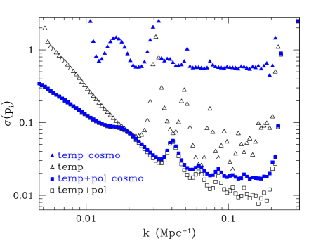
Figure 6: Individual errors on the discretized initial power spectrum $p_{i}$ with $\Delta\ln k=0.05$ and a cosmic variance limited measurement out to $\ell_{\rm sec}=3000$. With fixed cosmological parameters, temperature information alone (open triangles) recovers $p_{i}$ for modes near the acoustic peaks but not the troughs. Adding polarization information improves coverage to the whole acoustic range $k=0.02-0.2$ Mpc^-1 (open squares). Adding cosmological parameters destroys individual parameters constraints with just temperature information (filled triangles) which are largely recovered by adding polarization information (filled squares). Much of the constraining power is hidden in the strongly anticorrelated covariance (not shown).

IV Statistical Forecasts and Cosmological Parameters

A third limitation on the recovery of the initial power spectrum comes from degeneracy with cosmological parameters such as the energy density of the particle constituents of the universe today. We employ the Fisher matrix technique to study the effect of degeneracies. Construction of the Fisher matrix will also be the first step in building statistics that are immune to cosmological parameter uncertainty.

We begin by appending the $n_{c}$ cosmological parameters to the initial power vector $p_{i}$ to form the joint parameter vector $p_{\mu}$, $\mu=1,\ldots,n_{k},\ldots,n_{k}+n_{c}$. The Fisher matrix for a cosmic variance limited measurement out to $\ell=\ell_{\rm sec}$ is

$$F_{\mu\nu}=\sum_{\ell=2}^{\ell_{\rm sec}}{2\ell+1\over 2}{\rm Tr}[{\bf D}_{\ell\mu}{\bf C}_{\ell}^{-1}{\bf D}_{\nu\ell}{\bf C}_{\ell}^{-1}]\,,$$ (25)

where we have suppressed the $XX^{\prime}$ indices in a matrix notation for the derivatives and the power; here

$$({\bf D}_{\ell\mu})_{XX^{\prime}}=D_{\ell\mu}^{XX^{\prime}}\equiv{\partial C_{\ell}\over\partial p_{\mu}}$$ (26)

is the generalization of the transfer matrix Eqn. (III). Given gravitational lensing constraints and other sources of foreground contamination, we will take $\ell_{\rm sec}=3000$.

The inverse Fisher matrix approximates the covariance matrix of the parameters. In particular, the marginalized 1-$\sigma$ errors on a given parameter $\sigma(p_{\mu})$ are given by

$$\sigma^{2}(p_{\mu})=C_{\mu\mu}\approx({\bf F}^{-1})_{\mu\mu}\,.$$ (27)

The Fisher matrix also allows for a simple conversion between representations of the parameter set $p_{a}$ and $p_{\mu}$

$$F_{\rm ab}=\sum_{\mu\nu}{\partial p_{\mu}\over\partial p_{a}}F_{\mu\nu}{\partial p_{\nu}\over\partial p_{b}}\,,$$ (28)

where $p_{a}$ can have a lower dimensionality, e.g. by going from the initial power parameterization of $p_{i}$ to $n$ and $\alpha$ through Eqn. (17).

In Fig. 6, we show the statistical errors on the initial power spectrum parameters $p_{i}$. Even in the absence of cosmological parameters ($n_{c}=0$) the constraints on the $p_{i}$ are strongly modulated by the acoustic oscillations with temperature information alone. The $k$-modes associated with the acoustic troughs (half integral $m$) are poorly constrained while those associated with the peaks (integral $m$) are fairly well constrained. For low $k$, both the projection and cosmic variance severely limits the resolution in $k$ leading to a strong anticorrelation between points. Hence only broadband power and not features can be recovered. For $k>0.2$ Mpc^-1 the cut off at $\ell_{\rm sec}=3000$ limits the information.

With the addition of the polarization and cross spectra information, the modulation of errors with the peaks reverses. Now modes associated with acoustic troughs are better constrained than those associated with the peaks. The polarization information becomes even more important once the cosmological parameters are added back in. In Fig. 6 we take 6 additional parameters $\Omega_{b}h^{2}$, $\Omega_{m}h^{2}$, $\Omega_{\rm DE}$, $w$, $\tau$ and $r$, where $r$ is the tensor-scalar ratio. With temperature information alone, the ability to measure an individual $p_{i}$ is essentially completely destroyed since the response to a cosmological parameter can always be mimicked by a particular superposition of $p_{i}$’s Kin01 . However only six such combinations are lost and so with the addition of polarization information with its complementary transfer function, the effect of marginalizing cosmological parameters is fairly small. In fact even with temperature information alone, there are modes that are very well constrained. The raw marginalized errors on $p_{i}$ are misleading in that they do not show the covariance. It is therefore useful to find a more efficient representation of the information that accounts for projection, lensing and cosmological parameters.

Figure 7: First 5 principal components of the covariance matrix with 6 cosmological parameters, the amplitude $\ln\delta_{\zeta}$ and tilt $n$ marginalized. The modes are normalized to unit variance over $d\ln k$ (discretized to $\Delta\ln k=0.05$). Well-constrained modes are localized in the acoustic regime $k=0.02-0.2$ Mpc^-1 and give zero weight to scale-free deviations.

V Principal Components and Deviated Spectrum

Figure 8: Eigenvalues and cumulative constraints on the running of the tilt $\alpha$ represented in modes. For cosmic variance limited temperature and polarization measurements out to $\ell_{\rm sec}=3000$, approximately 50 modes can be measured to percent level precision ($\sigma(m_{a})<0.01$). Information on the running $\alpha$ saturates with more that $\sim 10$ modes.

Given the limitations imposed by projection, lensing and cosmology what kinds of deviations from a scale-free initial spectrum can the CMB best probe? To answer this question, we now consider a principal component representation of features.

The information retained after including these three effects is quantified by the covariance matrix of the deviation parameters $p_{i}$, the $C_{ij}$ subblock of the joint covariance matrix $C_{\mu\nu}$. Employing the Fisher matrix approximation of the last section, we can determine the principal component representation based on the orthonormal eigenvectors $S_{ia}$ of $C_{ij}$

$$C_{ij}=A^{-2}\sum_{a}S_{ia}\sigma_{a}^{2}S_{ja}\,,$$ (29)

where $A$ is a normalization parameter. For a fixed $a$, $S_{ia}$ specifies a linear combination of the deviation parameters $p_{i}$ for a new representation of the spectrum

$$m_{a}=A\sum_{i}S_{ia}p_{i}\,,$$ (30)

where the covariance matrix of the mode amplitudes is given by

$$\left<m_{a}m_{b}\right>=\sigma_{a}^{2}\delta_{ab}\,.$$ (31)

This relationship can also be derived from Eqn. (28). In other words, the eigenvectors form a new basis that is complete and yields uncorrelated orthogonal measurements with variance given by the eigenvalues. We choose the normalization $A=(\Delta\ln k)^{-1/2}$ so that a $m_{a}=1$ corresponds to a deviation with unit variance when integrated over $d\ln k$, i.e.

$$A^{2}\int{d\ln k}\,S_{ia}^{2}\approx\sum_{i}S_{ia}^{2}=1\,.$$ (32)

Modes corresponding to combinations that are degenerate with cosmological parameters or due to the projection and lensing have high eigenvalues and high variances and may be removed without loss of information.

In Fig. 7, we show the first five eigenvectors of the covariance matrix including both temperature and polarization information. In this case we append $\ln\delta_{\zeta}$ (or $\ln A$) and $n$ to the list of cosmological parameters included in §IV. By doing so, the best constrained eigenvectors automatically null out changes in the amplitude and tilt and so can be interpreted as the best modes to search for deviations from scale-free initial conditions. They also tend to null out any slowly varying component from residual secondary effects and foregrounds. As a consequence, their form is similar to Fourier modes confined to the well-measured acoustic regime $0.02-0.2$ Mpc^-1 with the constant and gradient term (in $\ln k$) removed. For the cosmic variance temperature and polarization spectra assumed in the Fisher matrix calculation, the mode errors are shown in Fig. 8 (solid line) and remain below the percent level for $\sim 50$ modes.

Note that truncation of the eigenmodes does not limit types of initial spectra that can be tested against the measurements $m_{a}$ since any spectrum may be projected onto the measurement basis. As an example, consider constraints on a constant running of the tilt $\alpha$ in the measurement basis. Each mode independently measures $\alpha$ with a variance

$$\sigma_{a}^{2}(\alpha)=A\sum S_{ia}{1\over 2}\ln^{2}({k_{i}\over k_{0}})\,,$$ (33)

where the pivot $k_{0}$ is arbitrary since the $S_{ia}$ null out a constant deviation. Since each measurement is independent, the total variance is given by

$${1\over\sigma^{2}(\alpha)}=\sum_{a=1}^{a_{\rm max}}{1\over\sigma^{2}_{a}(\alpha)}\,.$$ (34)

This cumulative sum is shown in Fig. 8 (dashed line). Information on $\alpha$ is efficiently captured in the first 10 eigenmodes.

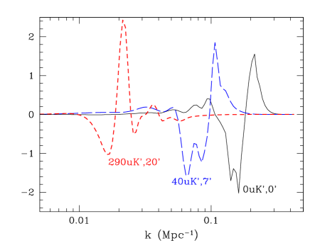
Figure 9: Eigenvectors in the presence of instrumental noise (in $\mu$K-arcmin) and beam (FWHM in arcmin). Parameters are chosen to roughly bracket the expectations of WMAP and Planck (dashed lines) for comparison with the noise-free case (solid lines). The eigenvectors are now confined to $\ell$-modes and hence $k$-modes that are larger than the beam. In the highest noise, large beam case, polarization information is degraded and the avoidance of cosmological parameter degeneracies complicates the mode structure.

The principal component technique can be made into a practical tool for searches for deviations from scale-free initial curvature fluctuations. The best measured modes are fairly smooth and take forms that are independent of the discretization $\Delta\ln k$ of the underlying representation. Hence they may be replaced by a continuous representation for parameter estimation with an efficient integral code such as CMBFast or CAMB. The parameters $m_{a}$ can then be added in the usual way to a Monte Carlo Markov Chain. Deviations of the true model from the assumed fiducial model in constructing the eigenmodes and non-linearities in the parameter dependence will degrade the statistical orthogonality of modes implied by Eqn. (31). These covariances will nonetheless be captured in the likelihood exploration. The process may also be iterated if the assumed eigenvectors deviate substantially from those of the best fit cosmology.

Furthermore, although we have assumed a perfect experiment here to determine the limitations imposed by physical processes on feature recovery, the techniques are readily optimized for specific experiments. One simply replaces the power spectra in Eqn. (25) for the Fisher matrix with the total signal and noise power spectra of a given experiment. In Fig. 9, we show a simple example where the experiment is parameterized by a white noise level in $\mu$K-radian $\Delta T$ and the FWHM of a Gaussian beam $\theta$. Here

$$C_{\ell}^{\Theta\Theta}\big{|}_{\rm noise} = ({\Delta T\over T})^{2}e^{\ell(\ell+1)\theta^{2}/8\ln 2}\,,$$

$$C_{\ell}^{EE}\big{|}_{\rm noise} = 2({\Delta T\over T})^{2}e^{\ell(\ell+1)\theta^{2}/8\ln 2}\,,$$

$$C_{\ell}^{\Theta E}\big{|}_{\rm noise} = 0\,.$$ (35)

We show the best eigenmode for two examples that roughly bracket the expectations for the completed WMAP and Planck missions. Note that the main effect is to replace the cutoff imposed by $\ell_{\rm sec}$ with that of the beam. However the smaller $\ell$ range and the loss of polarization in the high noise example complicate the form of the mode because it adjusts to remain orthogonal to the cosmological parameters.

VI Discussion

Physical limitations imposed by the formation and evolution of CMB temperature and polarization anisotropy limit the ability to recover the initial power spectrum from even perfect measurements of angular power spectra. The initial power spectrum can be well measured in the acoustic regime $k=0.02-0.2$ Mpc^-1 but projection and gravitational lensing prevents resolution of features smaller than $\Delta k/k\approx 0.05$. The complementary acoustic polarization information greatly assists in filling in the coverage near the acoustic troughs and in immunizing the determination to cosmological parameter degeneracies. Furthermore polarization in principle offers a cleaner probe of long-wavelength power through reionization effects. Beyond purely two-point statistics in the temperature and polarization fields, the limitations of gravitational lensing can in principle be removed HuOka01 ; HirSel03 . This can moderately improve the resolution of features but will only be possible with ultra-high precision polarization measurements across nearly the whole sky.

We have constructed the best statistics for measuring deviations from scale-free initial conditions given these physical limitations on power spectra. They are constructed from the principal components of the covariance matrix. These modes resemble a Fourier expansion of the initial spectrum that is localized to the acoustic regime. Approximately 50 modes in this regime ultimately can be measured with percent level precision. These modes can provide many independent measurements of model-motivated parameters such as the running of the tilt as a consistency check that such simpler parameterizations are adequate.

Although beyond the scope of this work, the principal component technique can be developed into a practical tool for the search for deviations from scale-free conditions with current experiments. These may also include non-CMB sources with the appropriate addition of Fisher matrices. Here the physical limitations imposed on the modes would be supplemented by experimental limitations. The principal component technique provides a general, physically-motivated and complementary tool for the study of the initial power spectrum and its implications for early universe physics.

Acknowledgments: This work was supported by NASA NAG5-10840 and the DOE OJI program. We thank the Aspen Center for Physics and the participants of the CMB workshop, epecially endgamers S. Bridle, M. Kaplinghat, A. Lewis, S. Myers, B. Wandelt, and Y. Wang.

References

- (1)
- (2) H.V. Peiris, et al. Astrophys. J, submitted, astro-ph/0302225 (2003). WMAP normalization .
- (3) http:astro.estec.esa.nl/Planck
- (4) http://universe.gsfc.nasa.gov/be/roadmap
- (5) V.F. Mukhanov, H.A. Feldman and R.H. Brandenberger, Phys. Rept., 215, 203 (1992); A.R. Liddle and D.H. Lyth, Phys. Rept., 231, 1 (1993).
- (6) P. Mukherjee and Y. Wang, Astrophys. J, submitted, astro-ph/0303211 (2003); Y. Wang and G. Mathews, Astrophys. J, 573, 1 (2002); Y. Wang, D.N. Spergel and M.A. Strauss, Astrophys. J, 510, 20 (1999).
- (7) C.J. Miller, R.C. Nichol, C. Genovese and L. Wasserman, Astrophys. J, 565, 67 (2002).
- (8) M. Tegmark and M. Zaldarriaga, Phys. Rev. D, 66, 103508 (2002).
- (9) S.L. Bridle, A.M. Lewis, J. Weller and G. Efstathiou, Mon. Not. R. Astron. Soc., submitted, astro-ph/0302306 (2003).
- (10) M. Zaldarriaga and U. Seljak, Phys. Rev. D, 55, 1830 (1997). Note the opposite sign convention for follows W. Hu and M. White, Phys. Rev. D, 56, 596 (1997).
- (11) W. Hu and N. Sugiyama, Phys. Rev. D, 51, 2599 (1995); W. Hu and N. Sugiyama, Astrophys. J, 444, 489 (1995).
- (12) U. Seljak and M. Zaldarriaga, Astrophys. J, 469, 437 (1996).
- (13) A. Lewis, A. Challinor and A. Lasenby, Astrophys. J, 538, 473 (2000).
- (14) M.L. Wilson and J. Silk, Astrophys. J, 243, 14 (1981).
- (15) J.R. Bond and G. Efstathiou, Astrophys. J, 285, 45 (1984).
- (16) M. White and D. Scott, Astrophys. J, 459, 415 (1996).
- (17) W. Hu, D. Scott, N. Sugiyama and M. White, Phys. Rev. D, 52, 5498 (1995).
- (18) W. Hu, U. Seljak, M. White and M. Zaldarriaga, Phys. Rev. D, 57, 3290 (1998).
- (19) S. Seager, D.D. Sasselov and D. Scott, Astrophys. J, 523, 1 (1999).
- (20) U. Seljak, N. Sugiyama, M. White and M. Zaldarriaga, Phys. Rev. D, submitted, astro-ph/0306052 (2003).
- (21) R.K. Sachs and A.M. Wolfe, Astrophys. J, 147, 73 (1967).
- (22) J.R. Bond and G. Efstathiou, Mon. Not. R. Astron. Soc., 226, 655 (1987).
- (23) W. Hu and M. White, Astrophys. J, 479, 568 (1997).
- (24) U. Seljak, Astrophys. J, 463, 1 (1996).
- (25) W. Hu, Phys. Rev. D, 62, 043007 (2000).
- (26) M. Zaldarriaga, Phys. Rev. D, 62, 063510 (2000).
- (27) M. Kaplinghat, L. Knox and Y.S. Song, Phys. Rev. Lett., submitted, astro-ph/0303344 (2003); W. Hu, Phys. Rev. D, 65, 023003 (2002);
- (28) W.H. Kinney, Phys. Rev. D, 63, 043001 (2001).
- (29) W. Hu and T. Okamoto, Astrophys. J, 574, 566 (2002).
- (30) C.M. Hirata and U. Seljak, Phys. Rev. D, submitted, astro-ph/0306354 (2003).