Optical-Infrared ANDICAM Observations of the Transient Associated with GRB 030329

Abstract

We present photometry of the transient associated with GRB 030329 obtained with the CTIO 1.3–meter telescope and the ANDICAM instrument, a dual optical/infrared imager with a dichroic centered at one micron. Without the need for light curve interpolation to produce snapshot broadband spectra, we show that the transient spectrum remained statistically achromatic from day 2.7 to day 5.6, during a re-brightening episode. Associating the light in these early epochs with the GRB afterglow, we infer a modest level of extinction due to the host galaxy in the line–of–sight toward the GRB: $A_{V}$(host) = $0.30\pm 0.03$ mag for $\beta=-0.5$ and $A_{V}$(host) $<0.4$ mag (3 $\sigma$) for any physically plausible value of $\beta$ (with flux $f_{\nu}\propto\lambda^{-\beta}$). We conclude that the spectral slope of the afterglow component was more than $\beta=-$0.8 between day 2.7–5.6 after the GRB, excluding the possibility that the synchrotron cooling break passed through the optical/IR bandpass over that period. Taking extinction into account, a decomposition of the light curve into an afterglow and supernova component requires the presence of a supernova similar to that of SN 1998bw, an afterglow that shows some evidence for a second break around day 8–10, and a fifth re-brightening event around day 15. Assuming an SN 1988bw-like evolution and a contemporaneous GRB and SN event, the peak SN brightness was $M_{V}=(-19.8\pm 0.4)-5\,\log_{10}h_{65}$ mag.

1 Introduction

The low redshift long-duration cosmological $\gamma$-ray burst, GRB 030329 (Vanderspek et al., 2003) afforded an unprecedented glimpse into the aftermath of the explosion. The sheer brightness of the early optical afterglow (Peterson & Price, 2003; Torii, 2003) allowed for high-precision ($\sim 1-5$%) photometric measurements to be obtained from a bevy of meter-class telescopes (Uemura et al., 2003; Burenin et al., 2003; Rykoff & Smith, 2003; Price et al., 2003a; Lipkin et al., 2003b). The optical light curve exhibited 10–30% brightness undulations during the first several hours (Uemura et al., 2003) and then showed a prominent break at day 0.48 (Garnavich et al., 2003b; Price et al., 2003b). Later, the optical transient underwent a brightness resurgence (at about day 2) followed by an overall decline that was punctuated by four major re-brightening episodes (Li et al., 2003; Lipkin et al., 2003a, c; Sato et al., 2003; Granot et al., 2003).

Beginning about 6 days after the burst, the first signs of an underlying supernova (SN) component began to emerge in the transient, both spectroscopically (Stanek et al., 2003; Chornock et al., 2003; Hjorth et al., 2003; Kawabata et al., 2003) and photometrically (Henden et al., 2003; Matheson et al., 2003); the SN was designated by the IAU as SN 2003dh (Garnavich et al., 2003a). The evolution of the SN spectrum in the first two months closely parallels that of the bright type Ic SN 1998bw (Galama et al., 1998; Patat et al., 2001) thus confirming the previous evidence for (nearly) contemporaneous SN and GRB events from the same progenitor in other bursts (see Bloom 2003 for review).

While the nature of the SN associated with GRB 030329 is, of course, of intense interest, a detailed study of the afterglow holds potential for insight into the structure of GRB explosions. It is standard practice to model the afterglow as arising from a jetted point explosion in a constant density environment (e.g., Rhoads, 1997; Sari et al., 1998) or a wind-stratified circumburst medium (e.g., Chevalier & Li, 1999). However, the assumption of an instantaneous explosion with a constant jet opening angle is untenable both on theoretical grounds and empirical grounds. In particular, strong variations have been seen in the early afterglows of GRBs, e.g., GRB 021004 (Fox et al., 2003) and GRB 030329 (Price et al., 2003b; Uemura et al., 2003; Burenin et al., 2003; Rykoff & Smith, 2003; Price et al., 2003a).

These re-brightenings in GRB 030329 require energy addition to the radiating front. The energy addition can be due to slower moving ejecta shells colliding with the earlier emitted but faster moving ejecta (Granot et al., 2003); such a hypothesis was first proposed for the variability in GRB 021004 (Fox et al., 2003). An alternative interpretation is that the energy addition is due to shells with larger opening angles but with slower moving ejecta (Berger et al., 2003). The placement of the behavior of the late-time afterglow light curve of GRB 030329 in the context of radio modeling can help distinguish between these two hypotheses (Berger et al., 2003).

An understanding of the multitude of physical processes contributing to the complex behavior of the transient requires a careful treatment of the high-quality data. Although analysis of the vast follow-up data on GRB 030329 in the literature will no doubt be of great use, we have chosen to focus on optical-IR photometric data obtained from the same telescope and reduced uniformly. Whereas the burst has been studied extensively at optical wavelengths, only one other study presents photometric data in the near-infrared (Matheson et al., 2003). Extending the wavelength coverage by a factor of two allows stronger constraints to be placed on the extinction, and a better determination of the slope of the afterglow spectrum as a function of time.

In §2, we present the optical and infrared data obtained with ANDICAM between day 2 and day 23 after the GRB trigger. To disentangle the various physical components of the transient light, in §3 we first show that while the overall source brightness fluctuated in the first 6 days, the spectrum of the transient remained fixed. In §3.1, we then fit this early spectrum to find a constraint on the line–of–sight extinction to the GRB and the intrinsic afterglow spectrum. Using these values, we then decompose the afterglow and the supernova light in §3.2. We compare our results to those obtained in other studies and conclude with some implications for the GRB–supernova connection and the explosion structure of GRB 030329.

2 Observations, Reductions, and Calibrations

All the observations reported herein were carried out with the ANDICAM instrument mounted on the 1.3-m telescope at Cerro Tololo Interamerican Observatory (CTIO). The ANDICAM is a dual-channel camera constructed by the Ohio State University instrument group. The camera contains a dichroic that enables two imagers to be simultaneously illuminated: a Rockwell 1024$\times$1024 HgCdTe “Hawaii” array, and a Fairchild 447 2048$\times$2048 optical CCD. This instrument was formerly mounted on the Yale 1-m telescope at CTIO, operated by the YALO consortium (Bailyn et al., 1999). ANDICAM has recently been transferred to the 1.3-m telescope at CTIO, formerly used for the 2MASS survey, where it has been operating since February 2003 by the SMARTS consortium. The image scale is smaller at the 1.3-m than it was at the 1-m, and the field of view is now 2.4^′$\times$2.4^′ for the IR array, and 6.3^′$\times$6.3^′ for the CCD. The optical images are routinely double binned to provide a pixel scale of 0.37^′′/pixel, while the IR channel significantly oversamples the seeing (typically 0.8^′′) with 0.14^′′ pixels.

The field seen by the IR array can be repositioned slightly by adjusting three tilt axes of an internal mirror. This allows us to “dither” the IR position while an optical integration is underway. These dithered IR images can be used to generate a sky image without actually moving the telescope. Such sky images are slightly inferior to those made by moving the telescope, since the field is viewed through a different part of the filter, leading to decreased accuracy in flat fielding. This problem is most significant in the $K$-band, which, at the 1.3-m, also suffers from high background levels.

Table 1 gives a log of the observations with ANDICAM. The data have been grouped into 13 individual epochs. As can be seen the total duration of the epochs was always less than 40 minutes, even over epochs where $BVIJH$ images were acquired. Individual optical images were reduced using IRAF/CCDRED. The bias was removed using a mean of several bias frames and the images then flat-fielded using the best composite twilight flats for the appropriate filter. Twilight flats were not obtained on every night of the transient observations but the differential gain variations over several days should not affect the photometric uncertainty at significantly more than the 1% level. Images where the OT light was contaminated with cosmic rays were excluded from the final sample.

Individual infrared images were reduced in the following way. Flat fields were created in $J$- and $H$-bands by subtracting pairs of twilight flats with different sky brightnesses. After dark subtraction each science frame was divided by the (normalized) flat field. Next, a sky frame was created by taking the median of all normalized images for a given epoch, and subtracted after rescaling to match the counts in the original images. In the $H$- and $K$-bands strong “ripples” are present in the reduced images. These features likely result from the ANDICAM dithering mode: as mentioned, at each mirror position the light passes through a different part of the filter, creating residual flat fielding errors. In the $H$-band the features could be successfully removed by creating residual flat fields, created from all images (at all epochs) taken at the same mirror position. In the $K$-band the residual pattern dominated the flux of the transient even after this correction; therefore, the $K$-band observations are not considered further in this paper. Finally, for both the optical and IR images, cosmic-rays were removed using a Laplacian edge-detection algorithm (van Dokkum, 2001).

Usually only one or two images per epoch were obtained per optical filter, while each epoch generated between 7–21 dithered images per IR filter. In a given IR image, often only a few objects were detected at better than 3 $\sigma$, requiring a complicated image alignment procedure in order to stack the images. In a custom Pyraf code, we first removed any large scale gradient from a copy of all the images using IRAF/MKSKYFIT, masked hot and cold pixels, and then smoothed these images with a Gaussian of width 3 pixels. The pixel–to–pixel rms was then determined using an iterative sigma-clipping algorithm. This rms was then used as an input to DITHER/PRECOR to mask out all regions of the sky where less than 18 out of the neighboring 5$\times$5 pixels were above three times the rms. The effect was to create masked images where only objects appear, and the remainder of the pixels are set to zero.

An initial estimate of the true offset was computed using the positional and mirror keywords in the FITS headers. For epochs where the seven-point dither pattern was repeated at least once, we found that a given set of three mirror tilts (recorded in the FITS headers) consistently mapped source positions to better than one pixel rms. From a training set, we fit a linear least-squares transfer (3$\times$2) matrix to map the three tilts to a nominal $x,y$ source position taking into account the reported telescope pointing, plate orientation, and pixel scale; we assumed no differential sky rotation from image to image. The difference between the nominal $x,y$ position in the fiducial image and the nominal $x,y$ position in a given image yielded an estimate of the nominal offset.

To find the precise offsets between a fiducial image and the other images in a given epoch, we cross-correlated the masked images using DITHER/CROSSDRIZZLE. The highest peak in the cross correlation within a 50 pixel width box about the nominal offset position was then found and centroided using SHIFTFIND; this process yielded a list of sub-pixel offsets with uncertainties less than 0.1 pixels. Individual epochs were then stacked with DITHER/DRIZZLE using these offsets without re-sampling the data to a finer grid (i.e., drizzle.scale = 1 and drizzle.pixfrac = 1). The offsets between the stacked images of all IR epochs were then computed using the same cross-correlation technique. The final epoch stacks were made using these epoch–to–epoch offsets as input to the secondary geometry parameters for drizzle (drizzle.dr2gpar), repeating the entire process described above. The result was a set of stacked, registered images for all IR epochs.

Using IRAF/FITPARAM, we calibrated our first epoch ($t=2.67$ day) of optical images to secondary field standards reported in Henden (2003). An average extinction vs. airmass curve from nearby Paranal was assumed and the differential color terms found to be consistent with zero. This implies that our cumulative filter$+$telescope response curves reasonably approximate those of the Henden system, and thus closely resemble the Johnson BV and Kron-Cousins I filters (i.e., Landolt system). The photometry for all subsequent epochs were computed differentially from the zeropoints established on the first epoch. As a check, primary optical Landolt standard stars were observed on several different photometric nights and found to yield consistent photometry to better than 5% accuracy.

The infrared standard star SJ9144 (Persson et al., 1998) was observed on the third (photometric) epoch (April 3 UT). Using curve–of–growth aperture photometry, we determined a zeropoint for the IR science observations at that epoch and assume a systematic zeropoint uncertainty of 0.05 mag. Aperture photometry corrected to the “infinite aperture” magnitudes were computed for the transient and all detectable secondary standards in the field for all epochs. As with the optical observations, photometry was computed differentially from this fiducial epoch. The resulting photometry is given in Table 1. Note that while our $J$-band photometry agrees with the results from Matheson et al. to within the statistical uncertainties, as brought to our attention by K. Krisciunas, our $H$-band measurements appear to be about 0.2 mag fainter at similar epochs to the results in Matheson et al. Unfortunately, there are no intercomparison stars at common epochs between the two datasets. Therefore we were unable to determine the origin of the difference in the $H$-band.

Transient fluxes were first computed from the observed magnitudes assuming the transformations given in Fukugita et al. (1995) (optical) and Bessell & Brett (1988) (IR). This revealed a small and consistent curvature in the broadband spectrum in the first several epochs, with an incident spectrum ranging from $\beta\approx-1$ at the blue end to $\beta\approx-0.6$ in the red end. Since the effective wavelength and zeropoint of filters depend upon the incident spectrum we recomputed these quantities by fitting a 2nd-order polynomial to the first epoch. This fiducial spectrum was then input to IRAF/CALCPHOT, part of the STSDAS/SYNPHOT package to compute the effective wavelengths ($\lambda_{\rm eff}$) and Vega-referenced zeropoints of the filters. The difference between fiducial filter wavelengths and the effective filter wavelengths was small, a few tens of Angstroms. Though the input spectrum was seen to evolve somewhat over the course of our observations (see below), given the small changes in $\lambda_{\rm eff}$ from the fiducial values, in the subsequent analysis we fix $\lambda_{\rm eff}$ for all filters at all epochs. The resulting transient fluxes are given in the last column of Table 1.

3 Results

With dense high-precision sampling, the complexity of the early light curve of GRB 030329 was revealed. The temporal features of the early afterglow ($t<1$ day) have been described in detail elsewhere (e.g., Uemura et al., 2003; Lipkin et al., 2003a). Later time “bumps and wiggles” (or rebrightenings) are also detected in the ANDICAM light curves, shown in Figure 1.

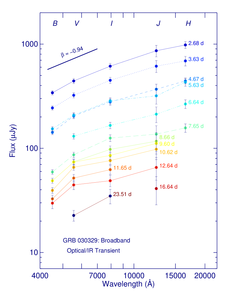
Figure 2: The broadband spectral evolution of the transient associated with GRB 030329. The time since the GRB is noted beside each spectrum. The data have not been corrected for reddening. No significant spectral evolution was detected in our first four epochs, at least until 6 days after the GRB. For reference, the initial optical spectral index reported by others ($\beta=-0.94$) is shown and is consistent with our observed spectra in the bluer filters. However, the IR data show the spectrum to flatten toward longer wavelengths, indicative of extinction due to dust reddening. A systematic uncertainty of 4% in the conversion of magnitude to flux has been included.

Figure 2 shows the transient broadband spectra over the 13 epochs of observations, uncorrected for the effects of dust reddening. As evident, while the overall brightness fluctuated (Fig. 1), there was no apparent change in the spectrum over the first several epochs. To understand the statistical significance of this apparent achromaticity, we take an empirical approach by examining the changes in the 10 color indices, constructed from the 5 observing filters (see Fig. 6). We compute the color change from the first epoch for all subsequent epochs and estimate the significance of change from the statistical errors on the measurements (i.e., only the differential errors are considered). Between epochs 1 through 4, 28 out of 30 color changes are consistent within $\pm$2 $\sigma$ from zero change; the significance of the $B-V$ and $B-I$ colors changes appears high on epoch 3 (by $3$ and $4\sigma$, respectively). From epoch 5 onward, the distribution of color change significances fans out (as will be shown in §3.2, there are also secular trends in the evolution of some colors). Specifically, the Kolmogorov-Smirnov (KS) probability that the distribution of color change significances from epochs 1–4 is drawn from a Gaussian of sigma unity centered about zero is $P_{\rm KS}=0.5$ but then plummets to below 0.05 by day 10. We therefore conclude that the transient spectrum did not begin to evolve significantly until after the fourth epoch of observations.

The lack of a significant color change in the early epochs allows us to decouple the analysis of the afterglow (dominating the first four epochs) and the supernova (contaminating the remainder of the epochs). In what follows, using the first four epochs only, we determine the intrinsic afterglow spectrum and the line–of–sight extinction concurrently. With these results, we then decompose the afterglow component and the supernova component. In accordance with early spectroscopic studies (e.g., Matheson et al. 2003), we find that any contribution to the total optical/IR light from an underlying supernova was $<5$% in all filters during the first four epochs (see §3.2).

3.1 Constraints on the Line–of–Sight Extinction

The achromaticity of the transient spectrum is consistent with the expectation of afterglow emission in the standard synchrotron shock model (e.g., Sari et al., 1998). In the model, the intrinsic optical–IR afterglow spectrum is dominated by a featureless power-law spectrum characterized as $f_{\nu}\propto\lambda^{-\beta}$. There is, however, an apparent downward curvature to the observed broadband afterglow spectrum (Fig. 2), which can modeled in the first four epochs as $f_{\nu}\approx(-3.17\pm 0.21)\lambda_{3}^{2}+(119\pm 4)\lambda_{3}-(131\pm 17)\,\mu$Jy, from $\lambda\approx 4000$ Å to 18000 Å ($\lambda_{3}\equiv\lambda/1000$ Å).

Given the expectation of an underlying power-law, the curvature is likely due to extinction by dust along the line–of–sight to the burst. We constrain the intrinsic extinction by normalizing the first four epochs to a unity flux density in $I$-band and fit the function,

$$f_{\nu}(\lambda){\rm(observed)}=C\lambda^{-\beta}\times T[R_{V}{\rm(Gal)},A_{V}{\rm(Gal)},\lambda]\times T[R_{V}{\rm(host)},A_{V}{\rm(host)},\lambda/(1+z)]\,\mu{\rm Jy},$$ (1)

where $R_{V}$ and $A_{V}$ are the extinction curves and equivalent $V$-band extinction through the Galaxy (“Gal”) and the line–of–sight through the host galaxy/progenitor system (“host”), respectively. The redshift of the host is $z=0.1685$ (Greiner et al., 2003). A parametrized transmission function $T[R_{V},A_{V},\lambda]$ is adopted from Cardelli et al. (1989).

The Galactic extinction toward the transient, estimated from Galactic foreground IR emission, is $E(B-V)=0.025$ mag (Schlegel et al., 1998). Following from a recent analysis by Burstein (2003), the statistical error on this estimate is $\sigma_{E(B-V)}\approx 0.002$ mag, or about 10%. In the extinction fit we fix $R_{V}{\rm(Gal)}=3.1$ and thus fix $A_{V}{\rm(Gal)}=0.083\pm 0.017$ mag.

By minimizing $\chi^{2}$, we first fit simultaneously for the values of $C$, $R_{V}{\rm(host)}$, $A_{V}{\rm(host)}$, and $\beta$, and found the preferred value of $R_{V}{\rm(host)}$ is small ($<2$); we consider this unlikely to be the true value of $R_{V}$ given the indication (from spectroscopy and imaging) that the host is a starburst dwarf galaxy (e.g., Matheson et al., 2003): for such galaxies we would expect an extinction curve $R_{V}\mathrel{\hbox{\hbox to0.0pt{\hbox{\lower 4.0pt\hbox{$\sim$}}\hss}\hbox{$>$}}}3$. Therefore, we examined the results for two values of $R_{V}{\rm(host)}=3.1$ and 5.1 (LMC-like). For $R_{V}{\rm(host)}=3.1$ (5.1), the best fit values are $A_{V}{\rm(host)}=0.94\pm 0.24$ mag ($1.8\pm 1.0$ mag), $\beta=0.11\pm 0.22$ ($0.5\pm 0.8$), $\chi^{2}/$dof = $0.44$ (1.34).

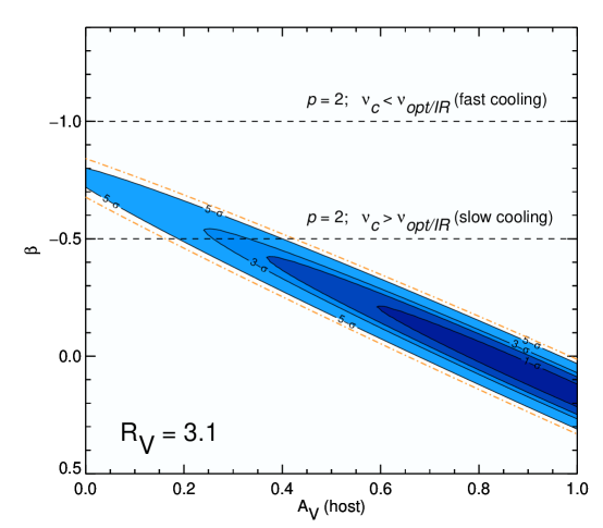
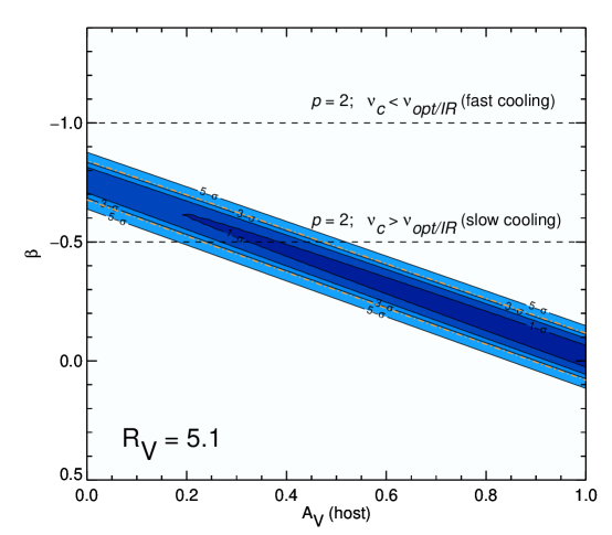
Figure 3: Coupling between the host line–of–sight restframe extinction measurement and the intrinsic spectral power-law index $\beta$ for two different extinction curves [top: $R_{\rm V}$(host)$=3.1$ (Galactic); bottom: $R_{\rm V}$(host)$=5.1$ (LMC)]. The first four epochs are used in this fit, scaled to the same flux value at the $V$-band. A Galactic extinction of $A_{\rm V}$(Gal)$=0.083$ mag, $R_{\rm V}$(Gal)$=3.1$ is assumed. Lower values of host extinction spectra result in lower (more red) values of $\beta$. The data prefer a blue afterglow with high host extinction, though physical constraints require a more red afterglow: the horizontal dashed lines show the predicted $\beta$ for $p=2$ in the fast and slow cooling regimes. For $p>2$, in either regime, $\beta$ must be more negative. Solid contours show the 1-, 2-, 3-, and 5-$\sigma$ reflect the 2-parameter demarcations from the $\chi^{2}$ surface. The dash-dotted line shows an acceptable region of the data, where $\chi^{2}$/dof $<2$. Therefore, $\beta$ must be greater than $-0.8$ in the first four epochs, ruling out the hypothesis that the cooling break, $\nu_{c}$, passed through the optical/IR bandpass between days 2 and 6.

Note that the errors given are only derived from the diagonal elements of the cross-correlation matrix. As Figure 3 demonstrates, there is a strong covariance between $A_{V}{\rm(host)}$ and $\beta$ in the sense that an intrinsically more blue afterglow requires a higher value of extinction.

Though the fits given above are formally acceptable, in both cases, the intrinsic afterglow spectrum would be unusually blue if the origin is a relativistic synchrotron shock. In previously studied afterglows, the observed temporal decline index $\alpha$ ($f_{\nu}\propto t^{\alpha}$) could be used to constrain the intrinsic spectral index through the $\alpha$–$\beta$ closure relations prescribed from synchrotron shock physics (see Price et al. 2002 and references therein). In GRB 030329, however, the complex temporal behavior does not yield an obvious estimation for the value of $\beta$. That said, if we adopt the interpretation of the light curves from Granot et al. (2003), then the temporal break observed at day $0.48\pm 0.03$ (Price et al., 2003b) can be attributed to a jet break in the standard manner, and $\beta$ then equals $-(\alpha_{2}-1)/2$. Since Price et al. (2003b) find the decay after the break to be $\alpha_{2}\approx 2$, we expect that $\beta\approx-0.5$.

A similar value (an upper limit actually) for $\beta$ is inferred by a consideration of the range of values of the electron energy index spectrum $p$, where the number density of shocked electrons as a function of energy $E$ is $n(E)\propto E^{-p}$. For the energy in the electrons to be finite, $p$ must be greater than 2. In the simplest homogeneous density model where $\nu_{c}>\nu$(opt), $\beta\leq-0.5$, consistent with value inferred above from the temporal break. The cooling frequency $\nu_{c}$ corresponds to an energy at which electrons have radiated a significant fraction of their initial energy in the lifetime of the shock (e.g., Sari et al., 1998). We also note that the apparent achromaticity of the afterglow over the first 4 epochs, implies that no synchrotron break frequency (see, e.g., Sari et al. 1998) moved through the optical/IR bandpass from 2.7 to 5.6 days after the burst. The cooling break frequency, then, likely remained above $\sim 10^{14}$ Hz during this time. Imposing $\beta\leq-0.5$ and $R_{V}$(host) $=3.1$, we find that $A_{V}$(host) $\leq(0.30\pm 0.03)$ mag. If we consider any fit acceptable with $\chi^{2}$/dof $<2$, following from Figure 3, the extinction from the host can be zero for $p\approx 2.6$. A similar value for the extinction constraint—$A_{V}$(host) $\leq(0.36\pm 0.04)$ mag—is found for $R_{V}$(host) $=5.1$. If $\beta=-0.5$ (see Fig. 4), the combined transmission of the Galactic and extragalactic dust is: $T_{B}=0.60$, $T_{V}=0.68$, $T_{I}=0.77$, $T_{J}=0.89$, and $T_{H}=0.92$.

Tiengo et al. (2003) and Lipkin et al. (2003c) have noted that the X-ray to optical ratio of the afterglow remained approximately constant from 5 hours to 60 days after the burst, with a spectral index (if indeed connected by a single power-law) of $\beta_{\rm opt-X}\approx-1$. This single power-law is clearly inconsistent with our assertion that the optical-IR spectral slope is greater than $-0.8$. This suggests that a (cooling) break is required between the optical and X-ray bands above which $\beta<-1$ (see, for example, Fig. 2 of Bloom et al. 1998). This statement is at odds with the conclusions of Tiengo et al. (2003). If indeed, the X-ray to optical flux ratio remained fixed during our first four epochs (Lipkin et al., 2003b), this implies that $\nu_{c}$ remained constant over that period. In turn, this lends support to the hypothesis (Berger et al., 2003) that a jet break — from the fast-moving ejecta responsible for optical/IR and X-ray emission — occurred before this time. This statement is at odds with the conclusion of Lipkin et al. (2003c).

3.2 Decomposing the Afterglow and the Supernova

With an empirical examination of the color evolution in the transient, we showed that the spectrum began to change after day $\sim$6. We can now confirm this with a physical model for the transient, assuming a single power-law afterglow spectrum and dust extinction. Fixing the values of $T_{i}$ found above, we fit $\beta$ as a function of time. The result is shown in Figure 5. As seen, the first 5 epochs are consistent with a single power-law $\beta=-0.5$, synchrotron emission from the GRB afterglow. Then, the transient spectrum becomes inconsistent with a single power-law as, presumably, the light from the underlying supernova begins to contaminate.

While the spectrum on epoch 5 is formally consistent (at the 1.5 $\sigma$ level) with $\beta=-0.5$, Figure 2 shows that there was a small apparent brightening in the $V$- and $H$-bands relative to the spectrum index between the $I$- and $J$-bands. The $H$-band brightening could be the same “color event” described in Matheson et al. (2003); the brighter $V$-band flux could be accounted for by the onset of a non-negligible ($\sim$5–10%) contribution from the associated SN. In the subsequent epochs, the broadband spectrum clearly evolves, with the light from the SN becoming an increasing fraction of the total light at optical wavelengths (see Matheson et al. 2003 for details of the relative contribution between the SN and the afterglow derived from spectroscopy).

To decompose the afterglow and supernova light, we constructed a set of predicted SN light curves in the $BVI$ bandpasses by dimming the magnitudes of SN 1998bw to the redshift of GRB 030329 (Galama et al., 1998; Patat et al., 2001). We calculated k–corrections derived from 1998bw spectra by using the prescription as described in Kim et al. (1996), calculating the k–correction at each 1998bw spectral observation epoch. A cumulative line–of–sight extinction to 1998bw of $E(B-V)=0.061$ was assumed (Woosley et al., 1999). To produce a set of synthetic SNe light curves at the (time-dilated) epoch of our GRB 030329 observations, these individual 1998bw epochs were fit with a least-squares spline, with the uncertainty at any epoch gauged from the rms scatter about the fit. The calculated k-corrections transform the restframe (1998bw) bandpasses of $U$, $B$, $V$, $R$, $I$ to the observed bandpasses (GRB 030329) of $B$, $V$, $R$, $I$, $Z$, respectively. The predicted magnitudes versus time were converted to flux [$f_{\rm SN}(\lambda_{i},t_{j})$; units of $\mu$Jy]. To predict the IR magnitudes, we fit a time-evolving blackbody spectrum to the synthetic SN optical light curves; this temperature showed a reasonable hard–to–soft evolution from $\log T(K^{\circ})$ = 6.1 to $\log T(K^{\circ})$ = 5.8. We then converted the blackbody fluxes to magnitudes, giving a crude estimate of the $J$- and $H$-band magnitudes of the SN component.

For a fixed dimensionless normalization of the SN model, $c_{\rm SN}$, we fit for the scaling of the afterglow component, $c_{j,\rm aft}$, at each epoch $j$ where the observed flux in filter $i$ is,

$$f_{\nu}(\lambda_{i},t_{j})[\mu{\rm Jy}]=T_{i}\times\left[c_{\rm SN}\,f_{\rm SN}(\lambda_{i},t_{j})+c_{j,\rm aft}(t_{j})\,\left(\frac{\lambda_{{\rm eff},i}}{\lambda_{{\rm eff,}I{\rm-band}}}\right)^{0.5}\right].$$ (2)

The first term is a scaled model of the supernova component, with $c_{\rm SN}$ constant for all epochs. The second term is the afterglow component, referenced to the flux at the effective wavelength of the $I$-band filter ($\lambda_{{\rm eff,}I{\rm-band}}$; see Table 1). The value $c_{j,\rm aft}(t_{j})$ (units of $\mu$Jy) varies as a function of time, but the afterglow spectrum is fixed with $\beta=-0.5$. The filter transmission values are given in §3.1. Since pre-imaging of the optical field of GRB 030329 suggested a faint host galaxy compared with the observed transient magnitudes ($R_{\rm host}>22.5$ mag; Wood-Vasey et al. 2003; Blake & Bloom 2003) we do not include a constant host component in the fit.

Figure 6 shows the observed and modeled color evolution. Without an SN component, the “afterglow only” model cannot account for the secular evolution in colors, which become manifest after about day 6. Instead, the addition of a 1998bw-like SN — brighter by a factor of $c_{\rm SN}\approx 1.5$ — appears to better represent the observed color evolution, notably from day 6 to day 13. A value of $c_{\rm SN}=3$ clearly over-predicts the color changes. Had a broadband color change been due to a change in the afterglow synchrotron spectrum itself, all color indicies should have shown a near simultaneous change; for the passage of a cooling break, all colors would become more red. Instead, some colors become more red while others become more blue, consistent with a SN source spectrum which peaks in the $V$-band.

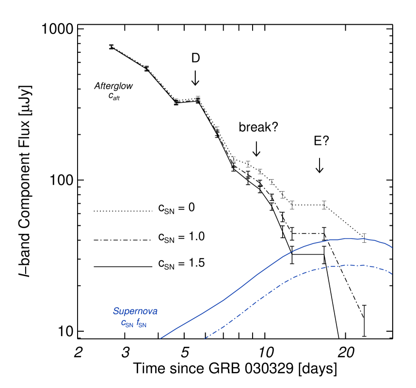
Figure 7: Evolution of the afterglow and supernova brightness at the effective wavelength of the $I$-band filter for different levels of contribution from an underlying supernova. The temporal dependence on the scaling parameter $c_{j,\rm aft}$ is shown as a dotted curve assuming no contribution from a supernovae ($c_{\rm SN}=0$); in Figure 6 we show that a model with $c_{\rm SN}=0$ does not reproduce the color evolution adequately. Instead, a reasonable agreement in both color and flux is obtained by setting $c_{\rm SN}=1.5$. The sum of both components for a given $c_{\rm SN}$ should equal that of the dotted curve within the errors. The fourth re-brightening event (“D” from Granot et al. 2003) is labeled with an arrow at day 5.2. There is some evidence for a break in the light curve between day $\sim$8–10 and another re-brightening event in the light curve around day 15–20, labeled as “E”. The fluxes have been corrected for the effects of dust extinction.

In Figure 7, we show the fit values of $c_{j,\rm aft}$ for three values of $c_{\rm SN}$ as well as the SN model. This analysis demonstrates that the contribution of the SN was $\mathrel{\hbox{\hbox to0.0pt{\hbox{\lower 4.0pt\hbox{$\sim$}}\hss}\hbox{$<$}}}5$% at all the epochs used to derive the extinction in §3.1, and hence the determination of the values for $A_{V}$ and $\beta$ are not strongly affected by the SN. In all cases, the fourth re-brightening event of the afterglow (at $t\approx 5.2$ day; bump “D” in Granot et al. 2003) is clearly seen. With a non-negligible contribution from the SN, the decomposition reveals another steepening around 8–10 days, followed by a possible fifth re-brightening event around 15–20 days. Our favored valued of $c_{\rm SN}=1.5$ implies an equipartition of the afterglow and supernova contribution to the transient light at day $11-13$ in the $I$-band, consistent with the spectral decomposition from Matheson et al. (2003).

4 Discussion and Conclusions

Our analysis of the ANDICAM data has shown that, until day $\sim$5, the transient light is dominated by the afterglow. During the early epochs, the spectrum remains statistically achromatic, even during a re-brightening event. Starting around day 6, the transient slowly evolves in color as the supernova begins to contribute to the total light (Fig. 6 and §3.2). In the optical bandpasses, the early broadband spectrum is consistent with $\beta=-0.94$, reported by Stanek et al. (2003) and Lee et al. (2003) but is more shallow in the IR (Fig. 2). Hjorth et al. (2003) report a significantly more red spectral index of the afterglow component ($\beta=-1.2\pm 0.05$) constrained mostly from their April 3.10 spectrum obtained on the Very Large Telescope (VLT). This is inconsistent with our broadband spectral measurement. One explanation for the discrepancy is that there may have been considerable differential light loss (Filippenko, 1982) in the VLT spectrum: over the course of the three 600 sec exposures, the parallactic angle (East of North) changed from $\approx-170^{\circ}$ to $170^{\circ}$ yet the position angle of the slit was fixed at 123.6^∘, i.e,. more than 40^∘ from the optimal angle. Though the spectroscopic slit width was between 1.3 to 2 times the average seeing, the combination of the high airmass ($\sec z=1.44$) and this chosen slit angle could easily account for the anomalous redness of the Hjorth et al. (2003) spectra.

The measurement of the line–of–sight dust extinction in early GRB afterglows is critical to determine the parameters of the shock physics (e.g., Berger et al., 2001), to provide a means to deredden the flux of any coincident supernova (e.g., Price et al., 2002), and (in conjunction with an $N_{H}$ measurement from X-ray spectroscopy) to constrain the extent of dust destruction near the explosion site (Galama & Wijers, 2001). Our constraint on the line–of–sight extinction toward GRB 030329, $A_{V}$(host) $\leq(0.30\pm 0.03)$ mag is obtained under the assumption that the electron energy index $\beta<-0.5$. Matheson et al. (2003), using independent broadband photometry from $U$–$H$-band on day 5.6, find a consistent value of $A_{V}$(host) = $0.23\pm 0.25$ and $\beta=-0.71\pm 0.21$. As demonstrated in Figure 3, the coupling between the fit values of $A_{V}$(host) and $\beta$ is non-negligible; therefore, we caution that any subsequent use of these measured quantities should take this covariance into account. Specifically, the lowest values of the $\chi^{2}$ surface are well-reproduced under the simple constraint that $\beta=0.92\,A_{V}$(host)$-0.75$ (for $R_{V}$(host) = 3.1). Thus if $A_{V}$(host)$=0$ mag, then $\beta=-0.75$.

We compare the line-of-sight extinction toward GRB 030329 with the average extinction toward Hii regions in the host galaxy. Assuming case-B recombination and the Osterbrock (1974) interstellar extinction curve, the H$\alpha$/H$\beta$ ratio can be converted to $E(B-V)$ using

$$E(B-V)=2.21\log\left(\frac{L_{H\alpha}}{2.76L_{H\beta}}\right).$$ (3)

Using Balmer line luminosities measured by (Hjorth et al., 2003) we find $E(B-V)=-0.01\pm 0.25$. Taking the Galactic extinction of $E(B-V)=0.025$ into account we find $E(B-V)<0.23$, and $A_{V}<0.76$. This is comparable to the extinction inferred by Matheson et al. (2003). We note that the line luminosities have not been corrected for Balmer absorption, as the host luminosity is not yet known; however, since the equivalent widths of the Balmer lines are large when the supernova and afterglow still dominated, this correction will be negligible for H$\alpha$ and H$\beta$. The low extinction in the line–of–sight toward GRB 030329 is therefore typical for star forming regions in this galaxy, and should therefore not be taken as evidence for the destruction of dust by the GRB itself (e.g., Waxman & Draine, 2000).

As shown in Figure 3, a value of $\beta<-0.8$ is formally excluded from the locus of acceptable fits in both cases of $R_{V}$(host). This then excludes any possibility that the synchrotron cooling break moved through the optical/IR bandpass from 2–6 days after the GRB. In the §3.2 we showed that the passage of cooling break could not explain the subsequent color changes from day 6–15, and was therefore also unlikely to have moved through the optical/IR bandpass during that time.

The suggested late-time afterglow features seen in Figure 7 are also an important clue for understanding the structure of GRB explosions. Berger et al. (2003) suggest that the break in the radio light curve around day 10 should have been accompanied by a second break in the optical light curve. Our decomposed afterglow light curve does indeed show some evidence for such a break around day 8–10. The precise timing of the break and the slope of the post-break afterglow light curve depends sensitively on the value of $c_{\rm SN}$. Based on only a few later-time data points, we also suggest tentative evidence for a fifth re-brightening event around day 15–20. If true, the mechanism for the later-time injection of energy into the radiating front must continue at least until this time.

As shown in Figure 6, a concurrent supernova about 50% brighter than SN 1998bw helps to reproduce the reddening in the $B-V$ color and the bluing in the $V-I$ and $V-J$ colors. The supernova plus afterglow model is certainly not a perfect (nor unique) fit to the data, likely due to the inherent uncertainties in modeling the supernova a priori. For instance, the modeled SN over-predicts the late-time flux at epoch 13 by $\approx 0.2-0.3$ mag (this effect was also noted by Hjorth et al. 2003). While the spectroscopy of the SN shows it to be conclusively of type Ic (Hjorth et al., 2003; Chornock et al., 2003; Matheson et al., 2003; Kawabata et al., 2003), there is a large observed diversity in color and light curves from this class of supernovae (e.g., Iwamoto et al., 1998; Mazzali et al., 2002). SN 2003dh could simply have risen and decayed faster than 1998bw (see also Bloom et al. 2002). Instead, the supernova could have occurred a few days before the GRB (the “supranova” scenario; Vietri & Stella 1998; Hjorth et al. 2003). However, as Guetta & Granot (2003) emphasize, had a GRB occurred within a few days (or even a few months) after an SN, the optical depth to Thompson scattering from the SN shell would be much larger than unity, thus extinguishing the GRB. A highly asymmetric SN explosion could produce lower optical depths for certain viewing geometries, but the lack of strong polarization in the SN spectrum suggests a modest level of asymmetry (Kawabata et al., 2003). We therefore conclude that the SN and GRB explosions were contemporaneous to within the free-fall collapse time of the progenitor star (see Guetta & Granot 2003).

Since we did not observe during the peak of the SN (see Figure 1), we do not have a direct measurement of the peak SN brightness. However, assuming a 1998bw-like evolution of the supernova component, scaled to be 1.5 times brighter (0.44 mag), the peak absolute magnitude of 2003dh is $M_{V}=-19.8-5\,\log_{10}h_{65}$ mag; we estimate an uncertainty in this value due to $c_{\rm SN}$ of 0.3 mag. There is an additional $\sim$10% systematic uncertainty in this quantity owing to the unknown peculiar velocity of the host of SN 1998bw.

We end by highlighting one of the unique features of ANDICAM, namely the ability to simultaneously image afterglows in both the optical and infrared bands. Aside from allowing for efficient characterization of the broadband spectrum to measure line–of–sight extinction, any short timescale ($\sim$minutes) color changes in the afterglow could be detected unambiguously. If such observations were to be conducted in the first few hours after a GRB, strong constraints on the passage of the synchrotron peak frequency could be obtained, leading to precision measurements of the peak Lorentz factor of the shell. In addition, the constraints on short term color variations would lead to constraints on the patchiness of clouds near the progenitor (Kumar & Piran, 2000). Indeed, with such instruments in the Swift era we look forward to a level of insight even beyond that gleaned from observations of the remarkable transient of GRB 030329.

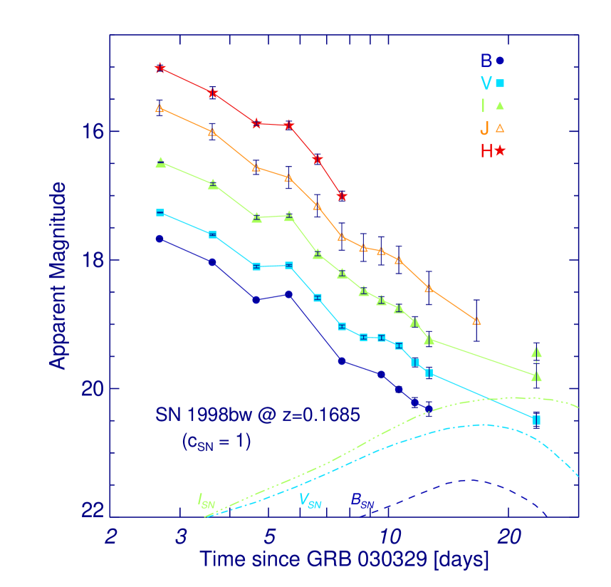
Figure 1: The observed light curve of the transient associated with GRB 030329. The complex bumps and wiggles in the early afterglow, especially the re-brightening event at day $\sim$5.2, are apparent. Shown are the modeled light curves in the BVI filters (dashed, dot-dashed, dash-dotted, respectively) of SN 1998bw at the redshift of GRB 030329 and dimmed by the total line–of–sight extinction inferred for the afterglow (see text). The SN brightness scaling ($c_{\rm SN}$) is later varied in §3.2 to decompose the light curve into an afterglow and SN component.

Figure 4: Best-fit afterglow spectrum plus extinction assuming $\beta=-0.5$ ($p=2$, slow cooling). As in Figure 3, the Galactic extinction is fixed. The dotted line shows the unreddened afterglow spectrum. The dashed line shows the afterglow spectrum reddened only with Galactic extinction. The solid line shows the afterglow after reddening from the Galaxy and a host line–of–sight extinction of $A_{\rm V}=0.30\pm 0.03$ mag (assuming $R_{\rm V}$(host) $=3.1$). This fit is acceptable, with $\chi^{2}$/dof $=0.94$.

Figure 5: Power-law fit to the evolving intrinsic transient spectrum as a function of time, fixing the extinction measured in Fig. 4. The top panel gives the value for $\beta$ and the associated 1 $\sigma$ error assuming an acceptable fit. The bottom panel gives the $\chi^{2}$/dof of the fit. Measurements at epochs marked with solid circles are acceptable fits ($\chi^{2}$/dof $<2$), implying that the transient can be adequately modeled as a single power-law. Open circles show unacceptable fits to a single power-law.

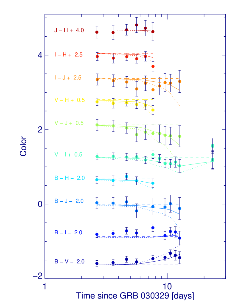
Figure 6: Color evolution of the observed transient compared with a model for the afterglow and the supernova component. The observed data, uncorrected for dust extinction, is shown with 1-$\sigma$ error bars. The model, using a mix of an afterglow and a 1998bw-like supernova, was constructed following §3.2. The dashed horizontal line derives from the best fit result to $c_{j,\rm aft}$ assuming no contribution from a supernova (i.e., $c_{\rm SN}=0$). The solid (dotted) lines show the color results for $c_{\rm SN}=1.5$ (3.0). The $c_{\rm SN}=1.5$ helps reproduce the apparent bluing trend in $V-I$, $V-J$, and $V-H$ and the reddening trend in $B-V$. Such color trends are a natural consequence of an SN source spectrum which peaks around 5000–6000 Å.

Table 1: Photometric Observations of GRB 030329

Date	$\Delta t$	Filter	Exp. Time	Airmass	Mag.	Flux
UT	day		sec	$\sec z$		$\mu$Jy
(1)	(2)	(3)	(4)	(5)	(6)	(7)
Epoch 1, $\delta t=38.5$ min
Apr 1 03:33:29	2.664	B	600.00	1.64	$17.67\pm 0.01$	$341.1\pm 9.9$
Apr 1 03:45:52	2.673	V	600.00	1.67	$17.26\pm 0.01$	$442.8\pm 17.7$
Apr 1 04:01:30	2.684	I	600.00	1.71	$16.48\pm 0.01$	$613.8\pm 31.9$
Apr 1 03:33:27	2.664	J	560.19	1.64	$15.64\pm 0.12$	$863.5\pm 104.1$
Apr 1 03:45:50	2.673	H	560.18	1.67	$15.02\pm 0.05$	$981.2\pm 62.0$
Epoch 2, $\delta t=35.1$ min
Apr 2 02:19:40	3.613	B	600.00	1.62	$18.03\pm 0.01$	$243.9\pm 7.3$
Apr 2 02:31:56	3.621	V	600.00	1.61	$17.61\pm 0.01$	$322.6\pm 13.3$
Apr 2 02:44:17	3.630	I	600.00	1.61	$16.82\pm 0.02$	$449.2\pm 25.0$
Apr 2 02:19:38	3.613	J	560.19	1.62	$16.01\pm 0.13$	$613.6\pm 77.1$
Apr 2 02:31:53	3.621	H	560.18	1.61	$15.40\pm 0.09$	$689.5\pm 68.2$
Epoch 3, $\delta t=34.9$ min
Apr 3 03:21:50	4.656	B	600.00	1.63	$18.62\pm 0.01$	$142.1\pm 4.5$
Apr 3 03:34:01	4.664	V	600.00	1.66	$18.10\pm 0.02$	$204.1\pm 9.0$
Apr 3 03:46:14	4.673	I	600.00	1.69	$17.34\pm 0.03$	$278.7\pm 16.4$
Apr 3 03:21:48	4.656	J	480.15	1.63	$16.56\pm 0.11$	$368.7\pm 41.3$
Apr 3 03:33:58	4.664	H	560.20	1.66	$15.88\pm 0.03$	$443.6\pm 23.4$
Epoch 4, $\delta t=34.9$ min
Apr 4 02:29:21	5.620	B	600.00	1.61	$18.54\pm 0.02$	$153.8\pm 5.5$
Apr 4 02:41:30	5.628	V	600.00	1.61	$18.08\pm 0.01$	$207.7\pm 8.7$
Apr 4 02:53:44	5.636	I	600.00	1.61	$17.31\pm 0.03$	$285.8\pm 16.3$
Apr 4 02:29:18	5.619	J	560.18	1.61	$16.72\pm 0.17$	$318.8\pm 52.3$
Apr 4 02:41:28	5.628	H	560.18	1.61	$15.91\pm 0.07$	$431.9\pm 33.6$
Epoch 5, $\delta t=33.2$ min
Apr 5 02:55:21	6.638	V	600.00	1.61	$18.59\pm 0.03$	$130.6\pm 6.1$
Apr 5 03:07:36	6.646	I	600.00	1.63	$17.90\pm 0.03$	$165.8\pm 9.9$
Apr 5 02:44:50	6.630	J	480.17	1.61	$17.16\pm 0.17$	$212.5\pm 35.4$
Apr 5 02:55:19	6.638	H	560.19	1.61	$16.43\pm 0.08$	$266.0\pm 23.3$
Epoch 6, $\delta t=34.6$ min
Apr 6 02:54:10	7.637	B	600.00	1.62	$19.57\pm 0.02$	$59.2\pm 2.1$
Apr 6 03:06:13	7.645	V	600.00	1.63	$19.03\pm 0.03$	$86.6\pm 4.0$
Apr 6 03:18:20	7.654	I	600.00	1.65	$18.21\pm 0.04$	$125.3\pm 7.9$
Apr 6 02:54:08	7.637	J	560.17	1.62	$17.64\pm 0.21$	$136.7\pm 27.4$
Apr 6 03:06:11	7.645	H	560.21	1.63	$17.01\pm 0.08$	$156.9\pm 13.3$
Epoch 7, $\delta t=34.7$ min
Apr 7 03:30:34	8.662	V	600.00	1.69	$19.20\pm 0.03$	$74.2\pm 3.5$
Apr 7 03:42:45	8.670	I	600.00	1.72	$18.48\pm 0.05$	$97.6\pm 6.6$
Apr 7 03:18:28	8.654	J	560.18	1.66	$17.81\pm 0.22$	$116.9\pm 23.9$
Epoch 8, $\delta t=34.6$ min
Apr 8 01:48:29	9.591	B	600.00	1.63	$19.78\pm 0.03$	$48.9\pm 2.0$
Apr 8 02:12:35	9.608	V	600.00	1.61	$19.21\pm 0.04$	$73.7\pm 3.8$
Apr 8 02:00:33	9.600	I	600.00	1.62	$18.62\pm 0.05$	$85.4\pm 6.1$
Apr 8 01:48:26	9.591	J	1800.18	1.63	$17.86\pm 0.22$	$111.4\pm 23.1$
Epoch 9, $\delta t=34.5$ min
Apr 9 02:21:09	10.614	B	600.00	1.61	$20.01\pm 0.04$	$39.5\pm 2.0$
Apr 9 02:45:13	10.631	V	600.00	1.62	$19.33\pm 0.04$	$65.7\pm 3.4$
Apr 9 02:33:09	10.622	I	600.00	1.61	$18.75\pm 0.06$	$76.2\pm 5.7$
Apr 9 02:25:49	10.617	J	1680.18	1.61	$18.00\pm 0.21$	$98.0\pm 19.7$
Epoch 10, $\delta t=36.4$ min
Apr 10 03:05:21	11.645	B	600.00	1.65	$20.22\pm 0.08$	$32.7\pm 2.5$
Apr 10 03:31:19	11.663	V	600.00	1.72	$19.59\pm 0.07$	$51.8\pm 4.0$
Apr 10 03:17:38	11.653	I	600.00	1.68	$18.96\pm 0.08$	$62.4\pm 5.7$
Epoch 11, $\delta t=36.0$ min
Apr 11 02:47:16	12.632	B	600.00	1.63	$20.32\pm 0.11$	$29.8\pm 3.2$
Apr 11 03:12:50	12.650	V	600.00	1.68	$19.76\pm 0.09$	$44.5\pm 4.0$
Apr 11 03:00:10	12.641	I	600.00	1.65	$19.23\pm 0.12$	$48.8\pm 5.9$
Apr 11 02:47:14	12.632	J	1800.19	1.63	$18.44\pm 0.26$	$65.5\pm 15.9$
Epoch 12, $\delta t=33.4$ min
Apr 15 02:58:11	16.640	J	1920.15	1.68	$18.94\pm 0.32$	$41.1\pm 12.3$
Epoch 13, $\delta t=36.2$ min
Apr 21 23:36:46	23.500	V	450.00	1.90	$20.48\pm 0.11$	$22.9\pm 2.5$
Apr 21 23:46:05	23.506	V	450.00	1.85	$20.50\pm 0.12$	$22.4\pm 2.6$
Apr 21 23:55:43	23.513	I	450.00	1.80	$19.80\pm 0.19$	$28.9\pm 5.3$
Apr 22 00:05:07	23.519	I	450.00	1.76	$19.42\pm 0.14$	$40.8\pm 5.5$

Note. — These photometric observations have been grouped into thirteen epochs. The total duration of the epoch — from the time of the beginning of the first exposure until the ending time of the last exposure — is shown as $\delta t$.

References

- Bailyn et al. (1999) Bailyn, C. D., Depoy, D., Agostinho, R., Mendez, R., Espinoza, J., and Gonzalez, D. 1999, Bulletin of the American Astronomical Society, 31, 1502
- Berger et al. (2001) Berger, E. et al. 2001, ApJ, 556, 556
- Berger et al. (2003) Berger, E. et al. 2003, Nature, in press
- Bessell & Brett (1988) Bessell, M. S. and Brett, J. M. 1988, PASP, 100, 1134
- Blake & Bloom (2003) Blake, C. and Bloom, J. S. 2003, GCN Report 2011
- Bloom (2003) Bloom, J. S. 2003, To be published in the Proceedings of Gamma Ray Bursts in the Afterglow Era, Third Workshop; astro-ph/0303478
- Bloom et al. (1998) Bloom, J. S. et al. 1998, ApJ (Letters), 508, L21
- Bloom et al. (2002) —. 2002, ApJ (Letters), 572, L45
- Burenin et al. (2003) Burenin, R. A., Sunyaev, R. A., Pavlinsky, M. N., et al. 2003, Astronomy Letters, 29, 573
- Burstein (2003) Burstein, D. 2003, submitted; astro-ph/0306591
- Cardelli et al. (1989) Cardelli, J. A., Clayton, G. C., and Mathis, J. S. 1989, ApJ, 345, 245
- Chevalier & Li (1999) Chevalier, R. A. and Li, Z.-Y. 1999, ApJ (Letters), 520, L29
- Chornock et al. (2003) Chornock, R., Foley, R. J., Filippenko, A. V., Papenkova, M., Weisz, D., and Garnavich, P. 2003. IAU Circ. No. 8114
- Dai & Cheng (2001) Dai, Z. G. and Cheng, K. S. 2001, ApJ (Letters), 558, L109
- Filippenko (1982) Filippenko, A. V. 1982, PASP, 94, 715
- Fox et al. (2003) Fox, D. W. et al. 2003, Nature, 422, 284
- Fukugita et al. (1995) Fukugita, M., Shimasaku, K., and Ichikawa, T. 1995, PASP, 107, 945
- Galama et al. (1998) Galama, T. J. et al. 1998, Nature, 395, 670
- Galama & Wijers (2001) Galama, T. J. and Wijers, R. A. M. J. 2001, ApJ (Letters), 549, L209
- Garnavich et al. (2003a) Garnavich, P., Matheson, T., Olszewski, E. W., Harding, P., and Stanek, K. Z. 2003a. IAU Circ. No. 8114
- Garnavich et al. (2003b) Garnavich, P., Stanek, K. Z., and Berlind, P. 2003b, GCN Report 2018
- Granot et al. (2003) Granot, J., Nakar, E., and Piran, T. 2003, submitted; astro-ph/0304563
- Greiner et al. (2003) Greiner, J. et al. 2003, GCN Report 2020
- Guetta & Granot (2003) Guetta, D. and Granot, J. 2003, to appear the Proceedings of ”Gamma Ray Bursts in the Afterglow Era, Third Workshop” (Rome, Sept 2002); astro-ph/0302282
- Henden (2003) Henden, A. 2003, GCN Report 2023
- Henden et al. (2003) Henden, A., Canzian, B., Zeh, A., and Klose, S. 2003, GCN Report 2123
- Hjorth et al. (2003) Hjorth, J. et al. 2003, Nature, 423, 847
- Iwamoto et al. (1998) Iwamoto, K. et al. 1998, Nature, 395, 672
- Kawabata et al. (2003) Kawabata, K. S. et al. 2003, ApJ (Letters), 593, L19
- Kim et al. (1996) Kim, A., Goobar, A., and Perlmutter, S. 1996, PASP, 108, 190
- Kumar & Piran (2000) Kumar, P. and Piran, T. 2000, ApJ, 535, 152
- Lee et al. (2003) Lee, B. C., Lamb, D. Q., Tucker, D. L., and Kent, S. 2003, GCN Report 2096
- Li et al. (2003) Li, W., Chornock, R., Jha, S., and Filippenko, A. V. 2003, GCN Report 2064
- Lipkin et al. (2003a) Lipkin, Y., Ofek, E. O., and Gal-Yam, A. 2003a, GCN Report 2034
- Lipkin et al. (2003b) Lipkin, Y., Ofek, E. O., Gal-Yam, A., Leibowitz, E. M., and Mendelson, M. 2003b, GCN Report 2045
- Lipkin et al. (2003c) Lipkin, Y. M., Ofek, E. O., Gal-Yam, A., et al. 2003c, in prep
- Matheson et al. (2003) Matheson, T. et al. 2003, accepted to ApJ; astro-ph/0307435
- Mazzali et al. (2002) Mazzali, P. A. et al. 2002, ApJ (Letters), 572, L61
- Osterbrock (1974) Osterbrock, D. E. 1974, Astrophysics of gaseous nebulae (San Francisco: W. H. Freeman and Co.)
- Patat et al. (2001) Patat, F. et al. 2001, ApJ, 555, 900
- Persson et al. (1998) Persson, S. E., Murphy, D. C., Krzeminski, W., Roth, M., and Rieke, M. J. 1998, AJ, 116, 2475
- Peterson & Price (2003) Peterson, B. A. and Price, P. A. 2003, GCN Report 1985
- Price et al. (2003a) Price, A. et al. 2003a, GCN Report 2156
- Price et al. (2002) Price, P. A. et al. 2002, ApJ (Letters), 572, L51
- Price et al. (2003b) —. 2003b, Nature, 423, 844
- Rhoads (1997) Rhoads, J. E. 1997, ApJ (Letters), 487, L1
- Rykoff & Smith (2003) Rykoff, E. S. and Smith, D. A. 2003, GCN Report 1995
- Sari et al. (1998) Sari, R., Piran, T., and Narayan, R. 1998, ApJ (Letters), 497, L17
- Sato et al. (2003) Sato, R., Yatsu, Y., Suzuki, M., and Kawai, N. 2003, GCN Report 2080
- Schlegel et al. (1998) Schlegel, D. J., Finkbeiner, D. P., and Davis, M. 1998, ApJ, 500, 525
- Stanek et al. (2003) Stanek, K. Z. et al. 2003, ApJ (Letters), 591, L17
- Tiengo et al. (2003) Tiengo, A., Mereghetti, S., Ghisellini, G., Rossi, E., Ghirlanda, G., and Schartel, N. 2003, submitted to A&A; astro-ph/0305564
- Torii (2003) Torii, K. 2003, GCN Report 1986
- Uemura et al. (2003) Uemura, M. et al. 2003, Nature, 423, 843
- van Dokkum (2001) van Dokkum, P. G. 2001, PASP, 113, 1420
- Vanderspek et al. (2003) Vanderspek, R. et al. 2003, GCN Report 1997
- Vietri & Stella (1998) Vietri, M. and Stella, L. 1998, ApJ (Letters), 507, L45
- Waxman & Draine (2000) Waxman, E. and Draine, B. T. 2000, ApJ, 537, 796
- Wood-Vasey et al. (2003) Wood-Vasey, W. M., Nugent, P., Lee, B. C., Bambery, R., Pravdo, S., Hicks, M., and Lawrence, K. 2003, GCN Report 1998
- Woosley et al. (1999) Woosley, S. E., Eastman, R. G., and Schmidt, B. P. 1999, ApJ, 516, 788