Observations of cluster substructure using weakly lensed sextupole moments

Abstract

Since dark matter clusters and groups may have substructure, we have examined the sextupole content of Hubble images looking for a curvature signature in background galaxies that would arise from galaxy-galaxy lensing. We describe techniques for extracting and analyzing sextupole and higher weakly lensed moments. Indications of substructure, via spatial clumping of curved background galaxies, were observed in the image of CL0024 and then surprisingly in both Hubble deep fields. We estimate the dark cluster masses in the deep field. Alternatives to a lensing hypothesis appear improbable, but better statistics will be required to exclude them conclusively. Observation of sextupole moments would then provide a means to measure dark matter structure on smaller length scales than heretofore.

I Introduction

The observations of the Supernova Cosmology Project and the High-z Supernova Search team supernova ; Riess:1998cb ; Tonry:2003zg as well as the Cosmic Microwave Background observation Bond , later confirmed by the Wilkinson Microwave Anisotropy Probe (WMAP) Spergel:2003cb , suggest the possibility of an accelerating expansion of the Universe, which could mean the presence of a positive cosmological constant or dark energy. These observations give rise to questions as to the nature of this dark energy/cosmological constant, possible predictions for the evolution of the Universe based on this assumption, and possible ways to improve or find new observational methods that could lead to a better understanding of this evolution.

Weak gravitational lensing methods (for review see Bartelmann:1999yn ; Mellier:1998pk ; Hoekstra:2002nf and references therein), that allow one to investigate the evolution of matter clustering and the growth of large-scale structure Wittman:2000tc ; Mellier:2002vp , are a way to probe both dark energy and dark matter. In a sense it is a unique way to investigate both the past and future of the universe. The large structure growth is defined by the growth of the matter density fluctuations predicted by inflationary cosmology and dark energy evolution (for review see Peebles:xt ). The structure of density fluctuations provides information about inflationary scenarios Huterer:2000mj ; Huterer:2001yu ; Linder:2003dr . On the other hand, the matter distribution measurements give bounds on the dark energy equation of state, allowing one to predict the future of the universe Linde:2002gj ; Kallosh:2003mt ; Kallosh:2003bq .

The traditional weak gravitational lensing techniques Kaiser:2000if , despite observational superiority in measuring the large clumps of matter such as clusters of galaxies (visible or dark) with $10^{14}\,M_{\odot}$ are not sensitive to the substructure of such clusters or smaller groups and clumps of matter. We have investigated a possibility to use more sensitive methods to expose such substructure and detect the presence of smaller clumps. The development of these methods and their application to analysis of data from the future observational projects like the SuperNova /Acceleration Probe (SNAP) unknown:2002dp ; SNAP , and the Large Synoptic Survey Telescope (LSST) Tyson:2003kb promise to expand our knowledge of large scale structure to scales unreachable by other techniques such as microwave background anisotropy or traditional weak lensing. These observations could make an important contribution to the understanding of dark matter structure as well as possible inflationary scenarios.

Arclets are a familiar strong-lensing phenomena Bartelmann:1999yn ; Mellier:1998pk . They are an example of the general property that the nonlinear 1/r deflections of a light stream passing a mass concentration will produce, relative to the stream centroid, a full complement of moments. The curving seen in the arclet can be understood as the correlated superposition of a quadrupole and sextupole moment, with the length of the arclet usually determined by the strength of the octupole moment.

To date, weak lensing has concentrated exclusively on quadrupole moments - ellipticity Kaiser:2000if , because usually all other lensing-induced higher moments are smaller than the lensing-induced quadrupole moments (that are already small compared to background galaxy ellipticities). A typical measurable cluster has a mass of 10¹⁴ solar masses and a radius of 500 kpc. Since the strength of the quadrupole kick is proportional to the mass and falls off like 1/r², one could get the same quadrupole moment in a light stream positioned 5 kpc from an object of 10¹⁰ solar masses. In the latter example, since the sextupole moment varies as 1/r³, the sextupole moment becomes 100 times stronger, becoming larger than the intrinsic sextupole moments of background galaxies. It occurred to us that if clusters or groups contain an abundance of lower mass clumps, the light streams passing through these groups might occasionally pass close to a small mass clump producing an observable sextupole moment in the image finalfocus . In this case one can expect a correlation between the direction of the quadrupole and sextupole moments.

To investigate this hypothesis we considered the images of the North and South Hubble Deep Fields (HDF) Williams:1996ay ; Casertano:2000wy as well as some other Hubble images of known clusters, such as CL0024. We used SExtractor software sextractor to select either faint images (typically 23$<$m$<$29 ) or used z-catalogs (when available) to identify distant galaxies with z$>$0.7.

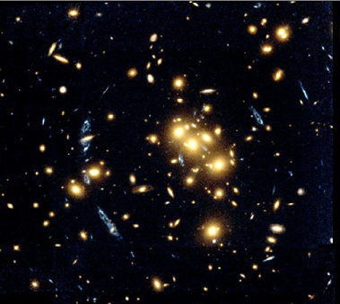
Figure 1: Hubble image of galaxy cluster CL0024.

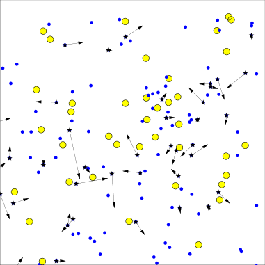
Figure 2: m-selected background galaxies of the cluster CL0024 are indicated by blue dots and foreground galaxies by yellow circles. The small stars with arrows indicate the “curved” background galaxies with the arrow pointing toward the scattering center and its length proportional to the strength of the quadrupole moment.

The “curved” galaxies we sought were identified as those whose sextupole moment was oriented so that one of its minima was aligned within a few degrees of a quadrupole minimum. We will refer to galaxies which have a quadrupole maximum aligned with a sextupole maximum as “ aligned ” galaxies.

Figures 1 and 2 show the CL0024 cluster and the location of the background galaxy sample and its “curved” members. The arrows point in the direction of the scattering center and their length is proportional to the strength of the quadrupole moments. There is clear evidence of clumping toward the center of this cluster. To our surprise, “curved” galaxies were also clumped in both the north and south fields of the HDF survey. The probability for the observed clumping to occur by chance was about $1\%$ for each field.

We have carried out other tests that support the hypothesis that the observed clumping comes from lensing: 1) “aligned” galaxies were predicted and found to be clumped as strongly as curved galaxies, 2) galaxies halfway between “aligned” and ”curved” were predicted and found to have no clumping, 3)“curved” galaxies were predicted and found to have smaller moments than all galaxies, and 4) “aligned” galaxies were predicted and found to have moment strengths distributed as all other background galaxies.

We have considered causes other than lensing for the spatial clumping of curved galaxies, such as instrumental effects, computational effects, or other physical phenomena. For example, since the background galaxies are known to be clumped, our result could be the consequence of the fact that, for some unknown reason, galaxies in some groups tend to be more curved than in other groups. Or perhaps galaxies of a certain epoch tend to be more curved. The tests we have constructed and their implications for each alternative hypothesis are discussed and the results summarized in Table I.

Finally, assuming we are indeed seeing lensing, we have made an initial attempt to deduce the mass of the objects doing the lensing and the mass of the group in which they reside. The mass of the group is easier to estimate than the mass of the lensing objects themselves, in that the former depends only on the i) the size of the observed group, ii) the fraction of background galaxies that are lensed, and iii) the average induced quadrupole moment. The results we present here are preliminary.

Since in some cases the footprint of the observed galaxy could pass through a dark matter clump, we present an approach to this general situation as well. While individual mass measurements remain out of reach, it could be expected that modeling would supply a basis to deduce well-defined statistical results when analyzing larger pieces of sky.

II Theoretical framework

Fig.4 shows rays from a distant background galaxy being deflected by a mass concentration. The apparent image, as seen by the telescope, is defined by an intensity function which depends only on the angle of each ray as it enters the telescope. Following a ray backwards, toward the apparent image, it is deflected by mass distributions, but is known to depart somewhere from the source galaxy. It will have a definite position and angle at the source galaxy (measured relative to the position and angle of the centroid ray). This map from telescope variables to source variables will be symplectic since the light geodesics are described by a Hamiltonian. From the point of view of the galaxy, all rays traced backward from the telescope come from the same point. Hence the two angles at the telescope uniquely describe the trajectory through space and the initial position $x_{S}$ and $y_{S}$ (and angle ${x}^{\prime}_{S}$ and ${y}^{\prime}_{S}$) at the galaxy. So the “backwards” map can be written as a set of 4 functions $x_{S}(x_{T},y_{T}),\;y_{S}(x_{T},y_{T}),\;{x}^{\prime}_{S}(x_{T},y_{T}),\;\mbox{and }{y}^{\prime}_{S}(x_{T},y_{T})$, where “T” designates “telescope” and “S” designates “source”. The coordinate system for both the source and telescope images can be taken to be the pixel grid on the focal plane. The position of the centroid trajectory is taken to be the origin for both images, i.e. the dipole kick suffered by the image as a whole is ignored. Only under special circumstances, such as Einstein rings or point-to-point focusing, will a ray leaving the telescope at two different angles arrive at the same point on the source galaxy. We will not need to consider such cases and hence will be able to drop the two functions ${x}^{\prime}_{S}\mbox{ and }{y}^{\prime}_{S}$. We will be able to assume that the determinant

$$\left|{{\begin{array}[]{*{20}c}{\frac{\partial x_{S}}{\partial x_{T}}\hfill}&{\frac{\partial x_{S}}{\partial y_{T}}\hfill}\\ {\frac{\partial y_{S}}{\partial x_{T}}\hfill}&{\frac{\partial y_{S}}{\partial y_{T}}\hfill}\\ \end{array}}}\right|\neq 0.$$ (1)

The two functions $x_{S}(x_{T},y_{T})\mbox{ and}\;y_{S}(x_{T},y_{T})$ can be combined into one complex function by defining $w_{S}=x_{S}+iy_{S}$. This complex function can be written in terms of the variables $w_{T}=x_{T}+iy_{T}$ and $\bar{w}_{T}=x_{T}-iy_{T}$ by substituting $x_{T}=\frac{1}{2}\left({w_{T}+\bar{w}_{T}}\right)$ and $y_{T}=\frac{1}{2i}\left({w_{T}-\bar{w}_{T}}\right)$. The map equations can then be written as the single function $w_{S}(w_{T,}\bar{w}_{T}).$ Since the transverse width of the light stream will be small compared to characteristic dimensions of the variations of the mass distributions, we may expand this function in a power series about the stream centroid:

$$w_{S}(w_{T},\bar{w}_{T})=w_{T}+\sum\limits_{n,m=0}^{\infty}{a_{nm}w_{T}^{n}}\bar{w}_{T}^{m}.$$ (2)

The $1+a_{10}$ combination of terms is a rotation and scaling, the $a_{01}$ term is a quadrupolar distortion, the $a_{02}$ term is a sextupolar distortion, the $a_{03}$ term is an octupolar distortion, the $a_{20}$ term is a cardioid-like distortion, and the $a_{11}$ term is an $r^{2}$-dependent translation of circles, and so on. We will be concerned with the terms $a_{01}$, $a_{02}$, $a_{03}$, and $a_{20}$ and refer to them more simply by the letters, $a,\;\tilde{b},\;\tilde{c},\mbox{ and }\tilde{\bar{d}}$ respectively. We have introduced the tilde symbol “$\sim$” to alert the reader to the fact that these coefficients have dimensions, and to distinguish them from dimensionless partners we will introduce later. For a map arising from a single kick $a_{01}$ is necessarily real and $a_{11}=2\bar{a}_{20}=2\tilde{d}.$

Since the largest mass distribution size ($\sim$500 kpc) is still small compared to typical path lengths ($\sim$1000 Mpc), and since the light-deflection angles are small ($<$ 10^-4 radians) and can be calculated by multiplying the deflection angles of a non-relativistic particle by 2, one can integrate the transverse component of the 1/r² force from a point distribution along a straight path to get the deflection angle

$$\Delta{r}^{\prime}=-\frac{4MG}{r}=-\frac{4MG}{r_{0}}\left(\frac{1}{1+\frac{r-r_{0}}{r_{0}}}\right)$$

$$\sim \frac{4MG}{r_{0}}\left(-1+\frac{\delta r}{r_{0}}-\left(\frac{\delta r}{r_{0}}\right)^{2}+\left(\frac{\delta r}{r_{0}}\right)^{3}-\cdots\right),$$

where $\delta r=r-r_{0}.$

The potential for this kick is $2\Phi_{\delta}=4MG\,Ln\left[r\right]$, which is the Green’s function for the 2 dimensional Laplace equation, $\nabla^{2}\Phi=4\pi G\rho$, where $\rho$ is the 2D (longitudinally-integrated) density function for the mass distribution.

The usefulness of the complex variables originates in part from the fact that the solution to Laplace’s equation in empty space can be written as the real part of an analytic function. For the point mass source (which would be the same as outside a symmetrical distribution) one may write $2\Phi_{\delta}=4MG\;\,\Re\left(\,Ln\left[{x+iy}\right]\right)$. Expanding about the centroid ray located at some $w_{0}=x_{0}+iy_{0}$ results in (a constant is dropped)

$$2\Phi_{\delta}=-4MG\;\;\Re\left[\,\sum\limits_{n=1}{\frac{1}{n}\left({-\frac{\omega}{\omega_{0}}}\right)}^{n}\right].$$ (4)

It is useful to introduce derivative operators $\frac{\partial}{\partial w}\equiv\frac{1}{2}\left[{\frac{\partial}{\partial x}-i\frac{\partial}{\partial y}}\right]\mbox{ and }\frac{\partial}{\partial\bar{w}}\equiv\frac{1}{2}\left[{\frac{\partial}{\partial x}+i\frac{\partial}{\partial y}}\right]$, which have the property that $\frac{\partial w}{\partial w}=\frac{\partial\bar{w}}{\partial\bar{w}}=1$ and $\frac{\partial\bar{w}}{\partial w}=\frac{\partial w}{\partial\bar{w}}=0$. In terms of these operators the kick from the potential can be written as (the constant dipole kick is dropped)

$$\Delta{w}^{\prime}_{\delta}=-2\frac{\partial\left({2\Phi_{\delta}}\right)}{\partial\bar{w}}=-\frac{4MG}{\bar{w}_{0}}\;\,\sum\limits_{n=2}{\left({-\frac{\bar{w}}{\bar{w}_{0}}}\right)}^{n-1}.$$ (5)

The first three terms of this expression are the quadrupole, sextupole and octupole, respectively (see Fig.4).

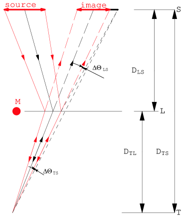
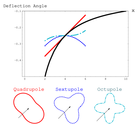
Figure 3: A diagram showing 3 light rays from a source image scattered by a single concentrated mass. The relationship $D_{TS}\Delta\theta_{TS}=D_{LS}\Delta\theta_{LS}$ expresses the observed displacement angle in terms of the deflected angle. Note that the image in the radial direction is narrower than the source width.

Figure 4: The curved line in this graph shows the 1/r kick from a point source. At a point $r_{0}$ this curve may be expanded in a power series (see eq. II) yielding linear, quadratic and cubic terms that are shown by a tangent line, a dashed curve and a dot-dash curve, respectively. The deformation of a constant intensity circle in a light beam centered at $r_{0}$ by each of these terms is also shown here. The straight lines indicate the radial direction from the origin to the center of the light beam. The orientation of these images is such that there is always a deflection minimum toward the scattering center. The quadrupole plus sextupole yields a slight “banana” shape with the radius of curvature originating at the scattering center.

The geometry of Fig.4 shows that $\Delta w_{S}=D_{LS}\;\Delta{w}^{\prime}(w,\bar{w})$, where $D_{LS}$ is the angular-diameter distance between the source and the lens. And if one wishes to obtain the map as a function of the telescope variables rather than the lensing plane variables one may substitute$\mbox{ }w=\frac{D_{TL}}{D_{TS}}w_{T}$.

It follows that the coefficients $a,\;\tilde{b},\;\mbox{and }\tilde{c}$ of this point-source map are given by

$$a_{\delta} = D_{LS}\frac{D_{TL}}{D_{TS}}\frac{4MG}{\bar{w}_{0}^{2}},$$ (6)

$$\tilde{b}_{\delta} = -D_{LS}\left({\frac{D_{TL}}{D_{TS}}}\right)^{2}\frac{4MG}{\bar{w}_{0}^{3}},$$ (7)

$$\tilde{c}_{\delta} = D_{LS}\left({\frac{D_{TL}}{D_{TS}}}\right)^{3}\frac{4MG}{\bar{w}_{0}^{4}}.$$ (8)

The magnitudes of interest will be the rms value of the dimensionless quantities $a_{\delta},\;b=\tilde{b}_{\delta}\sigma,\mbox{ and }c=\tilde{c}_{\delta}\sigma^{2}$, where $\sigma$ is the rms size of the image. Each of these coefficients decreases in magnitude from the previous by $r_{G}/r_{0}$, where $r_{G}\equiv\frac{D_{TL}}{D_{TS}}\sigma$ is the footprint radius of the background galaxy at the lensing mass plane and $r_{0}$ is the distance from the center of the footprint to the center of the lensing mass.

For a potential derived from a solution of Laplace’s equation for a general mass distribution, one can expand the potential about the centroid ray to get its local power series expression. The map obtained from the derivative of this power series potential will necessarily be of the form of equation (2). Since the potential is a real function, its expansion in terms of $w$ and $\bar{w}$ will have some constraints:

1. the coefficients of the linear $w$ and $\bar{w}$ terms must be the complex conjugate of one another, so there is one complex parameter, which is the magnitude and direction of the dipole kick;

2. the coefficients of the $w^{2}$and $\bar{w}^{2}$ must be the complex conjugate of one another, and represent the magnitude and orientation of the quadrupole kick;

3. the coefficient of $w\bar{w}$ must be real (the coefficient of this term must be proportional to $\left.{\frac{\partial}{\partial w}\frac{\partial}{\partial\bar{w}}\Phi}\right|_{0}=\frac{1}{4}\left.{\nabla^{2}\Phi}\right|_{0}=\pi G\left.\rho\right|_{0}$ and hence is zero except when the light path passes through a distribution ) and represents a magnification;

4. the coefficients of the $w^{3}$ and $\bar{w}^{3}$ must be the complex conjugate of one another, and represent the magnitude and orientation of the sextupole kick,

5. the coefficients of the $w^{2}\bar{w}$ and $w\bar{w}^{2}$ must be the complex conjugate of one another, and represent the magnitude and orientation a third order term which is also necessarily zero except when the light path passes through a distribution. In this last case, the kick can be written in the form $\Delta w=\bar{\tilde{d}}{\kern 1.0pt}w_{T}^{2}+2\tilde{d}{\kern 1.0pt}w_{T}\bar{w_{T}}$. $\tilde{d}$ will be proportional to the first derivatives of $\rho$, in fact

   $$\tilde{d}=-2\pi G\,D_{LS}\left(\frac{D_{TL}}{D_{TS}}\right)^{2}\left.{\frac{\partial\rho}{\partial\bar{w}}}\right|_{0}.$$

The final element we will need in a minimum theoretical framework is a method to deduce the coefficients of the map from the image. This process begins by noting the surface brightness relationship $i_{S}(x_{S},y_{S})\,dx_{S}dy_{S}=i_{T}(x_{T},y_{T})\,dx_{T}dy_{T}$, expressing the fact that if the area element is transformed according to the map, the number of photons leaving the source in that area will be the number observed in the image. Defining the (unknown) moments of the source through $M_{nm}^{S}\equiv\int{w_{S}^{n}}\bar{w}_{S}^{m}\,i_{S}(x_{S},y_{S})dx_{S}dy_{S}$, and transforming to telescope variables yields

$$M_{nm}^{S}=$$ (9)

$$\int{w_{S}^{n}(w_{T},\bar{w}_{T})}\bar{w}_{S}^{m}(w_{T},\bar{w}_{T})i_{T}(x_{T},y_{T})dx_{T}dy_{T}.$$

This equation can be used to determine an expression for the quadrupole map coefficient:

$$\begin{array}[]{c}M_{20}^{S}=\int{\left({w_{T}+a\bar{w}_{T}}\right)^{2}\,}i_{T}(x_{T},y_{T})dx_{T}dy_{T}\\ \\ =M_{20}^{T}+2aM_{11}^{T}+a^{2}M_{02}^{T}.\end{array}$$

The moments on the right hand side of this equation can be deduced from the telescope image. One obtains a quadratic equation for $a$: one can assume $M_{20}^{S}=0,$ or one can find a statistical ensemble for $a$ in terms of an assumed statistical ensemble for $M_{20}^{S}$. Note that $w\bar{w}=r^{2}\mbox{ so }M_{11}^{T}$ is the mean square radius of the telescope image. We normalize surface brightness functions so that $\int{i_{T}(x_{T},y_{T})\,dx_{T}dy_{T}=1}$.

Solving for $a$,

$$a=-\frac{\Delta M_{20}}{2M_{11}^{T}}-a^{2}\frac{\bar{M}_{20}^{T}}{2M_{11}^{T}},$$ (10)

where we introduced the notation:

$$\Delta M_{nm}=M_{nm}^{T}-M_{nm}^{S}.$$

Since $\left[{\bar{M}_{20}^{T}/2M_{11}^{T}}\right]_{rms}\approx 0.15$, the last term in (10) is typically only a 2% correction. Though equation (II) may be solved exactly to get

$$a=-\frac{\Delta M_{20}}{2M_{11}^{T}}\frac{2}{1+\sqrt{1-\frac{\Delta M_{20}}{M_{11}^{T}}\frac{\bar{M}_{20}^{T}}{M_{11}^{T}}}}\quad,$$ (11)

we will be content to approximate the 2^nd factor by unity.

To obtain an equation for the sextupole moment consider

$$\begin{array}[]{c}M_{30}^{S}=\int{\left({w_{T}+a\bar{w}_{T}+\tilde{b}\bar{w}_{T}^{2}}\right)^{3}\,}\,i_{T}(x_{T},y_{T})dx_{T}dy_{T}\\ =M_{30}^{T}+3\tilde{b}\,M_{22}^{T}+3a\,M_{21}^{T}+\ldots\\ \end{array}\quad.$$ (12)

whence

$$\tilde{b}\,\approx-\frac{\Delta M_{30}}{3M_{22}^{T}}-\frac{a\,M_{21}^{T}}{M_{22}^{T}}\quad.$$ (13)

Using equation (10) for $a$ and introducing the rms radius of the galaxy to obtain a dimensionless quantity we have

$$b\equiv\tilde{b}\sigma\,\approx\left[{-\Delta M_{30}+\frac{3}{2}\frac{\Delta M_{20}}{M_{11}^{T}}M_{21}^{T}}\right]\frac{\sqrt{M_{11}^{T}}}{3M_{22}^{T}}.$$ (14)

where $\sigma=\sqrt{M_{11}^{T}}$. Here we note the interesting fact that even with $b=0$ the quadrupole term in the map can induce a change in the sextupole moment $\Delta M_{30}$ if $M_{21}^{T}\neq 0$.

An $M_{21}^{T}$ could originate in the background galaxy or be generated by the 3^rd order kick proportional to the derivative of $\rho.$ To examine the latter possibility we look at

$$M_{21}^{S}=\int{\left({w_{T}+\Delta w}\right)^{2}\left({\bar{w}_{T}+\Delta\bar{w}}\right)\,}\,i_{T}(x_{T},y_{T})dx_{T}dy_{T},$$

with $\Delta w=a\bar{w}_{T}+\tilde{b}\bar{w}_{T}^{2}+2\tilde{d}{\kern 1.0pt}w_{T}\bar{w}_{T}+\bar{\tilde{d}}{\kern 1.0pt}w_{T}^{2}$. The result is the equation

$$M_{21}^{S}=M_{21}^{T}+2a\bar{M}_{21}^{T}+\bar{a}M_{30}^{T}+5\tilde{d}M_{22}^{T}+\ldots$$ (15)

$$d = \tilde{d}\sigma$$

$$\approx \left[{-\Delta M_{21}+\frac{\Delta M_{20}}{M_{11}^{T}}\bar{M}_{21}^{T}}+\frac{\bar{\Delta M_{20}}}{2M_{11}^{T}}{M}_{30}^{T}\right]\frac{\sqrt{M_{11}^{T}}}{5M_{22}^{T}},$$

$\tilde{d}$ has the direction opposite to the density gradient and in typical cases would be expected to be along the axis of the minima of the induced quadrupole moment.

Finally, since the telescope image has been blurred by the point-spread function, one needs to know the moments of the point-spread function, and if possible correct its systematic effects on the properties of the measured image. If the complete (no thresholding) image was available one could compute (“^” indicates convolved with the PSF, and $\Delta x_{T}\equiv x_{T}-{x}^{\prime}_{T}$ etc.)

$$\hat{M}_{nm}^{T} = \int{w_{T}^{n}\bar{w}_{T}^{m}\,\hat{i}_{T}(x_{T},y_{T})dx_{T}dy_{T}}$$

$$= \int{\int{w_{T}^{n}\bar{w}_{T}^{m}\,p(\vec{r}_{T}-\vec{{r}^{\prime}}_{T})\,i_{T}({\vec{r}}^{\prime}_{T})dx_{T}dy_{T}d{x}^{\prime}_{T}d{y}^{\prime}_{T}}}$$

$$= \int{\int{\left({\Delta w_{T}+{w}^{\prime}_{T}}\right)^{n}\left({\Delta\bar{w}_{T}+\bar{{w}^{\prime}}_{T}}\right)^{m}\times}}$$

$$\quad\quad p(\Delta\vec{r}_{T})i_{T}({\vec{r}}^{\prime}_{T})d\Delta x_{T}d\Delta y_{T}d{x}^{\prime}_{T}d{y}^{\prime}_{T}.$$

When the binomial powers are expanded, the double integral reduces to the sum of a product of single integrals. One finds, for example,

$$\hat{M}_{20}^{T}=M_{20}^{P}+2M_{10}^{P}M_{10}^{T}+M_{20}^{T}=M_{20}^{P}+M_{20}^{T}.$$ (18)

The left hand side can be determined directly. The first term on the right hand side is the quadrupole moment of the point-spread function, which can be determined presumably by looking at star images. The dipole terms in the central product are both zero by definition of the centroid. The last term is the sought after quadrupole moment of the pure image. Note that if the point-spread function has no quadrupole term the blurred image has the same quadrupole moment as the original image. However the map coefficient $a$ also involves the moment $M_{11}^{T}$, which is different:

$$\hat{M}_{11}^{T} = M_{11}^{P}+M_{10}^{P}M_{01}^{T}+M_{01}^{P}M_{10}^{T}+M_{11}^{T}$$

$$= M_{11}^{P}+M_{11}^{T}.$$

This is a statement that the rms of the final image is equal to the rms of the original image plus the rms of the point-spread function. For completeness, for remaining moments of interest we have

$$\hat{M}_{30}^{T} = M_{30}^{T}+M_{30}^{P},$$ (20)

$$\hat{M}_{21}^{T} = M_{21}^{T}+M_{21}^{P},$$ (21)

and

$$\hat{M}_{22}^{T} = M_{22}^{T}+2M_{11}^{P}M_{11}^{T}+M_{22}^{P}+M_{20}^{P}M_{02}^{T}+M_{02}^{P}M_{20}^{T}$$ (22)

$$\approx M_{22}^{T}+2M_{11}^{P}M_{11}^{T}+M_{22}^{P}.$$

In all cases, if the moments of the point-spread-function are known, the moments of the original image can be found from the smeared image. However this result does not strictly hold when the image is taken to be only those pixels whose count number exceeds some threshold. We will not discuss this problem further here.

III Galaxy selection

The software SExtractor was used to select galaxies from the Hubble deep field and to specify which pixels to include in the image. Galaxy images were transferred to the Mathematica programming environment (see Fig. 5). Galaxies with more than one maxima were eliminated.

  

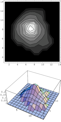
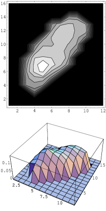
Figure 5: Two galaxy images (contour plots and 3-D plots of surface brightness from the Hubble north field).

Two SExtractor input parameters proved to be significant: i) the threshold setting, which we typically took to be 10 times the noise floor, and ii) the convolution matrix for pixel selection, which we typically took to be 3x3 or a delta function. If the convolution matrix was too broad (larger than 3x3 pixels), important pixels were dropped resulting in a change in the computed moments. That the dropped pixels were important was deduced from the fact that the clumping result described below becoms less significant.

The high threshold is important to observe clumping. In fact the clumping result become less apparent below $5\,\sigma$. Visual examination of galaxy images reveals that at lower thresholds the edges are indeed less crisp, and because the sextupole moment is weighted by $r^{3}$, this moment can be dominated by edge effects.

Setting the threshold at $10\,\sigma$ noise floor results in images which are galaxy cores. About half of all faint galaxies are lost in this cut. Since some fainter galaxies also have “crisp” cores, there may be ways to recover those by imposing a threshold that scales with core brightness.

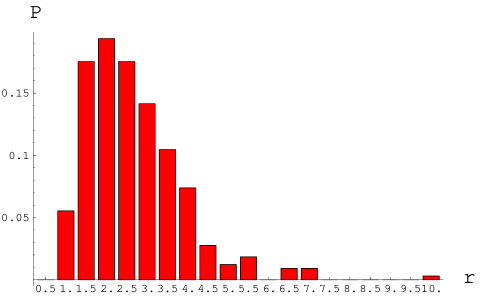
Figure 6: Distribution of galaxy rms core sizes.

Our galaxy-core images have a small rms radius of about 2 pixels. The distribution of rms radii is shown in Fig. 6. The distance across the image is typically 5 pixels. For comparison the rms PSF radius for the Hubble deep field is 1.7 pixels. However for high thresholds the point-spread-function spreads the image less than indicated by its rms radius.

IV Map coefficient strengths

We have carried out studies for galaxies that have been selected by magnitude or by z-value . Results for all quantities were similar. Fig. 7 shows the measured distribution of the quadrupole $a$ coefficient for magnitude-selected north field galaxies with

$$\hat{a}_{0}\equiv-\frac{M_{20}^{T}}{2\hat{M}_{11}^{T}},$$ (23)

($M_{20}^{S}$ is assumed to be zero, “ $\hat{}$ ” indicates smeared quantities are used). The $x$ and $y$ components of the coefficient are well fit by a Gaussian distribution with $\hat{\sigma}_{a0}$= 0.14. The distribution for the magnitude of $a$ is the product of two Gaussians integrated over angle (a Rayleigh distribution) characterized by the same $\hat{\sigma}_{a0}.$ The quadrupole moments of selected galaxies were also calculated using a “weighting-function” technique. The two methods give similar results for the $a$ coefficient.

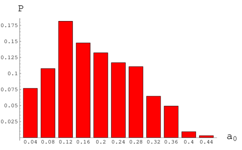
Figure 7: Distribution of the dimensionless quadrupole moment coefficient, $|a_{0}|$.

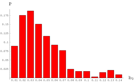
Figure 8: Distribution of the dimensionless sextupole moment coefficient, $|b_{0}|$.

Fig. 8 shows the measured distribution of the dimensionless sextupole coefficient

$$\hat{b}_{0}\equiv-\frac{M_{30}^{T}}{3\hat{M}_{22}^{T}}\sqrt{\hat{M}_{11}^{T}},$$ (24)

($M_{30}^{S}$ is assumed to be zero, the $\Delta M_{20}^{T}$ term is ignored) for m-selected galaxies in the north field. The $x$ and $y$ component of the coefficient is again Gaussian with $\hat{\sigma}_{b0}$=0.034 being a factor of 4 smaller than the quadrupole moment $\hat{\sigma}_{a0}$. Fig. 9 shows the measured distribution for the sextupole-order $d$ coefficient

$$\hat{d}_{0}\equiv-\frac{M_{21}^{T}}{5\hat{M}_{22}^{T}}\sqrt{\hat{M}_{11}^{T}},$$ (25)

( $M_{21}^{S}$ is assumed to be zero and the $\Delta M_{30}\mbox{ and }\Delta M_{20}$ terms are ignored ) for m-selected galaxies in the north field. The $x$ and $y$ component of the coefficient are again Gaussian. $\hat{\sigma}_{d0}$=0.009, is a factor of more than 15 smaller than the quadrupole moment $\hat{\sigma}_{a0}$ and about a factor of 4 smaller than $\hat{\sigma}_{b0}.$ Referring to equation (14) we see that the magnitude of the 2^nd correction term can be estimated to be typically a factor of 10 smaller than the leading term. In equation (II) we can estimate that the 2^nd and 3^rd term are typically a factor of 3 smaller than the leading term.

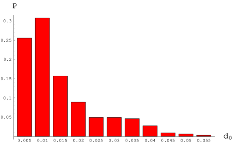
Figure 9: Distribution of the dimensionless coefficient $|d_{0}|$.

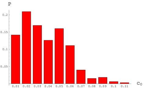
Figure 10: Distribution of the dimensionless octupole moment coefficient, $|c_{0}|$.

Finally, Fig. 10 shows the distribution of the dimensionless octupole coefficient

$$\hat{c}_{0}\equiv-\frac{M_{40}^{T}}{4\hat{M}_{33}^{T}}\hat{M}_{11}^{T}.$$ (26)

It is not much smaller than the sextupole moment: $\hat{\sigma}_{c0}$= 0.026. We note that a bi-Gaussian intensity distribution with unequal major and minor axes will have a significant octupole moment aligned with its quadrupole moment.

V Map coefficient orientation

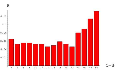
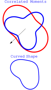
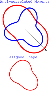
Figure 11: Distribution of the smallest angle btween a quadrupole minimum and a sextupole minimum for 324 galaxies in the north HDF.

  

Figure 12: Sketches showing the sum of quadrupole and sextupole moments when moment minima are aligned (“curved”) and when moment maxima are aligned (“aligned”).

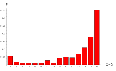
Figure 13: The distribution of quadrupole-octupole orientation in the HDF North for 324 z-selected galaxies).

In addition to the magnitude of the sextupole moment, its orientation with respect to the quadrupole moment is of particular interest to us. A plot of the relative orientation of these moments is shown in Fig. 12 for 324 z-selected galaxies from the Hubble north field. An angle of 0^o indicates that one of the sextupole minima is aligned with a quadrupole minimum. We will call such galaxies “curved”. When the angle is 30^o one of the sextupole maxima is aligned with a quadrupole maximum. We shall call such galaxies “aligned” see Fig. 12 .

The orientation of the octupole moment with respect to the quadrupole is shown for the same sample in Fig. 13. The orientation that results from an induced kick is at 0^o; the orientation that occurs naturally, and would be present for example in a bi-Gaussian distribution is oriented at 45^o. Though the octupole story is of some interest, and the small bump at 0^o in the angular distribution is tantalizing, statistics at this time are too small to draw meaningful conclusions and we will not discuss the octupole further.

  

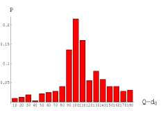
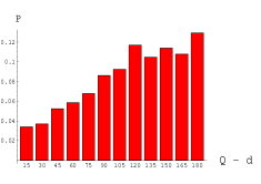
Figure 14: The distribution of the orientation angle for $d_{0}$ (left plot) and $d$ (right plot). $0^{\circ}$ is defined by the direction to the scattering center as determined by the quadrupole and sextupole moment.

Fig. 14 shows the orientation of the $d$ coefficient with respect to the quadrupole coefficient.

VI Clumping of curved and aligned galaxies

The interesting observation about “curved” galaxies is that they seem to be clumped. There are two ways to study this. The first method is to calculate the number of curved neighbors of each curved galaxy that lie within a certain distance and compare this to a distribution of the same number ($N_{c}$) of randomly chosen galaxies. We draw a circle of a fixed radius about each curved galaxy in the field. If the circle intersects the boundary of the field we drop the galaxy from consideration. Otherwise we count the number of neighboring galaxies within each circle, and make a histogram showing the number of galaxies with one, two, three, four, and so on, neighboring galaxies inside the circle. To judge whether the observed distribution is unusual, we have compared this histogram with the average histogram from 300 sets of $N_{c}$ randomly chosen galaxies. Considering that the z-distribution of galaxies might play a role in the spatial clumping, we decided to require the randomly chosen samples to have approximately the same z-distribution as the curved set of galaxies. An example of such a histogram is shown in Fig. 15 for the North HD field. We call a galaxy “curved” if the angle between quadrupole and sextupole minima is between 0^o and 8^o (see Fig. 12 and Fig. 12).

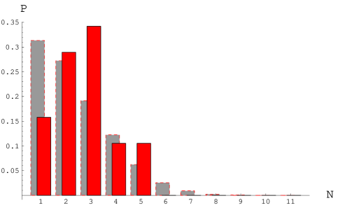
Figure 15: A “neighbors” histogram for curved galaxies for HDF North in the circle with r = 360 pixels. The background (gray) bins represent the averaged random set, the foreground histogram corresponds to a curved set.

  

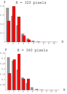
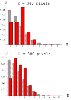
Figure 16: A “neighbors” histogram for clumped galaxies for HDF North in the circle with r = 320, 340, 360 and 380 pixels.

Fig. 16 shows four such histograms for several circle radii (in number of pixels). In this radius range (320 pixels to 380 pixels) one sees that the curved galaxy set consistently tends to have larger numbers of neighbors within its circles.

To determine the probability of finding such a systematic shift by chance we compute the total number of galaxies ( in each of these 300 randomly chosen galaxy sets ) for which the circle about a galaxy contains 3 or more neighbors. Fig. 17

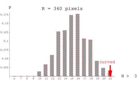
Figure 17: Histogram of numbers of galaxies in 300 randomly chosen sets having 3 or more neighbors in a circle of 360 pixels. The red arrow indicates the number of galaxies with 3 or more neighbors for the curved set.

displays the results of this study as a histogram: the label of the bins indicates numbers of circles with 3 or more neighbors. (The number corresponding to the “curved” set is indicated by an arrow.) This is done for several choices of circle radius. Typically, for the optimum radius, which is usually near 340 to 360 pixels, there will be less than 3 out of 300 sets that have as many galaxy-circles with counts equal to or greater than the original curved set. In other words, the probability of achieving the curved set by chance is equal to or smaller than 1%. Since this result holds in both fields, and the fields are independent, the probability of the observation is less than one in 10⁴.

The second method to investigate the clumping is to consider a distribution of the distances to the “nearest neighbor” for the galaxies from the “curved” set and compare it to the random sets (see Fig. 18). The horizontal axis on Fig. 18 is the distance to the ‘nearest neighbor”.

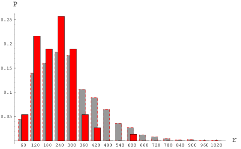
Figure 18: A distribution of the distance to the nearest neighbor for galaxies in the north HDF.

The Kholmogorov-Smirnov test gives $0.5\%$ probability that these two distributions are the same. But the situation is actually less probable than that, for two further reasons.

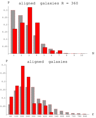
Figure 19: A “neighbors” histogram for aligned galaxies in a circle with r = 360 pixels and the average histogram for randomly chosen sets in the north HDF.

Given any distribution of background galaxy orientations, the lensing hypothesis would suggest that if the regions that are populated by dark matter clumps are giving rise to the clumping we observe, then equally well, the voids should give rise to a population of galaxies that are “straighter”, more aligned than normal. In other words, we would predict clumping of the aligned galaxies (Fig. 12 ). We have carried out the same procedure as for the “curved” galaxies for “aligned” ones and found that the “aligned” galaxies are even more clumped (Fig. 19). The probability is less than 1 %.

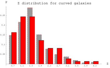
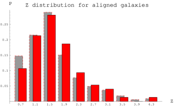
Figure 20: The red (grey) bars indicate the z-distribution of “curved” (all) galaxies, respectively .

Figure 21: The red (grey) bars indicate the z-distribution of “aligned” (all) galaxies, respectively..

That aligned galaxies are also clumped is not a trivial consequence of the fact that curved galaxies are clumped. Indeed galaxies midway between curved and aligned are not clumped. And though the aligned set is not completely independent of the curved set (it represents $\raise 2.15277pt\hbox{$\scriptstyle 1$}\kern-1.00006pt/\kern-1.49994pt\lower 1.07639pt\hbox{$\scriptstyle 4$}$ of the complement of the curved galaxies), we maintain that it is independent enough to assert that the probability of finding both clumped by chance is the product of the probability of each. With less than a 1% probability of curved galaxies being clumped and a 1% probability for aligned galaxies being clumped in both the north and south fields, the chance probability of all four events is less than 1 in a million.

  

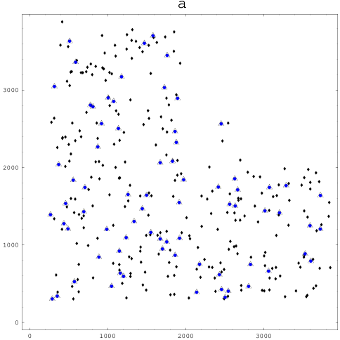
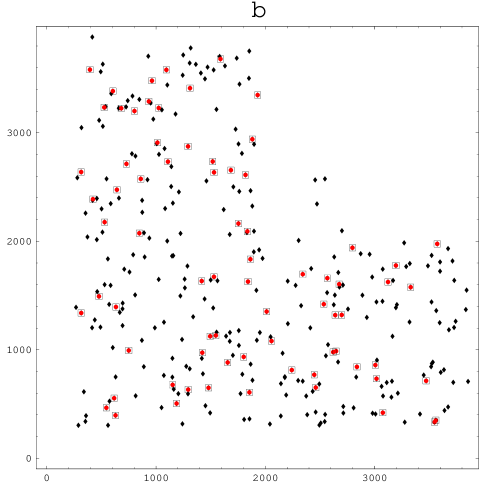
Figure 22: The HDF (North):(a) – triangles (blue dots) are curved galaxies, (b)– boxes (red dots) are “aligned” galaxies and black dots are all other background galaxies.

Fig. 21 shows and compares the z-distribution of curved galaxies with the z-distribution of all background galaxies. Fig. 21 compares the z-distribution of aligned galaxies with the z-distribution of all background galaxies. Even though the z-distributions for both curved and aligned sets are not significantly different from the average distribution we have checked the influence of z-dependence on the observed clumping. We ran the procedures described above for two cases: first, for the random sample restricted to mimic the z-distribution of a curved (aligned) set and, second, for z-“blind” random sets. The results for the probability of clumping for both cases were similar. This result was confirmed for both fields. We have also carried out an identical process, with similar results, for galaxies selected by magnitude rather than z-value. As a result of these considerations and observing the persistence of clumping under a wide variety of circumstances, we are confident that the clumping we observe is not occuring by chance. In the next section we discuss several possible alternative sources of clumping. In Fig. 22(a) we show the spatial location of the “curved” galaxies of the north field among all remaining background galaxies. In Fig. 22(b) we show the spatial distribution of “aligned” galaxies of this field with all other background galaxies.

VII Alternative explanations of clumping

Though we are comfortable in asserting that the clumping results cannot occur by chance they may be due to reasons other than lensing:

1. Instrumental

   1. The point-spread function varies over the field

   2. Pixel derived effects

2. Derived from the clumping of the background galaxies themselves

   1. Time evolution of background galaxy groups

   2. Some other group property

3. Computational

   1. The coupling of quadrupole and sextupole through $M_{21}^{T}$.

   2. Galaxy selection and analysis methods

   3. Image composition (drizzling, overlay, etc.)

We now address each of these concerns.

1(a). The point-spread function could presumably have a sextupole and quadrupole moment and these could be aligned with one another in some smoothly varying way across the image. However we feel that this is ruled out by the facts that:

Table 1: Alternative explanations for clumping of curved galaxies. Notations: + $\Rightarrow$ supports hypothesis; OK $\Rightarrow$ neutral;
NO $\Rightarrow$ contradicts hypothesis; - $\Rightarrow$ contradicts but more data required; NA $\Rightarrow$ not applicable.

Observations	Lensing	1(a) PSF	2(b) Group property	3(a) $M_{21}^{T}$	3(c) Image composition
1. Clumping of curved	+	OK	OK	NO	- Only along boundaries
2. Clumping of aligned	+	OK	OK	NO	- Only inside boundaries
3. No clumping of mid-range galaxies	+	- Could clump	OK	OK	OK
4. Mixed z content of curved clumps	+	OK	-	OK	OK
5. Curved and clumped concentrated at small a,b.	+	OK	OK	NO Prefers large $a$	OK
6. Aligned and clumped not concentrated in a,b.	+	OK	OK	OK	OK
7. Direction to scattering center varies	+	-	OK	OK	NO Pattern expected
8. Curved galaxies next to not-curved galaxies	+	NO	OK	OK	NO Pattern expected
9. Stars are round	OK	- Not enough stars	OK	OK	- Not enough stars
10. Cluster CL0024	+	NA	NA	NA	NA
11. Deduced mass magnitudes have reasonable values	+	NA	NA	NA	NA

1. the 6 stars in the Hubble north field show no sign of having a quadrupole or sextupole strength of the required magnitude;

2. mid-range galaxies (not aligned and not curved) could just as well have been clumped under this scenario and are not; and

3. the deduced directions to the scattering center are erratic.

The logic behind 2) is that if the point-spread function is causing this effect, its sextupole moment and quadrupole moment are continuously varying across the image so as to induce the observed distortion in the images. There could be isolated areas of the sky were this effect is mid-range (not necessarily aligned or curved).

1(b). We have carried out studies to see if unexpected moments are generated by dividing an image into pixels. For example, we took a known bi-Gaussian distribution and, varying the centroid, projected it onto a pixel grid. The falsely induced sextupole moment had strengths less than 10^-5. In general, there is no reason we have discerned for which pixelation effects lead to spatial correlations, since pixels (modulo pixel defects) are uniform across the field.

2(a). Since the galaxies at a slice in $z$ are known to be clumped, then if there is some age-dependent change in galaxy shapes, a shape selection criteria could be seeing an age-biased sample which could then be clumped. Since our “curved” galaxy set has the same $z$-distribution as all galaxies, the premise would appear to be false, ie galaxy curvature as we are quantifying it does not appear to evolve with time.

2(b). The premise is that galaxy groups possess some property (other than age) that effects the shape of galaxies. Perhaps there was an explosive event or set of events that extended across the group (80 kpc radius) that effected the birth process of the background galaxies. If true, it would be an unexpected and interesting result in itself. We don’t think we can rule this out yet, but with more statistics an argument to discount this scenario could be based on the fact that the curved and clumped galaxies in any given clump have a variety of z-values.

3(a). If $M_{21}^{T}$ is non-zero, a $\Delta M_{20}$ can lead to a correlated quadrupole and sextupole moment. A clumping of “curved” galaxies could result from a spatial dependence of the orientation of $M_{21}^{T}$ with respect to $\Delta M_{20}.$ A non-lensing origin of such a spatial dependence is an alternative source of clumping, but would require its own explanation, presumably one of the other alternatives among the items in our list.

3(b). Galaxy selection would appear to be blind to position in space and incapable of leading to the spatial clumping of curved or aligned galaxies

3(c). This represents our most serious concern. We suspect that we are processing this data in a way which was not anticipated by the creators of the image construction process, and we are concerned, for example, that on the boundaries of overlays, distortions could be present that would give the images a false shape. There are not enough stars in the field to rule this out using star images. Our best response to this concern is to note that the regions where curved galaxies clump do not appear to have any particular identifiable pattern, i.e. they do not appear to coincide with sub-field boundaries.

  

Figure 23: The HDF (North): triangles correspond to “curved” (left plot) and ”aligned” (right plot) galaxies and black dots on both plots are all other background galaxies.

VIII The ${\bf\large a-b}$ moment-magnitude plane

Fig. 23 (left) is what we call an $\left({\hat{a},\hat{b}}\right)$ plot for the sample of all galaxies (dots) and the set of curved galaxies (triangles). Each point on the plot corresponds to a single galaxy. The horizontal axis is the magnitude of the deduced sextupole coefficient $b$, and the vertical axis is the magnitude of the deduced quadrupole coefficient $a$. Note that galaxies having both large $a$ and large $b$ which occur in the set of all galaxies are noticeably absent in the set of curved galaxies. In the $\left({\hat{a},\hat{b}}\right)$ plot for all galaxies 40% have both $a$ and $b$-values below the mean, whereas in the $\left({\hat{a},\hat{b}}\right)$ plot for curved and clumped galaxies, 70% have both $a$ and $b$ values below that same mean.

This trend was predicted for lensing, as a consequence of considering the vector addition of the original moment and the induced moment. When the original moment is larger than the induced moment, the resulting vector tends to be aligned in the direction of the original moment, and since this angle is then divided by 2 in the case of the quadrupole moment, and by 3 in the case of the sextupole moment, the alignment with the original moment is much better than would be normally expected. On the other hand when the induced moment is larger than the original moment the argument works the same way to deduce that the alignment with the induced moment is much better than expected.

In other words, the induced curving is expected to be seen if the background moments are as small as, or smaller than the induced moment. So the population on the $a-b$ plot for curved and clumped galaxies is a strong indication of the strength of the induced moments. Of course, any other “add-on” effect will have the characteristic that it will be more noticeable for small normal or original moments, but the vector addition law with the 2$\theta$ and 3$\theta$ dependence has a remarkably sharp behavior.

“Aligned” galaxies, on the other hand, are presumed to represent galaxies that have not been altered by lensing into a mid-range or curved shape. Thus their distribution on the a-b plane should be very similar to all galaxies. This is indeed the case, as can be seen in Fig. 23 (right plot).

IX Estimate of group mass

The results of this and the following section are more speculative. We assume that the observed clumping is indeed due to lensing and attempt to deduce the properties of the lensing mass distribution. This is premature because we have not done the modeling to determine systematics and because the sample of clumped and curved galaxies is small (total of 110, both fields). On the other hand, we feel it is possible and appropriate to make order of magnitude estimates.

An estimate for the mass $M_{X}$ of the group could be written

$$M_{X}=\rho\,A_{X}=\frac{M}{d_{X}^{2}}A_{X}=\frac{M}{r_{0}^{2}}\left({\frac{r_{0}}{d_{X}}}\right)^{2}A_{X}\,,$$ (27)

where $M$ is the mass of the constituent clumps, $A_{X}$ the area of the group, and $d_{X}$ the typical separation distance of the clumps within the group. $r_{0}^{2}$ is chosen so that insertion of $M/r_{0}^{2}$ into the formula for $a$ produces a typical induced moment size for events that change the population of curved galaxies. $P_{a}\equiv\pi r_{0}^{2}/d_{X}^{2}$ can be interpreted as the probability that any particular light path receive a moment change of the required magnitude. This can be found by obtaining an estimate for the probability that the light path of any particular galaxy passing through the group receives noticeable induced moments.

To obtain this probability we have attempted to identify the clumped parts of the field (which is justified since we know it is indeed clumped) and determine the fraction of the galaxy light streams which become curved when penetrating these parts. We have done this using a friends-of-friends algorithm, requiring that i) there are at least 4 curved members in a group, and ii) that to be included in a group a curved galaxy must lie within a certain distance (about 350 pixels) of other members of the group. Fig. 24 is a combination of fig. 22(a) and fig. 22(b) with the ”curved” and aligned galaxies identified as belonging to clumps connected by straight lines.

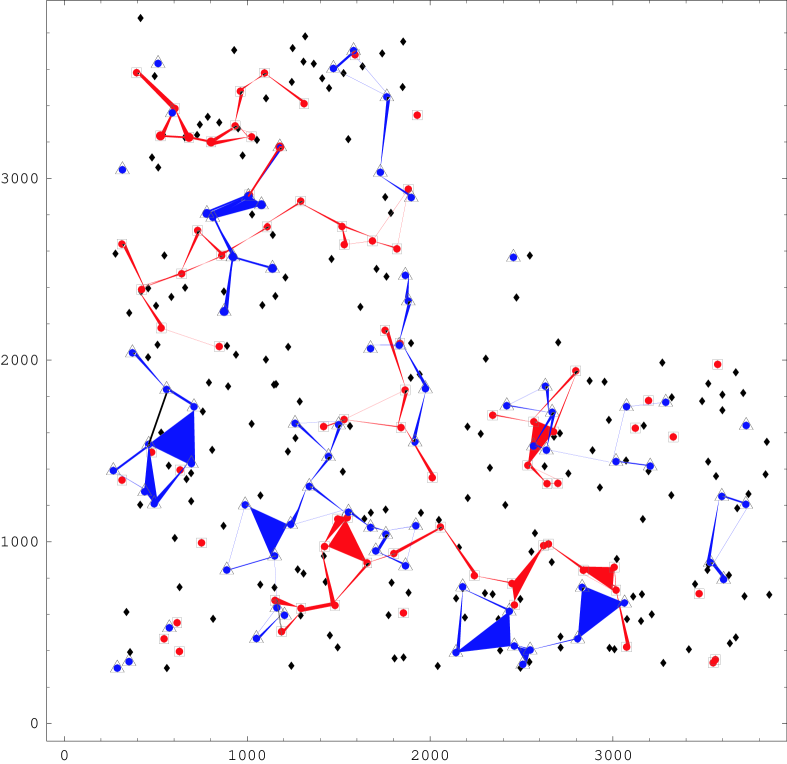
Figure 24: The HDF North red boxes are “aligned” galaxies, blue triangles are curved galaxies and black dots are all other background galaxies.

We note that we have groups with area ranging from 6 10⁵ pixels to 1.5 10⁵ pixels. Within the groups about 40% of the galaxies are curved. Outside of the groups less than 10% of the galaxies are curved. So the probability of being transformed to curved is estimated at 30%.

The transformation to curved depends on the suitability of the background galaxy (for example its moments are small enough to easily alter) times the probability that the kick is large enough. We assume that these are roughly equal, and hence get a probability of $P_{a}=0.6$ that the kick is large enough.

This yields the estimate

$$M_{X}G = \frac{a_{typ}}{4\pi}\frac{D_{TS}}{D_{TL}D_{LS}}\;P_{a}A_{X}$$

$$\approx (0.5\mbox{ to 2) }a_{typ}[{\rm pc}].$$

$a_{typ}$ has to be large enough to change moment alignments, so it must be comparable to but probably less than $\sigma_{a}$. Also we must account for the systematic weakening of moments by the point-spread function, which (see below) we would estimate at $a\approx 2\hat{a}$. For $a_{typ}\approx 0.2$, $M_{X}G\approx(0.1\mbox{ to 0.4)}\;pc\Leftrightarrow M_{X}=(2\mbox{ to 8 10}^{\mbox{12}})\;M_{\odot}$.

Moments $a$ cannot be larger than $\sigma_{a}$ because the distribution of moment strengths for curved galaxies is actually smaller than that of all galaxies. The realignment of moments can be thought of as a change of direction of the quadrupole moment or a change of direction of the sextupole moment, or a combination of both.

A distinct possibility is that there is no induced sextupole; only the quadrupole moment direction is changed leaving a sextupole behind resulting in a “curved” galaxy. One might think that higher order moments get moved along with the quadrupole because the map is linear. For example a bi-Gaussian, which has its octupole moment aligned with the ellipticity, is mapped into a bi-Gaussian which will also have its octupole moment aligned with its ellipticity. However, for sextupole moments this question is answered quantitatively by equation (13) which includes a term showing that with $b=0,$ the observed sextupole moment change will depend on the magnitude of $M_{21}^{T}$.

X Estimate of clump mass

The typical groups in the field could presumably be composed of 5 clumps of mass 10${}^{12}M_{\odot}$, 50 clumps of mass 10${}^{11}M_{\odot}$, 500 clumps of mass 10${}^{10}M_{\odot}$, 5000 clumps of mass 10${}^{11}M_{\odot}$, or some fractional combination of these. A single mass at 5 10¹² solar masses is ruled out by the erratic directions to the scattering center. We are left with this degeneracy because the expression for the induced quadrupole moment of equation (6) determines only the ratio $M/r_{0}^{2}$. Estimating the clump mass requires additional information.

Additional information can come from an analysis of the relative role played by the quadrupole and sextupole moments, according to the following considerations. It follows from equation (6) that the strength of the induced sextupole moment occurring along with the induced quadrupole moment $a_{typ}$ would be $b_{typ}=a_{typ}\;r_{G}/r_{0}$. Assuming the lensing plane is at $z=0.4$, $r_{G}\approx 0.5\;kpc$ and since $\sigma_{b}/\sigma_{a}\approx 1/5$, and as we will argue below that $a/b\approx\hat{a}/\hat{b}$, then both sextupole and quadrupole moments will be equally observable for an $r_{0}\approx 2.5\;kpc.$ Since we have estimated above that $P_{a}=\pi r_{0}^{2}/d_{X}^{2}\approx 0.6$, for this $r_{0}$ we have $d\approx 6\;kpc$ and $N=A_{X}/d_{X}^{2}\approx 500$ for the typical groups. Thus for $b_{typ}=1/5\;a_{typ}$ the estimate for the clumping mass would be $M\approx 10^{10}\;M_{\odot}$. Following this line of reasoning we have constructed the following table.

Table 2: Possible lensing parameter range.

Lensing mass /$M_{\odot}$	109	1010	1011	1012
Number of clumps in largest groups	5000	500	50	5
Typical impact parameter $r_{0}$(kpc)	0.8	2.5	8	25
$b/a$ ratio	0.6	0.2	0.06	0.02
$d_{X}$ (kpc)	2	6	20	60

From a lack of a population of localized large $b$ values, masses below 10⁹ are ruled out. Under more careful inspection and better statistics the range from a few 10⁹ through 10¹¹ should have observable consequences for $b$. The presence of lensing masses greater than 10¹¹ would be hard to numerically constrain from looking at sextupole distributions, except to know the mass is larger than the observable cut-off. However, there should be observable consequences for the quadrupole distribution, since there would be a population of larger induced moments.

In other words, we believe that a careful study of the distributions of $a$ and $b$ together with modeling should be able to provide sufficient statistical information to deduce the distribution of lensing masses.

We end this section with a discussion of systematic and random error. Important error and noise sources in any individual measurement include:

1. the systematic effects of the point-spread function and thresholding,

2. random background galaxy moments,

3. extraction of moments from the image,

4. pixelation of images, and

5. photon counting noise.

(1) The largest effect arises from thresholding and the PSF. For our galaxy cores, we estimate $M_{11}^{P}\approx M_{11}^{T}$, whence $M_{11}^{T}\approx\frac{1}{2}\hat{M}_{11}^{T}$, implying $a\approx 2\,\hat{a}$. For Gaussian shapes, $M_{22}=4M_{11}^{2}$, hence an estimate for the denominator of the expression for $\hat{b}$ is approximately $10\;\sigma^{4}\sim 2.5\;M_{22}^{T}$ and the numerator has an $\sqrt{\hat{M}_{11}^{T}}\sim\sqrt{2M_{11}^{T}}$, yielding the estimate $b\approx 2\,\hat{b}$. These are large adjustments that need careful attention, but the gross indication is that the $a/b$ ratio will suffer a smaller adjustment than either numerator or denominator and led to the use above of an estimate $a/b\approx\hat{a}/\hat{b}$.

(2) The next largest uncertainty in the $\hat{a}/\hat{b}$ ratio comes from the existence of non-zero background moments. It is a happy circumstance that there is clumping of “aligned galaxies” as well as “curved” galaxies, because the clumps of aligned galaxies are presumed to indicate a lack of lensing within their domains. Hence the distribution of galaxies behind voids will give an important base to which the galaxies behind lensing clumps can be compared. With larger statistics, one could expect to extract interesting details by studying these differences. Also it will be invaluable to have a precise knowledge of the point-spread function, including all its moments, throughout the field.

(3) We feel that our method to determine moments, validated by its ability to reveal important correlations, can be substantially improved. This is intimately related to item (1).

(4) In pixelation studies, we were surprised to find that the change of the centroid distribution was unable to produce apparent sextupole moments above the 10^-5 level. Square pixels do give rise to spurious octupole moments, and some care is required in that case.

(5) Our thresholds are typically set at approximately 175 photons per pixel. The core peaks are the order of 600 photons counts per pixel. We have not studied the effects of photon counting noise, however we would not expect its obvious random nature to affect our conclusions, and it should be substantially smaller than item (2).

XI Determination of clump radii

The probability of penetrating a clump would go like

$$\mbox{Probability}=\frac{\pi r_{L}^{2}}{d_{X}^{2}}=\frac{\pi r_{L}^{2}}{M}\frac{M}{r_{0}^{2}}\frac{r_{0}^{2}}{d_{X}^{2}}=\frac{\pi r_{L}^{2}}{M}\frac{M_{X}}{\pi r_{X}^{2}},$$ (29)

where $r_{L}$ is the lensing mass (clump mass) radius. The last ratio in this equation is fixed, so the probability depends only on the first ratio (the inverse of the projected density within a clump) which could be slowly varying. While one expects the 3-dimension density of small clumps to be larger than large clumps, the projected densities can be similar. So the probability of penetrating a clump could depend very weakly on the composition of the group.

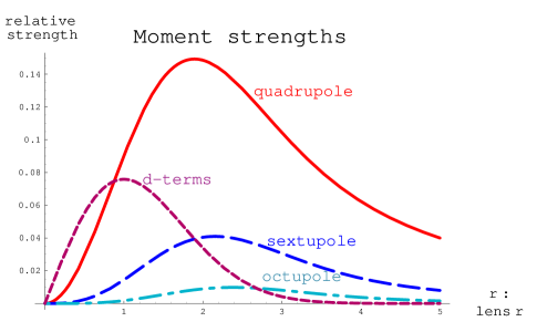
Figure 25: Strength of the quadrupole, sextupole, octupole, and cardioid-like kicks within a Gaussian clump. The horizontal axis is the radius divided by the RMS lens radius.

Penetration within a clump mass distribution will affect the strength of the induced moments and should leave a signature on the sextupole and quadrupole moment distributions. This effect is larger than one might initially expect because the sextupole moment within a clump is strongly suppressed and only reaches its asymptotic form at $r=3r_{L}.$ Fig.25 illustrates the situation fully for a Gaussian mass distribution. If $r_{L}\geq r_{G}$ ($r_{G}$ is the background galaxy light-stream footprint radius) then the interior can be well probed, and the quadrupole to sextupole ratio will remain less than

$$\frac{b}{a}\leq\frac{1}{3}\frac{r_{G}}{r_{L}}\leq\frac{1}{3}\quad.$$

If $r_{L}\leq r_{G}/3$, then as $r_{0}\to r_{G}$ the sextupole to quadrupole ratio can approach 1. In other words, for both $a$ and $b$, one must compare the difference distributions between voids and clumps. The behavior of the tail at large moments will have a different distinguishable behavior depending on the radii of the lensing masses.

The interior may also be probed with the $d$ coefficient, which is zero except within distributions. Its strength distribution is also shown in Fig. 25. Over its limited range (the maximum is at $r_{0}=r_{L})$ its value is surprisingly large. The expression for finding $d$ from moments is given by equation (II). Evidence suggesting that galaxy light paths are penetrating lensing mass distributions is present in the angular asymmetry evident in Fig. 14. The background distribution of d would be expected to be symmetric.

XII Summary

We visually examined faint images selected by the SExtractor software from the Hubble deep fields using an unusually high threshold. After filtering images with two or more maxima, we measured sextupole and quadrupole moments. The “curved” galaxies we sought were identified as those whose sextupole moment was oriented so that one of its minima was aligned within a few degrees of a quadrupole minimum. We then looked for and found an improbably large spatial clumping in each Hubble deep field of both curved and aligned galaxies. The probability of each is the order of 1%.

Our motivation and preferred hypothesis is that these galaxies were lensed by close collisions with, for example, 10¹⁰ solar mass clumps that reside within a half dozen groups of mass a few times 10¹² solar mass in each field. The projected spacing of such clumps within these groups would be about 4.5 kpc. The rms radii of the footprint in the lensing plane of the observed background galaxies is about 0.4 kpc, a factor of 10 smaller than this spacing. The cores of these galaxies could well be the order of 2 kpc, so there is a hope that the effects of light paths traveling through clump interiors may be observable through the $d$ coefficient introduced above.

We have carried out other tests that support the hypothesis that the observed clumping comes from lensing: 1) aligned galaxies were predicted and found to be clumped as strongly as curved galaxies, 2) galaxies halfway between aligned and curved were predicted and found to have no clumping, and 3) correlations were predicted to be more readily detected for galaxies with smaller moments.

We have constructed alternate hypotheses for our observations based on instrumental effects, computational effects, or other physical phenomena. The tests we have constructed and their implications for each alternative hypothesis were discussed and the results summarized in Table I. These alternatives can be eliminated (or confirmed) with more data.

Finally, the numbers that we are seeing have very interesting and plausible magnitudes, they even may be expected in the standard structure formation scenarios Davis:rj .

There are four important future studies:

1. Understand the image construction process of the deep-field images to insure that the clumping property is not an artifact of this process;

2. Simulations of small-impact parameter lensing to quantify the relationship between moment distributions and mass distributions and to discern the fraction of galaxies that are lensed but not seen;

3. Improvement of the image-analysis process, including variable thresholds and point-spread function removal;

4. Deep field studies with the additional pictures from the ACS camera on Hubble that will be available in the coming months and years.

In truth our observations should not be considered to be a subtle effect. Our samples from each Hubble deep field contains only the order of 350 background galaxies satisfying our selection criteria. About 75 of these are “curved”, and of these about 60 appear to reside in clumps. In other words, some 16% of background galaxies would be experiencing observable “small impact parameter” scattering from dark matter clumps.

These results are possible because i) the background sextupole strengths are a factor of 4 smaller than the quadrupole moments, ii) the sextupole and quadrupole moment orientations arising from lensing are correlated, and iii) one can look for clumping on the sky.

The Hubble deep fields are less than 2 min by 2 min, about $10^{-3}$ sq. deg. Projects in planning stages (eg. SNAP) have a weak lensing program of between 300 and 1000 sq. degrees with resolution comparable to the Hubble deep field observations.

If our conjecture were to be true, weak sextupole lensing could provide valuable insight into mass structure at length scales 100 times smaller than weak quadrupole lensing, at smaller scales than the Lyman alpha forest results Tegmark:2002cy .

- (1) S. Perlmutter et al., “Measurements of Omega and Lambda from 42 High-Redshift Supernovae,” Astrophys. J. 517, 565 (1999) [astro-ph/9812133], see also http://snap.lbl.gov;
- (2) A. G. Riess et al. [Supernova Search Team Collaboration], “Observational Evidence from Supernovae for an Accelerating Universe and a Cosmological Constant,” Astron. J. 116, 1009 (1998) [arXiv:astro-ph/9805201].
- (3) J. L. Tonry et al., arXiv:astro-ph/0305008.
- (4) J. L. Sievers et al., “Cosmological Parameters from Cosmic Background Imager Observations and Comparisons with BOOMERANG, DASI, and MAXIMA,” astro-ph/0205387; J. R. Bond et al., “The cosmic microwave background and inflation, then and now,” arXiv:astro-ph/0210007.
- (5) D. N. Spergel et al., “First Year Wilkinson Microwave Anisotropy Probe (WMAP) Observations: Determination of Cosmological Parameters,” arXiv:astro-ph/0302209.
- (6) M. Bartelmann and P. Schneider, Phys. Rep. 340 , 291, (2001), arXiv:astro-ph/9912508.
- (7) Y. Mellier, arXiv:astro-ph/9812172.
- (8) H. Hoekstra, H. Yee and M. Gladders, New Astron. Rev. 46, 767 (2002) [arXiv:astro-ph/0205205].
- (9) N. Kaiser, G. Wilson and G. A. Luppino, arXiv:astro-ph/0003338.
- (10) D. M. Wittman, J. A. Tyson, D. Kirkman, I. Dell’Antonio and G. Bernstein, Nature 405, 143 (2000) [arXiv:astro-ph/0003014].
- (11) Y. Mellier, L. van Waerbeke, E. Bertin, I. Tereno and F. Bernardeau, arXiv:astro-ph/0210091.
- (12) P. J. Peebles, “Principles Of Physical Cosmology,” Princeton, USA: Univ. Pr. (1994).
- (13) D. Huterer and M. S. Turner, Phys. Rev. D 64, 123527 (2001) [arXiv:astro-ph/0012510].
- (14) D. Huterer, Phys. Rev. D 65, 063001 (2002) [arXiv:astro-ph/0106399].
- (15) E. V. Linder and A. Jenkins, arXiv:astro-ph/0305286.
- (16) A. Linde, arXiv:hep-th/0211048.
- (17) R. Kallosh and A. Linde, JCAP 0302, 002 (2003) [arXiv:astro-ph/0301087].
- (18) R. Kallosh, J. Kratochvil, A. Linde, E. V. Linder and M. Shmakova, arXiv:astro-ph/0307185.
- (19) G Aldering [the SNAP Collaboration], arXiv:astro-ph/0209550.
- (20) J. Rhodes, A. Refregier and R. Massey [the SNAP Collaboration], arXiv:astro-ph/0304417; R. Massey et al., arXiv:astro-ph/0304418; A. Refregier et al., arXiv:astro-ph/0304419.
- (21) J. A. Tyson [the LSST Collaboration], Proc. SPIE Int. Soc. Opt. Eng. 4836, 10 (2002) [arXiv:astro-ph/0302102].
- (22) J. Irwin and M. Shmakova, “Cosmological Final Focus Systems”, to be published in the proceedings of 28-th Workshop on “Quantum Aspects of Beam Physics.”
- (23) R. E. Williams [the HDF Team Collaboration], arXiv:astro-ph/9607174.
- (24) S. Casertano et al., arXiv:astro-ph/0010245.
- (25) E. Bertin and S. Arnouts, Astron. Astrophys. Suppl. Ser.117, 393 (1996)
- (26) M. Davis, G. Efstathiou, C. S. Frenk and S. D. White, Astrophys. J. 292, 371 (1985).
- (27) M. Tegmark and M. Zaldarriaga, Phys. Rev. D 66, 103508 (2002) [arXiv:astro-ph/0207047].