Measuring Statistical isotropy of the CMB anisotropy

Abstract

The statistical expectation values of the temperature fluctuations of cosmic microwave background (CMB) are assumed to be preserved under rotations of the sky. This assumption of statistical isotropy (SI) of the CMB anisotropy should be observationally verified since detection of violation of SI could have profound implications for cosmology. We propose a set of measures, $\kappa_{\ell}$ ($\ell=1,2,3,\ldots$) for detecting violation of statistical isotropy in an observed CMB anisotropy sky map indicated by non zero $\kappa_{\ell}$. We define an estimator for the $\kappa_{\ell}$ spectrum and analytically compute its cosmic bias and cosmic variance. The results match those obtained by measuring $\kappa_{\ell}$ using simulated sky maps. Non-zero (bias corrected) $\kappa_{\ell}$ larger than the SI cosmic variance will imply violation of SI. The SI measure proposed in this paper is an appropriate statistics to investigate preliminary indication of SI violation in the recently released WMAP data.

The Cosmic Microwave Background (CMB) anisotropy is a very powerful observational probe of cosmology. In standard cosmology, CMB anisotropy is expected to be statistically isotropic, i.e., statistical expectation values of the temperature fluctuations $\Delta T(\hat{q})$ are preserved under rotations of the sky. In particular, the angular correlation function $C(\hat{q},\,\hat{q}^{\prime})\equiv\langle\Delta T(\hat{q})\Delta T(\hat{q}^{\prime})\rangle$ is rotationally invariant for Gaussian fields. In spherical harmonic space, where $\Delta T(\hat{q})=\sum_{lm}a_{lm}Y_{lm}(\hat{q})$ this translates to a diagonal $\langle a_{lm}a^{*}_{l^{\prime}m^{\prime}}\rangle=C_{l}\delta_{ll^{\prime}}\delta_{mm^{\prime}}$ where $C_{l}$, the widely used angular power spectrum of CMB anisotropy, is a complete description of (Gaussian) CMB anisotropy. Hence, it is important to be able to determine if the observed CMB sky is a realization of a statistically isotropic process, or not .

We propose a set of measures, $\kappa_{\ell}$ ($\ell=1,2,3,\ldots$) which for non-zero values indicate and quantify statistical isotropy violation in a CMB map. A null detection of $\kappa_{\ell}$ will be a direct confirmation of the assumed statistical isotropy of the CMB sky. It will also justify model comparison based on the angular power spectrum $C_{l}$ alone Bond,Pogosyan & Souradeep 1998, (2000). The detection of statistical isotropy (SI) violation can have exciting and far-reaching implication for cosmology. In particular, SI violation in the CMB anisotropy is the most generic signature of non-trivial geometrical and topological structure of space on ultra-large-scales. Non-trivial cosmic topology is a theoretically well motivated possibility that is being observationally probed on the largest scales only recently Ellis (1971); Lachieze-Rey & Luminet (1995); Starkman (1998); Levin (2002).

For statistically isotropic CMB sky, the correlation function

$$C(\hat{n}_{1},\hat{n}_{2})\equiv C(\hat{n}_{1}\cdot\hat{n}_{2})=\frac{1}{8\pi^{2}}\int d{\mathcal{R}}C({\mathcal{R}}\hat{n}_{1},\,{\mathcal{R}}\hat{n}_{2}),$$ (1)

where ${\mathcal{R}}\hat{n}$ denotes the direction obtained under the action of a rotation ${\mathcal{R}}$ on $\hat{n}$, and $d{\mathcal{R}}$ is a volume element of the three-dimensional rotation group. The invariance of the underlying statistics under rotation allows the estimation of $C(\hat{n}_{1}\cdot\hat{n}_{2})$ using the average of the temperature product $\widetilde{\Delta T}(\hat{n})\widetilde{\Delta T}(\hat{n}^{\prime})$ between all pairs of pixels with the angular separation $\theta$. In particular, for CMB temperature map $\widetilde{\Delta T}(\hat{q}_{i})$ defined on a discrete set of points on celestial sphere (pixels) $\hat{q}_{i}$ ($i=1,\ldots,N_{p}$)

$$\tilde{C}(\theta)\,=\,\sum_{i,j=1}^{N_{p}}\widetilde{\Delta T}(\hat{q}_{i})\widetilde{\Delta T}(\hat{q}_{j})\delta(\cos\theta-\hat{q}_{i}\cdot\hat{q}_{j})\,,$$ (2)

is an estimator of the correlation function $C(\theta)$ of an underlying SI statistics .

In the absence of statistical isotropy, $C(\hat{q},\hat{q}^{\prime})$ is estimated by a single product $\widetilde{\Delta T}(\hat{q})\widetilde{\Delta T}(\hat{q}^{\prime})$ and hence is poorly determined from a single realization. Although it is not possible to estimate each element of the full correlation function $C(\hat{q},\hat{q}^{\prime})$, some measures of statistical anisotropy of the CMB map can be estimated through suitably weighted angular averages of $\widetilde{\Delta T}(\hat{q})\widetilde{\Delta T}(\hat{q}^{\prime})$. The angular averaging procedure should be such that the measure involves averaging over sufficient number of independent ‘measurements’, but should ensure that the averaging does not erase all the signature of statistical anisotropy (as would happen in eq. (1) or eq. (2)). Another important desirable property is that the measures be independent of the overall orientation of the sky. Based on these considerations, we propose a set of measures $\kappa_{\ell}$ of statistical isotropy violation given by

$$\kappa_{\ell}=\int\!\!d\Omega\!\!\int\!\!d\Omega^{\prime}\left[\frac{(2\ell+1)}{8\pi^{2}}\!\!\int d{\mathcal{R}}\chi_{\ell}({\mathcal{R}})C({\mathcal{R}}\hat{q},{\mathcal{R}}\hat{q}^{\prime})\right]^{2}\!\!\!\!,$$ (3)

where $C({\mathcal{R}}\hat{q},\,{\mathcal{R}}\hat{q}^{\prime})$ is the two point correlation between ${\mathcal{R}}\hat{q}\,$ and ${\mathcal{R}}\hat{q}^{\prime}$ obtained by rotating $\hat{q}$ and $\hat{q}^{\prime}$ by an element ${\mathcal{R}}$ of the rotation group. The measures $\kappa_{\ell}$ involve angular average of the correlation weighed by the characteristic function of the rotation group $\chi_{\ell}({\mathcal{R}})=\sum_{M}D_{MM}^{\ell}({\mathcal{R}})$ where $D_{MM^{\prime}}^{\ell}$ are the Wigner D-functions Varshalovich et al. (1988). When ${\mathcal{R}}$ is expressed as rotation by an angle $\omega$ ( where $0\leq\omega\leq\pi$) about an axis ${\hat{r}}(\Theta,\Phi)$, the characteristic function $\chi_{\ell}({\mathcal{R}})\,\equiv\,\chi_{\ell}(\omega)=\sin{[(2\ell+1)\omega/2]}/{\sin{[\omega/2]}}$ is completely determined by $\omega$ and the volume element of the three-dimensional rotation group is given by $d{\mathcal{R}}\,=\,4\,\sin^{2}{\omega/{2}}\,d\omega\,\sin{\Theta}\,d\Theta\,d\Phi\,$. Using the identity $\int d{\mathcal{R}^{\prime}}\chi_{\ell}({\mathcal{R}^{\prime}})\chi_{\ell}({\mathcal{R}R^{\prime}})=\chi_{\ell}({\mathcal{R}})$, expression (3) can be simplified to

$$\kappa_{\ell}=\frac{(2\ell+1)}{8\pi^{2}}\int\!\!d\Omega\!\!\int\!\!d\Omega^{\prime}C(\hat{q},\hat{q}^{\prime})\!\!\int d{\mathcal{R}}\chi_{\ell}({\mathcal{R}})C({\mathcal{R}}\hat{q},{\mathcal{R}}\hat{q}^{\prime})\!\!\!\!,$$ (4)

containing only one integral over the rotation group. For a statistically isotropic model $C({\mathcal{R}}\hat{q}_{1},\,{\mathcal{R}}\hat{q}_{2})\,\equiv\,C(\hat{q}_{1},\,\hat{q}_{2})$ is invariant under rotation, and eq. (4) gives $\kappa_{\ell}\,=\,\kappa^{0}\delta_{\ell 0},$ due to the orthonormality of $\chi_{\ell}(\omega)$. Hence, $\kappa_{\ell}$ defined in eq. (3) is a measure of statistical isotropy.

The measure $\kappa_{\ell}$ has clear interpretation in harmonic space. The two point correlation $C(\hat{q},\,\hat{q}^{\prime})$ can be expanded in terms of the orthonormal set of bipolar spherical harmonics as

$$C(\hat{q},\,\hat{q}^{\prime})\,=\,\sum_{ll^{\prime}\ell M}A_{ll^{\prime}}^{\ell M}\{Y_{l}(\hat{q})\otimes Y_{l^{\prime}}(\hat{q}^{\prime})\}_{\ell M}\,,$$ (5)

where $A_{ll^{\prime}}^{\ell M}$ are the coefficients of the expansion. These coefficients are related to ‘angular momentum’ sum over the covariances $\langle a_{lm}a^{*}_{l^{\prime}m^{\prime}}\rangle$ as

$$A_{ll^{\prime}}^{\ell M}=\sum_{mm^{\prime}}\langle a_{lm}a^{*}_{l^{\prime}m^{\prime}}\rangle\,\,(-1)^{m^{\prime}}\mathfrak{C}^{\ell M}_{lml^{\prime}-m^{\prime}}\,,$$ (6)

where $\mathfrak{C}^{\ell M}_{lml^{\prime}m^{\prime}}$ are Clebsch-Gordan coefficients. The bipolar functions transform just like ordinary spherical harmonic function $Y_{\ell M}$ under rotation Varshalovich et al. (1988). Substituting the expansion eq. (5) into eq. (3) we can show that

$$\kappa_{\ell}=\sum_{ll^{\prime}M}|A_{ll^{\prime}}^{\ell M}|^{2}\geq 0\,,$$ (7)

is positive semidefinite and can be expressed in the form

$$\kappa_{\ell}=\frac{2\ell+1}{8\pi^{2}}\!\!\int\!\!d{\mathcal{R}}\chi_{\ell}({\mathcal{R}})\sum_{lml^{\prime}m^{\prime}}\langle a_{lm}a^{*}_{l^{\prime}m^{\prime}}\rangle\langle a_{lm}a^{*}_{l^{\prime}m^{\prime}}\rangle^{\mathcal{R}}\!\!,$$ (8)

where $\langle\ldots\rangle^{\mathcal{R}}$ is computed in a frame rotated by ${\mathcal{R}}$. When SI holds $\langle a_{lm}a^{*}_{l^{\prime}m^{\prime}}\rangle=C_{l}\delta_{ll^{\prime}}\delta_{mm^{\prime}}$, implying $A_{ll^{\prime}}^{\ell M}=(-1)^{l}C_{l}(2l+1)^{1/2}\,\delta_{ll^{\prime}}\,\delta_{\ell 0}\,\delta_{M0}$. The coefficients $A_{ll}^{00}$ represent the statistically isotropic part of a general correlation function. They also represent the statistically isotropic part of any arbitrary correlation function. The coefficients $A_{l_{1}l_{2}}^{\ell M}$ are inverse-transform of the two point correlation

$$A_{l_{1}l_{2}}^{\ell M}\,=\,\int d\Omega\int d\Omega^{\prime}\,C(\hat{n},\,\hat{n}^{\prime})\,\{Y_{l_{1}}(\hat{n})\otimes Y_{l_{2}}(\hat{n}^{\prime})\}_{\ell M}^{*}.$$ (9)

The symmetry $C(\hat{n},\hat{n}^{\prime})=C(\hat{n}^{\prime},\hat{n})$ implies

$$A_{l_{2}l_{1}}^{\ell M}\,=\,(-1)^{(l_{1}+l_{2}-\ell)}A_{l_{1}l_{2}}^{\ell M},\quad A_{ll}^{\ell M}\,=\,A_{ll}^{\ell M}\,\,\delta_{\ell,2k},\quad k=0,\,1,\,2,\,\cdots.$$ (10)

Recently, the Wilkinson Microwave Anisotropy Probe (WMAP) has provided high resolution (almost) full sky maps of CMB anisotropy Bennet et al. (2003) from which $\kappa_{\ell}$ can be measured. Given a single independent CMB map, $\widetilde{\Delta T}(\hat{q})$ we need to look for violation of statistical isotropy. Formally, the estimation procedure involves averaging the product of temperature at pairs of pixels obtained by rotating a given pair of pixels by an angle $\omega$ around a sufficiently large sample of rotation axes. The integral in the braces in eq. (3) is estimated by summing up the terms for different values of $\omega$ weighed by the characteristic function. We can define an estimator for $\kappa_{\ell}$ as

$$\tilde{\kappa}_{\ell} =\tilde{\kappa}_{\ell}^{B}-{\mathfrak{B}}_{\ell},$$

$$\tilde{\kappa}_{\ell}^{B} =\frac{(2\ell+1)}{8\pi^{2}}\sum_{i,j=1}^{N_{p}}\widetilde{\Delta T}(\hat{q}_{i})\,\widetilde{\Delta T}(\hat{q}_{j})\sum_{m=1}^{N_{w}}\chi_{\ell}(w_{m})\sum_{n=1}^{N_{r}}\widetilde{\Delta T}({\mathcal{R}}_{mn}\hat{q}_{i})\widetilde{\Delta T}({\mathcal{R}}_{mn}\hat{q}_{j})\,,$$ (11)

where as described below ${\mathfrak{B}}_{\ell}\equiv\langle\tilde{\kappa}_{\ell}^{B}\rangle$ accounts for the ‘cosmic bias’ for the biased estimator $\tilde{\kappa}_{\ell}^{B}$. As with the sky, the rotation group is also discretized as ${\mathcal{R}}_{mn}$ where $m=1,\ldots,N_{w}$ is an index of equally spaced intervals in rotation angle $w$ and $n=1,\ldots,N_{r}$ indexes a set of equally spaced directions in the sky. While we have also implemented this real space computation, practically, we find it faster to estimate $\kappa_{\ell}$ in the harmonic space by taking advantage of fast methods of spherical harmonic transform of the map. In harmonic space, we first define an unbiased estimator for the bipolar harmonic coefficients based on eq. (6) and then estimate $\kappa_{\ell}$ using eq. (7)

$$\tilde{A}_{ll^{\prime}}^{\ell M}=\sum_{mm^{\prime}}a_{lm}a_{l^{\prime}m^{\prime}}\,\,\mathfrak{C}^{\ell M}_{lml^{\prime}m^{\prime}}\,\quad\tilde{\kappa}_{\ell}=\sum_{ll^{\prime}M}\left|\tilde{A}_{ll^{\prime}}^{\ell M}\right|^{2}-{\mathfrak{B}}_{\ell}\,.$$ (12)

Assuming Gaussian statistics of the temperature fluctuations, the cosmic bias is given by Hajian & Souradeep (2003)

$$\langle\tilde{\kappa}_{\ell}^{B}\rangle-\kappa_{\ell}=\sum_{l_{1},l_{2}}\sum_{m_{1},m_{1}^{\prime}}\sum_{m_{2},m_{2}^{\prime}} \,\left[\langle a^{*}_{l_{1}m_{1}}a_{l_{1}m_{1}^{\prime}}\rangle\langle a^{*}_{l_{2}m_{2}}a_{l_{2}m_{2}^{\prime}}\rangle+\langle a^{*}_{l_{1}m_{1}}a_{l_{2}m_{2}^{\prime}}\rangle\langle a^{*}_{l_{2}m_{2}}a_{l_{1}m_{1}^{\prime}}\rangle\right]$$ (13)

$${}\times\sum_{M}\mathfrak{C}^{\ell M}_{l_{1}m_{1}l_{2}m_{2}}\mathfrak{C}^{\ell M}_{l_{1}m_{1}^{\prime}l_{2}m_{2}^{\prime}}\,.$$

Given a single CMB sky-map, the individual elements of the $\langle a_{lm}a^{*}_{l^{\prime}m^{\prime}}\rangle$ covariance are poorly determined. So we can correct for the bias ${\mathfrak{B}}_{\ell}$ that arises from the SI part of correlation function where

$${\mathfrak{B}}_{\ell}\equiv\langle\tilde{\kappa}_{\ell}^{B}\rangle_{{}_{\rm SI}}=(2\ell+1)\,\sum_{l_{1}}\sum_{l_{2}=|\ell-l_{1}|}^{\ell+l_{1}}C_{l_{1}}C_{l_{2}}\left[1+(-1)^{\ell}\,\delta_{l_{1}l_{2}}\right]\,.$$ (14)

Hence, for SI correlation, the estimator $\tilde{\kappa}_{\ell}$ is unbiased, i.e., $\langle\tilde{\kappa}_{\ell}\rangle=0$.

Assuming Gaussian CMB anisotropy, the cosmic variance of the estimators $\tilde{A}_{ll^{\prime}}^{\ell M}$ and $\tilde{\kappa}_{\ell}$ can be obtained analytically for full sky maps. The cosmic variance of the bipolar coefficients

$$\sigma^{2}(\tilde{A}_{l_{1}l_{2}}^{\ell M})=\sum_{m_{1},m_{1}^{\prime}}\sum_{m_{2},m_{2}^{\prime}}\, \left[\langle a_{l_{1}m_{1}}a_{l_{1}m_{1}^{\prime}}\rangle\langle a_{l_{2}m_{2}}a_{l_{2}m_{2}^{\prime}}\rangle+\langle a_{l_{1}m_{1}}a_{l_{2}m_{2}^{\prime}}\rangle\langle a_{l_{2}m_{2}}a_{l_{1}m_{1}^{\prime}}\rangle\right]$$ (15)

$${}\times\mathfrak{C}^{\ell M}_{l_{1}m_{1}l_{2}m_{2}}\mathfrak{C}^{\ell M}_{l_{1}m_{1}^{\prime}l_{2}m_{2}^{\prime}},$$

which, for SI correlation, further simplifies to

$$\sigma^{2}_{{}_{\rm SI}}(\tilde{A}_{l_{1}l_{2}}^{\ell M})=C_{l_{1}}\,C_{l_{2}}\,\left[1+(-1)^{\ell}\,\delta_{l_{1}l_{2}}\right]\,\sum_{m_{1},m_{2}}(-1)^{m_{1}+m_{2}}\mathfrak{C}^{\ell M}_{l_{1}m_{1}l_{2}m_{2}}\mathfrak{C}^{\ell M}_{l_{1}m_{1}^{\prime}l_{2}m_{2}^{\prime}}.$$ (16)

Note that for $l_{1}=l_{2}$ the cosmic variance is zero for odd $\ell$ due to eq. (10) arising from symmetry of $C(\hat{q},\hat{q}^{\prime})$.

A similar but more tedious computation of $105$ terms of the $8$-point correlation function yields an analytic expression for the cosmic variance of $\tilde{\kappa}_{\ell}$ Hajian & Souradeep (2003). For SI correlation, the cosmic variance for $\ell>0$ is given by

$$\sigma^{2}_{{}_{\rm SI}}(\tilde{\kappa}_{\ell})=\sum_{l:2l\geq\ell}\!\!4\,C_{l}^{4}\left[2\frac{(2\ell+1)^{2}}{2l+1}+(-1)^{\ell}(2\ell+1)+(1+2(-1)^{\ell})F_{ll}^{\ell}\right]$$ (17)

$${}+\sum_{l_{1}}\sum_{l_{2}=|\ell-l_{1}|}^{\ell+l_{1}}\!\!\!4\,C_{l_{1}}^{2}\,C_{l_{2}}^{2}\left[(2\ell+1)+F_{l_{1}l_{2}}^{\ell}\right]+\,8\sum_{l_{1}}\,\frac{(2\ell+1)^{2}}{2l_{1}+1}\,C_{l_{1}}^{2}\left[\sum_{l_{2}=|\ell-l_{1}|}^{\ell+l_{1}}C_{l_{2}}\right]^{2}$$

$${}+16\,(-1)^{\ell}\,\sum_{l_{1}:2l_{1}\geq\ell}\,\frac{(2\ell+1)^{2}}{2l_{1}+1}\,\sum_{l_{2}=|\ell-l_{1}|}^{\ell+l_{1}}C_{l_{1}}^{3}C_{l_{2}},$$

$${\rm where} F_{l_{1}l_{3}}^{\ell}=\!\!\!\!\sum_{m_{1}m_{2}=-l_{1}}^{l_{1}}\,\sum_{m_{3}m_{4}=-l_{3}}^{l_{3}}\sum_{M,M^{\prime}=-\ell}^{\ell}C^{\ell M}_{l_{1}-m_{1}l_{3}-m_{3}}C^{\ell M}_{l_{1}m_{2}l_{3}m_{4}}C^{\ell M^{\prime}}_{l_{3}m_{4}l_{1}m_{1}}C^{\ell M^{\prime}}_{l_{3}-m_{3}l_{1}-m_{2}}.$$ (18)

Numerically, it is advantageous to rewrite $F_{ll^{\prime}}^{\ell}$ in a series involving $9$-j symbols. The expressions for variance and bias are valid for full sky CMB maps. For observed maps one has to contend to incomplete or non uniform sky coverage. In such cases one would estimate the cosmic bias and variance from averaging over many independent realizations simulated CMB sky from the same underlying correlation function. Fig. 1 shows the measurement of $\kappa_{\ell}$ in a SI model with flat band power spectrum. The bias and variance is estimated from making measurements on $50$ independent random full-sky maps using the HEALPix . The cosmic bias and variance obtained from these realizations match the analytical results. Just as in the case of cosmic bias, the cosmic variance of $\kappa_{\ell}$ at odd multipoles is smaller. The figure clearly shows that the envelope of cosmic variance for odd and even mulitpole converge at large $\ell$. For a constant $l(l+1)C_{l}$ angular power spectrum the $\sigma_{{}_{\rm SI}}(\tilde{\kappa}_{\ell})$ falls off approximately as $1/\ell$ at large $\ell$. (The absence of dipole and monopole in the maps affects $\kappa_{\ell}$ for $\ell<4$ leading to the apparent rise in cosmic variance at $\ell<4$ seen in Fig 1.)

The bias and cosmic variance depends on the total SI angular power spectrum of the signal and noise $C_{l}=C_{l}^{S}+C_{l}^{N}$. Hence, where possible, prior knowledge of the expected $\kappa_{\ell}$ signal should be used to construct multipole space windows to weigh down the contribution from the region of multipole space where SI violation is not expected, e.g., the generic breakdown of statistical isotropy due to cosmic topology. The underlying correlation patterns in the CMB anisotropy in a multiply connected universe is related to the the symmetry of Dirichlet domain  Wolf (1994); Vinberg (1993). In a companion paper, we study the $\kappa_{\ell}$ signal expected in flat, toroidal models of the universe and connect the spectrum to the principle directions in the Dirichlet domain Hajian & Souradeep (2003). SI violation arising from cosmic topology is usually limited to low multipoles. A wise detection strategy would be to smooth CMB maps to the low angular resolution. When searching for specific form of SI violation, linear combinations of $\kappa_{\ell}$ can be used to optimize signal to noise. Before ascribing the detected breakdown of statistical anisotropy to cosmological or astrophysical effects, one must carefully account for and model into the SI simulations other mundane sources of SI violation in real data, such as, incomplete and non-uniform sky coverage, beam anisotropy, foreground residuals and statistically anisotropic noise.

In summary, the $\kappa_{\ell}$ statistics quantifies breakdown of SI into a set of numbers that can be measured from the single CMB sky available. The $\kappa_{\ell}$ spectrum can be measured very fast even for high resolution CMB maps. The statistics has very clear interpretation as quadratic combinations of off-diagonal correlations between $a_{lm}$ coefficients. Signal SI violation is related to underlying correlation patterns. The angular scale on which the off-diagonal correlations (patterns) occur is reflected in the $\kappa_{\ell}$ spectrum. As a tool for detecting cosmic topology (more generally, cosmic structures on ultra-large scales), the $\kappa_{\ell}$ spectrum has the advantage of being independent of overall orientation of the correlation pattern. This is particularly suited for search for cosmic topology since the signal is independent of the orientation of the DD. (However, orientation information is available in the $A^{\ell M}_{l_{1}l_{2}}$.) The recent all sky CMB map from WMAP is an ideal data set where one can measure statistical isotropy. Interestingly, there are hints of SI violation in the low multipole of WMAP Tegmark et al. (2003); de Oliveira-Costa et al. (2003); Eriksen et al. (2003). Hence is of great interest to make a careful estimation of SI violation in the WMAP data via $\kappa_{\ell}$ spectrum. This work is in progress and results will be reported elsewhere Hajian et al. (2003). This approach complement direct search for signature of cosmic topology Cornish,Spergel & Starkman (1998).

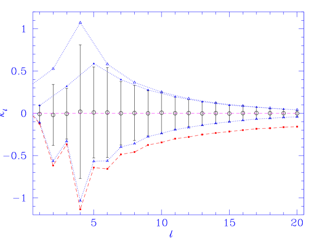
Figure 1: The figure shows the bias corrected ‘measurement’ of $\kappa_{\ell}$ of a SI CMB sky with a flat band power spectrum smoothed by a Gaussian beam ($l(l+1)C_{l}=\exp(-l^{2}/18^{2})$. The cosmic error, $\sigma({\kappa_{\ell}})$, obtained using $50$ independent realizations of CMB (full) sky map match the analytic results shown by lower dotted curve with stars. The upper dotted curves separately outline the cosmic error envelope for odd multipoles (filled triangles) and for even multipoles (empty triangles) to explicitly highlight their convergence. Violation of SI will be indicated by non-zero $\kappa_{\ell}$ measured in an observed CMB map in excess of $\sigma({\kappa_{\ell}})$ given by the $C_{l}$ of the map. The lower dashed curve (filled squares) shows the cosmic error for ideal unit flat band power spectrum ($l(l+1)C_{l}=1$) with no beam smoothing. The curve falls off roughly at $1/\ell$ at large $\ell$.

References

• Bennet et al. (2003) C. L. Bennet et al., 2003, Astrophys. J (in press) (astro-ph/0302207)
• Bond,Pogosyan & Souradeep 1998, (2000) Bond,J. R., Pogosyan, D. & Souradeep,T. 1998, Class. Quant. Grav. 15, 2671 ; ibid. 2000, Phys. Rev. D 62,043005;2000, Phys. Rev. D 62,043006
• Bunn & Scott (2000) Bunn, E. and Scott, D. 2000 M.N.R.A.S., 313, 331
• Cornish,Spergel & Starkman (1998) Cornish, N.J., Spergel, D.N. & Starkman, G. D. 1998, Class. Quantum Grav., 15, 2657
• Ellis (1971) Ellis,G. F. R. 1971, Gen. Rel. Grav. 2, 7
• Eriksen et al. (2003) Eriksen, H. K., Hansen, F. K., Banday A. J., Gorski, K. M., Lilje, P. B. 2003, preprint (astro-ph/0307507)
• Ferreira & Magueijo (1997) Ferreira, P. G. & Magueijo, J. 1997, Phys. Rev. D56, 4578
• G rski, Hivon & Wandelt (1999) GΓ³rski,K. M., Hivon, E., Wandelt, B. D. 1999, in ”Evolution of Large-Scale Structure”, eds. A.J. Banday, R.S. Sheth and L. Da Costa, PrintPartners Ipskamp, NL, pp. 37-42 (also astro-ph/9812350)
• Hajian & Souradeep (2003) Hajian, A. & Souradeep, T., preprint (astro-ph/0301590)
• Hajian & Souradeep (2003) Hajian, A. & Souradeep, T., in preparation
• Hajian et al. (2003) Hajian,Β A. Souradeep,Β T., Cornish,Β N., Starkman,Β G. and Spergel,Β D.Β N. 2003, in preparation.
• Lachieze-Rey & Luminet (1995) Lachieze-Rey, M. and Luminet,J. -P. 1995, Phys. Rep. 25, 136
• Levin (2002) Levin, J. 2002, Phys. Rep. 365, 251
• Souradeep (2000) Souradeep,T. 2000, in β€˜The Universe’, eds. Dadhich, N. & Kembhavi, A., Kluwer
• Starkman (1998) Starkman, G. Class. 1998, Quantum Grav. 15, 2529
• Tegmark et al. (2003) Tegmark, M., de Oliveira-Costa, A. & Hamilton, A. 2003, preprint, (astro-ph/0302496)
• de Oliveira-Costa et al. (2003) de Oliveira-Costa,Β A., Tegmark,Β M., Zaldarriaga,Β M. & Hamilton,Β A. 2003, preprint, (astro-ph/0307282)
• Varshalovich et al. (1988) Varshalovich, D. A., Moskalev, A. N., Khersonskii, V. K., 1988 Quantum Theory of Angular Momentum (World Scientific)
• Vinberg (1993) Vinberg,E. B. 1993, Geometry II – Spaces of constant curvature, (Springer-Verlag)
• Wolf (1994) Wolf, J. A. 1994, Space of Constant Curvature (5th ed.), (Publish or Perish, Inc.)
Refer to caption