Myths and Truths Concerning Estimation of Power Spectra: The Case for a Hybrid Estimator

Abstract

It is widely believed that maximum likelihood estimators must be used to provide optimal estimates of power spectra. Since such estimators require the inversion and multiplication of $N_{d}\times N_{d}$ matrices, where $N_{d}$ is the size of the data vector, maximum likelihood estimators require at least of order $N_{d}^{3}$ operations and become computationally prohibitive for $N_{d}$ greater than a few tens of thousands. Because of this, a large and inhomogeneous literature exists on approximate methods of power spectrum estimation. These range from manifestly sub-optimal, but computationally fast methods, to near optimal but computationally expensive methods. Furthermore, much of this literature concentrates on the power spectrum estimates rather than the equally important problem of deriving an accurate covariance matrix. In this paper, I consider the problem of estimating the power spectrum of cosmic microwave background (CMB) anisotropies from large data sets. Various analytic results on power spectrum estimators are derived, or collated from the literature, and tested against numerical simulations. An unbiased hybrid estimator is proposed that combines a maximum likelihood estimator at low multipoles and pseudo-$C_{\ell}$ estimates at high multipoles. The hybrid estimator is computationally fast (i.e. it can be run on a laptop computer for Planck sized data sets), nearly optimal over the full range of multipoles, and returns an accurate and nearly diagonal covariance matrix for realistic experimental configurations (provided certain conditions on the noise properties of the experiment are satisfied). It is argued that, in practice, computationally expensive methods that approximate the ${\cal O}(N_{d}^{3})$ maximum likelihood solution are unlikely to improve on the hybrid estimator, and may actually perform worse. The results presented here can be generalised to CMB polarization and to power spectrum estimation using other types of data, such as galaxy clustering and weak gravitational lensing.

Key words: Methods: data analysis, statistical; Cosmology: cosmic microwave background, large-scale structure of Universe

1 Introduction

The estimation of power spectra from various types of data is becoming increasingly important in cosmology. There are three main reasons for this. Firstly, there has been an explosion in the size and quality of cosmological data sets, for example, the detailed maps of the CMB sky from WMAP (Bennett et al. 2003), the 2dFGRS (Colless et al. 2001) and SDSS galaxy redshift survey (Zehavi et al. 2002; Tegmark et al. 2004). With such large data sets it is now possible to measure power spectra accurately over a wide range of angular and spatial scales. Secondly, the power spectrum is a simple two-point statistic and so it is natural that more effort has been devoted to optimal methods of power spectrum estimation rather than to optimal estimators for higher order statistics. Thirdly, in most realisations of the inflationary scenario, the fluctuations generated during the inflationary phase are predicted to be Gaussian (see e.g. Liddle and Lyth, 2000, for a review). If the fluctuations are Gaussian, and as long as they remain linear, all of the information pertaining to the fluctuations is contained in the power spectrum. In this case, estimation of the power spectrum can be viewed as a form of lossless data compression, reducing, for example, $10^{7}$ measurements of the CMB temperature differences $\Delta T_{i}$ into $2000$ or so values of the angular power spectrum $C_{\ell}$ (see e.g. Tegmark 1997). This form of data compression is invaluable, since physical parameters of interest (matter densities, spectral indices etc) can be estimated from the power spectrum and its covariance matrix, rather than from the pixel values themselves.

One of the earliest applications of power spectrum analysis to cosmology was Yu and Peebles’ (1969) analysis of the angular distribution of rich clusters of galaxies. These authors applied what is now (unfortunately) commonly referred to as a ‘pseudo-$C_{\ell}$’ estimator (see Section 2). In the rest of this paper, we will discuss the specific problem of power spectrum estimation of CMB temperature anisotropies, although many of the results and remarks are applicable to other types of data, such as galaxy clustering. A comprehensive analysis of pseudo-$C_{\ell}$ estimators was given by Peebles (1973) and an application to the angular clustering of galaxies can be found in Peebles and Hauser (1974). Although it was well known that pseudo-$C_{\ell}$ estimators are sub-optimal, little work was done to develop more optimal power spectrum estimators until recently (the paper by Feldman, Kaiser and Peacock, 1994, on power spectrum analysis of redshift surveys is a noteable exception). Hamilton (1997a, b), Tegmark (1997) and Bond, Jaffe and Knox (1998) constructed estimators that are optimal, in the sense that they find the power spectrum that maximises the likelihood function given the data. However, there is a fundamental problem with these maximum likelihood estimators. Given a data vector of length $N_{d}$, optimal estimators require the inversion of $N_{d}\times N_{d}$ matrices. Since a matrix inversion requires ${\cal O}(N_{d}^{3})$ operations, brute force application of maximum likelihood estimators becomes impractical for $N_{d}$ greater than a few tens of thousands (see e.g. Borrill 1999a,b). As a result, a large number of papers have appeared in the last few years that discuss various solutions to the problem of power spectrum estimation from large data sets.

These papers can be grouped, roughly, into the following categories:

(i) Pseudo-$C_{\ell}$ estimators: These are straightforward variants of the methods described by Peebles (1973). A discussion of a pseudo-$C_{\ell}$ estimator (hereafter PCL) applied to CMB experiments is given by Wandelt, Hivon and Górski (2001) and Hivon et al. (2002). Variants designed to recover the true shape of the power spectrum from apodised regions of the sky are discussed by Hansen, Górski and Hivon (2002) and Hansen and Górski (2003). These estimators can be evaluated using fast spherical transforms (e.g. Muciaccia, Natoli and Vittorio 1997) for which the number of operations scale as $N_{d}^{3/2}$. Even for data vectors of the length expected from the Planck mission (Bersannelli et al. 1996), $N_{d}\sim 10^{7}$, it is possible to evaluate a PCL estimator using a laptop computer (see e.g. Balbi et al. 2002). A PCL estimator was used in the analysis of the WMAP data (Hinshaw et al. 2003)

A related class of sub-optimal estimators use fast evaluation of the two-point correlation function, which can then be transformed to give an estimate of the power spectrum. Methods of this type, designed for the analysis of CMB anisotropies are described by Szapudi et al. (2001a) and by Szapudi, Prunet and Colombi (2001b). A generalisation of these methods to the analysis of CMB polarization is discussed by Chon et al. (2003). We group this type of estimator along with the PCL methods described in the previous paragraph because they are almost mathematically equivalent.

(ii) Maximum likelihood estimators: Given a data vector $x_{i}$ of length $N_{d}$, and assuming that the $x_{i}$ are Gaussian distributed, we can define a likelihood function

$${\cal L}(C_{\ell}|{\bf x})={{\rm exp}\left(-{1\over 2}x^{T}C^{-1}x\right)\over(2\pi)^{N_{d}/2}|C|^{1/2}},$$ (1)

where $C_{\ell}$ is the power spectrum to be estimated. The covariance matrix $C$ in (1) is

$$C_{ij}=\langle x_{i}x_{j}\rangle=S_{ij}(C_{\ell})+N_{ij},$$ (2)

where $S$ is the signal covariance matrix and $N$ is the noise matrix. A maximum likelihood estimator finds the $C_{\ell}$, or an approximation to the $C_{\ell}$, that maximises the likelihood (1).

Two types of maximum likelihood (herafter ML) estimator have been discussed widely. In the first, which we will refer to as NRML, the power spectrum that maximises the likelihood function is found iteratively using a Newton-Raphson algorithm (Bond, Jaffe and Knox 1998; Ruhl et al. 2003). In the second, which we will refer to as QML, a quadratic estimator is defined based on an assumed form for $C_{\ell}$ which is equivalent to a maximum likelihood solution if the guess for $C_{\ell}$ is close to the true power spectrum (e.g. Tegmark 1997). From equation (1) one can see that both the NRML and QML estimators require the inverse and determinant of the covariance matrix $C$ and so require of ${\cal O}(N_{d}^{3})$ operations.

Various methods have been proposed to speed up the computation of ML estimators. Oh, Spergel and Hinshaw (1999) use a conjugate gradient algorithm with a carefully chosen preconditioner to avoid direct invertion of the matrix (2). Doré, Knox and Peel (2001) propose an NRML estimator based on hierarchical decomposition of a large map into sub-maps of various resolutions, though this method has the disadvantage of a loss of resolution in the power spectrum estimates. An iterative multi-grid method is described by Pen (2003) and a method that uses Monte Carlo Markov Chains is described by Jewell, Levin and Anderson (2002).

(iii) Harmonic and Ring-torus Estimators: For a Planck-type scanning strategy, a ML solution for the spherical harmonic coefficients $a_{\ell m}$ can be determined from the Fourier transform of the temperature differences on a set of rings on the sky (van Leeuwen et al. 2002; Challinor et al. 2002). The data vector $x_{i}$ in equation (1) is then the set of harmonic coefficients $a_{\ell m}$. This type of ‘harmonic’ method avoids the need to construct pixelised maps of the temperature differences on the sky and can account for asymmetric beams and certain types of correlated noise. However, a brute force application of the harmonic method would require of ${\cal O}(\ell_{\rm max}^{6})$ operations, where $\ell_{\rm max}$ is the highest multipole under consideration, and so is not computationally feasible for high multipoles. The operation count can be reduced for simple scanning strategies and by using conjugate gradient techniques, but so far little work has been done along these lines. A related method is described by Wandelt and Hansen (2003), who show that for special scanning geometries the time-ordered data (TOD) can be wrapped onto a ring torus. In this case, the ML solution for $C_{\ell}$ can be found in ${\cal O}(N^{2}_{d})$ operations using the fast spherical convolution algorithm described by Wandelt and Górski (2001). Even if the scanning geometry of an experiment does not satisfy the precise conditions for an ${\cal O}(N^{2}_{d})$ solution, Wandelt and Hansen argue that the ring-torus method can be useful in determining a preconditioner to speed up the computation of the exact ML solution.

Given the large number of methods described in the previous paragraphs, what is the best way to estimate a power spectrum from a large data set, including realistic sources of errors? In the view of this author, the work summarised above suggests two approaches:

${\bf(A)}$ Application of a computationally expensive ML method that can account for various sources of error, such as correlated receiver noise, beam asymmetries etc. For a large ($N_{d}\lower 2.15277pt\hbox{$\;\buildrel>\over{\sim}\;$}10^{6}$) data set, the noise matrix $N$ in equation (2) is neither calculable nor storeable, and so if correlated noise is to be taken into account the method would have to be based on (and exploit symmetries in) the TOD.

${\bf(B)}$ Application of a fast PCL-based method which can be used to derive an analytic covariance matrix under certain simplifying assumptions (e.g. diagonal noise matrix, symmetric beams). Real-world complications can then be treated as perturbations to the covariance matrix, which can be estimated by running a large number of Monte Carlo simulations.

The point of view adopted in this paper is that approach (B) is preferable to approach (A) and that there has been an over-emphasis in the literature on computationally expensive maximum likelihood methods. There are several reasons for taking this viewpoint:

(a) Does a maximum likelihood estimator lead to a significant reduction in the error bars compared to using a PCL estimator? In some limits it is possible to prove that a PCL is statistically equivalent to a ML estimator (Sections 3 and 5). Furthermore, for realistic experiments there may be ‘irreducible’ errors on the power spectrum estimates that dominate over any minor differences between estimators. For example, in the WMAP experiment beam calibration uncertainties are the dominant source of error in the range $100\lower 2.15277pt\hbox{$\;\buildrel<\over{\sim}\;$}\ell\lower 2.15277pt\hbox{$\;\buildrel<\over{\sim}\;$}600$ and residual Galactic emission is the dominant source of error at multipoles $\ell\lower 2.15277pt\hbox{$\;\buildrel<\over{\sim}\;$}10$ (Hinshaw et al. 2003).

(b) As discussed above, for many purposes, a power spectrum is simply a convenient form of data compression to enable fast estimation of a small number of physical parameters. But to determine the physical parameters we must be able to write down a likelihood function, which requires at least an accurate covariance matrix for the power spectrum estimates and preferably an accurate model for the shape of the likelihood function (see e.g. Bond, Jaffe and Knox, 2000). There is little point in applying a computationally expensive method of power spectrum estimation, which may only produce a marginal improvement in the estimates themselves, if the method returns a poor estimate of the covariance matrix. The estimation of an accurate covariance matrix is of comparable importance to the estimation of the power spectrum.

(c) Following on from point (b), we must be able to demonstrate that any power spectrum estimation method produces negligible, or acceptable, bias on the physical parameters of interest. It is not enough simply to demonstrate that a method recovers the power spectrum with a bias that is small compared to the variance of the estimator, since small correlated errors can cause a significant bias in the estimation of physical parameters (see Efstathiou and Bond, 1999, Section 5).

(d) A fast PCL method is much more flexible than a computationally expensive ML method. For example, it may be feasible to implement an ML method by exploiting symmetries appropriate to a particular scanning pattern. However, it may then be difficult to adapt the method to another scanning strategy. A realistic experiment will contain intentional and unforseen gaps in the TOD which might be difficult to handle in an ML method. In a ML method based on TOD, it may be difficult to deal with foreground component separation and Galactic sky cuts, or the method may impose significant restrictions on the algorithms used for component separation. These types of complexity can be incorporated easily into a PCL method, using Monte Carlo simulations if necessary.

The point of view adopted here is not new. It has been argued before by Hivon et al. (2002) and is implicit in the analysis of the WMAP experiment (Bennett et al. 2003; Hinshaw et al. 2003). The purpose of this paper is to collate and derive various results that provide additional, and in the view of this author compelling, support for this viewpoint. In the first part of this paper (Sections 2-4) we consider the idealised case of a CMB experiment free of instrumental noise. PCL estimators are discussed in Section 2 and expressions for the covariance matrix are derived and tested against simulations. A QML estimator is discussed in Section 3 and is shown to be statistically equivalent to a PCL estimator at high multipoles. An unbiased hybrid estimator is proposed in Section 4 that combines a QML estimator at low multipoles and a PCL estimator at high multipoles. It is argued that this hybrid estimator, which can be evaluated on a laptop computer and returns an accurate estimate of the covariance matrix, is virtually indistinguishable from a full ML solution. Inclusion of instrumental noise is discussed in Section 5 and the hybrid estimator is generalized to include more than one PCL estimate with different pixel weights. In the presence of instrumental noise, it is argued that a fast hybrid estimator can be defined that is close to optimal for all multipoles. This is demonstrated by applying a hybrid estimator to a high resolution simulation of the CMB sky ($0.2^{\circ}$ pixels), including a Planck-type scanning pattern. The conclusions are presented in Section 6, together with a discussion of possible limitations of the hybrid estimator and areas where further work is required.

2 Estimation using Pseudo-$C_{\ell}$

2.1 The Pseudo-$C_{\ell}$ estimator

We first review some basic results and establish some notation. The spherical harmonic transform of a map $\Delta T_{i}$ is defined as

$$\tilde{a}_{\ell m}=\sum_{i}\Delta T_{i}w_{i}\Omega_{i}Y_{\ell m}({\bf\theta}_{i}),$$ (3)

where $\Omega_{i}$ is the area of pixel $i$ and $w_{i}$ is an arbitrary weight function with spherical transform

$$\tilde{w}_{\ell m}=\sum_{i}w_{i}\Omega_{i}Y_{\ell m}({\bf\theta}_{i}).$$ (4)

The $\tilde{a}_{\ell m}$ coefficients are related to the true $a_{\ell m}$ coefficients on the uncut sky by a coupling matrix $K$,

$$\tilde{a}_{\ell m}=\sum_{\ell^{\prime}m^{\prime}}a_{\ell^{\prime}m^{\prime}}K_{{\ell m}{\ell^{\prime}m^{\prime}}},$$ (5a)

where

$$K_{{\ell_{1}m_{1}}{\ell_{2}m_{2}}}=\sum_{\ell_{3}m_{3}}\tilde{w}_{\ell_{3}m_{3}}\left({(2\ell_{1}+1)(2\ell_{2}+1)(2\ell_{3}+1)\over 4\pi}\right)^{1/2}(-1)^{m_{2}}(-1)^{m_{3}}{\left(\begin{array}[]{ccc}\ell_{1}&\ell_{2}&\ell_{3}\\ 0&0&0\end{array}\right)\left(\begin{array}[]{ccc}\ell_{1}&\ell_{2}&\ell_{3}\\ m_{1}&-m_{2}&-m_{3}\end{array}\right),}$$ (5b)

(see e.g. Hivon et al. 2002). An alternative expression for $K$, in terms of a sum over pixels is

$$K_{{\ell_{1}m_{1}}{\ell_{2}m_{2}}}=\sum_{i}w_{i}\Omega_{i}Y_{\ell_{1}m_{1}}({\bf\theta}_{i})Y^{*}_{\ell_{2}m_{2}}({\bf\theta}_{i}).$$ (6)

A PCL estimator is constructed from the sum

$$\tilde{C}^{p}_{\ell}={1\over(2\ell+1)}\sum_{m}|\tilde{a}_{\ell m}|^{2}.$$ (7)

Since the weight function $w_{i}$ is unspecified, equation (7) defines a set of PCL estimators. As is well known (Peebles 1973; Hivon et al. 2002), the expectation value of (7) is related to the true power spectrum $C_{\ell}$ by a convolution

$$\langle\tilde{C}^{p}_{\ell}\rangle=\sum_{\ell^{\prime}}C_{\ell^{\prime}}M_{\ell\ell^{\prime}},$$ (8)

where the coupling matrix can be expressed in terms of $3j$ symbols as

$$M_{\ell_{1}\ell_{2}}=(2\ell_{2}+1)\sum_{\ell_{3}}{(2\ell_{3}+1)\over 4\pi}\tilde{W}_{\ell_{3}}{\left(\begin{array}[]{ccc}\ell_{1}&\ell_{2}&\ell_{3}\\ 0&0&0\end{array}\right)^{2}}$$ (9)

and $\tilde{W}_{\ell}$ (the ‘window function’) is the power spectrum of the weighting function $\tilde{w}_{\ell m}$, defined in an analogous way to equation (7). The summation in equation (9) will appear several times in this paper, so to simplify the notation we define

$$\Xi(\ell_{1},\ell_{2},\tilde{W})=\sum_{\ell_{3}}{(2\ell_{3}+1)\over 4\pi}\tilde{W}_{\ell_{3}}{\left(\begin{array}[]{ccc}\ell_{1}&\ell_{2}&\ell_{3}\\ 0&0&0\end{array}\right)^{2}}.$$ (10)

In addition, for some purposes it is useful to define the explicitly symmetric coupling matrix $G$,

$$G_{\ell_{1}\ell_{2}}={1\over(2\ell_{2}+1)}M_{\ell_{1}\ell_{2}}.$$ (11)

If the coupling matrix $M_{\ell_{1}\ell_{2}}$ is invertible, unbiased (deconvolved) estimates $\hat{C}^{p}_{\ell}$ of the true power spectrum can be reconstructed via

$$\hat{C}^{p}_{\ell}=M^{-1}_{\ell\ell^{\prime}}\tilde{C}^{p}_{\ell^{\prime}}.$$ (12)

Evidently, provided $M_{\ell_{1}\ell_{2}}$ is invertible, unbiased estimates of $C_{\ell}$ can be recovered independently of the weights $w_{i}$. The only effect of the weights is to change the covariance matrix and hence we should seek weights that minimise the errors.

Figure 1: The points joined by the dotted line show the average values of the PCL estimates, $\tilde{C}^{p}_{\ell}$ from $10^{5}$ simulations using equal weights per pixel outside a Galactic cut of $\pm 10^{\circ}$. The points joined by the solid line show average values of the deconvolved estimates $\hat{C}^{p}_{\ell}$. The solid line shows the input theoretical power spectrum and the dotted line shows this spectrum convolved with the coupling matrix $M$ (equation 8).

In the analysis of CMB experiments, a region close to the Galactic plane is often excised from a map to reduce contamination of the primordial CMB signal from Galactic emission. If the Galactic cut is small enough, then the coupling matrix $M$ will be invertible. As a rough rule of thumb, the matrix $M$ will be invertible if the two-point correlation function $C(\theta)$ can be determined on all angular scales from the data within the uncut sky (Mortlock, Challinor and Hobson 2002). In practice this means that quite large sky cuts (up to $\sim 30^{\circ}$ above and below the Galactic plane) can be imposed on the data before the matrix $M$ becomes singular (see also Efstathiou 2004). In contrast, for a finite sky cut, the matrix $K_{\ell m\ell m^{\prime}}$ defined in equation (5a) will be singular, since some linear combinations of the $a_{\ell m}$ will define modes that lie within the cut sky. Obviously, these ‘null modes’ cannot be recovered from the observed $\tilde{a}_{\ell m}$.

Figure 1 shows an example of PCL estimation applied to simulated CMB skies. Throughout this paper we will adopt the CMB power spectrum of the concordance $\Lambda$CDM model favoured by WMAP (Spergel et al. 2003). The exact parameters adopted are those of the fiducial $\Lambda$CDM model defined in Section 2 of Efstathiou (2003). For the tests shown in Figure 1, $10^{5}$ simulations were generated with $\ell_{\rm max}=200$, a Gaussian beam with FWHM of $\theta_{s}=1.0^{\circ}$ and a pixel size of $0.5^{\circ}$. The simulations described in this paper use an ‘igloo’ pixelization scheme (identical pixels on lines of constant latitude, see Figure 7 below and Crittenden and Turok 1998) and fast spherical transforms based on software developed by the author for the Planck Phase A study (Bersanelli et al. 1996). The simulations are noise-free and a Galactic cut of $\pm 10^{\circ}$ was imposed. Unless otherwise stated, beam functions will not be written explicitly in equations, thus $C_{\ell}$ will sometimes mean $C_{\ell}b_{\ell}^{2}$. Since the symmetric beams are used in all of the simulations in this paper including beams simply involves multiplying theoretical power spectra, and dividing estimated power spectra, by the beam function $b_{\ell}^{2}$. In all of the figures in this paper, the power spectra are divided by $T_{0}^{2}$, so that they are dimensionless, where $T_{0}=2.275$ is the mean CMB temperature (Mather et al. 1999).

The points connected by the dotted line in Figure 1 show the average, over $10^{5}$ simulations, of the PCL estimates $\tilde{C}^{p}_{\ell}$ computed from equation (7) using equal weight per pixel in the region outside the Galactic cut. The points joined by the solid line show the average of the deconvolved estimates $\hat{C}^{p}_{\ell}$ (equation 12). Neither of these estimates has been corrected for the Gaussian beam. These results are shown to demonstrate that it is possible to run large numbers of simulations of the PCL method without detecting any significant bias. Issues related to the finite pixel sizes, and the evaluation of discrete spherical transforms (Crittenden and Turok 1998; Górski et al. 1999; Doroshkevich et al. 2004), can be kept under control by choosing pixels that are small enough and so will not be discussed further in this paper.

We end this sub-section with some remarks concerning PCL estimation when the coupling matrix $M$ is singular. If the power spectrum is to be used to estimate physical parameters, then clearly there is no need to construct a deconvolved PCL estimate from equation (12). The PCL estimate (7) and its covariance matrix (Section 2.2) can be used to construct a likelihood function without any loss of information. If the matrix $M$ is singular, then any attempt to compute an approximation to the deconvolved estimate $\hat{C}^{p}_{\ell}$ will entail loss of information and will provide a poorer approximation to the likelihood function than the convolved estimates $\tilde{C}^{p}_{\ell}$. Nevertheless, there may be ‘cosmetic’ reasons for wanting an approximation to $\hat{C}^{p}_{\ell}$, for example, to compare different experiments on the same plot. In this case, one can solve for band-power averages of $\ell(\ell+1)\hat{C}^{p}_{\ell}$ over ranges in $\ell$ comparable to the width of the window function $\tilde{W}_{\ell}$ (see e.g. Bond et al. 1998). Alternatively, one can introduce an invertible regularising matrix $R$ and compute

$$R\hat{C}^{p}_{\ell}=(R^{-1}M)^{-1}\tilde{C}^{p}$$ (13)

for each experiment. If $R$ is chosen to have a width comparable to the window functions $\tilde{W}_{\ell}$ of the two experiments, the product $R^{-1}M$ should be invertible.

Figure 2: The upper panels, (a) and (b), show the covariance matrices for the PCL estimates $\tilde{C}^{p}_{\ell}$ and the lower panels, (c) and (d), show the covariance matrices for the deconvolved PCL estimates $\hat{C}^{p}_{\ell}$. Plots to the left show the covariance matrices averaged over the $10^{5}$ simulations described in Section 2.1; plots to the right show the show the analytic approximations of equations (16) and (17). The covariance matrices have been multiplied by $\ell_{1}^{2}\ell_{2}^{2}$ so that the diagonal components have roughly equal amplitude and to amplify the off-diagonal elements.

2.2 Covariance matrix of the pseudo-$C_{\ell}$ estimator

Starting from the defininition of the PCL estimator (equations 3 and 7) it is straightforward to show that the covariance matrix is given by

$$\langle\Delta\tilde{C}^{p}_{\ell}\Delta\tilde{C}^{p}_{\ell^{\prime}}\rangle={2\over(2\ell+1)(2\ell^{\prime}+1)}\sum_{mm^{\prime}}\sum_{\ell_{1}m_{1}}\sum_{\ell_{2}m_{2}}C_{\ell_{1}}C_{\ell_{2}}K_{\ell m\ell_{1}m_{1}}K^{*}_{\ell^{\prime}m^{\prime}\ell_{1}m_{1}}K^{*}_{\ell m\ell_{2}m_{2}}K_{\ell^{\prime}m^{\prime}\ell_{2}m_{2}}.$$ (14)

As it stands, equation (14) is not useful, but it can be simplified for high multipoles (greater than the width of the window function $\tilde{W}_{\ell}$). If the Galactic cut is narrow, then we can replace $C_{\ell_{1}}$ and $C_{\ell_{2}}$ with $C_{\ell}$ and $C_{\ell^{\prime}}$ and then apply the completeness relation for spherical harmonics (e.g. Varshalovich, Moskalev and Khersonskii 1988). This gives

$$\langle\Delta\tilde{C}^{p}_{\ell}\Delta\tilde{C}^{p}_{\ell^{\prime}}\rangle=\tilde{V}_{\ell\ell^{\prime}}\approx 2C_{\ell}C_{\ell^{\prime}}\Xi(\ell,\ell^{\prime},\tilde{W}^{(2)}),$$ (15a)

where $\tilde{W}^{(2)}_{\ell}$ is the power spectrum of the square of the weight function $w_{i}$,

$$\tilde{W}^{(2)}_{\ell}={1\over(2\ell+1)}|\tilde{w}^{(2)}_{\ell m}|^{2},\qquad\tilde{w}^{(2)}_{\ell m}=\sum_{i}w^{2}_{i}\Omega_{i}Y_{\ell m}(\theta_{i}).$$ (15b)

If $w_{i}$ is a simple mask with values of $1$ or $0$, then $w^{2}_{i}\equiv w_{i}$, $\tilde{W}^{(2)}_{\ell}\equiv\tilde{W}_{\ell}$ and so the covariance matrix can be written in terms of the symmetric coupling matrix $G_{\ell_{1}\ell_{2}}$ defined in equation (11)

$$\langle\Delta\tilde{C}^{p}_{\ell}\Delta\tilde{C}^{p}_{\ell^{\prime}}\rangle\approx 2C_{\ell}C_{\ell^{\prime}}G_{\ell\ell^{\prime}}.$$ (16)

The covariance matrix of the deconvolved PCL estimates (equation 12) is therefore

$$\langle\Delta\hat{C}^{p}_{\ell}\Delta\hat{C}^{p}_{\ell^{\prime}}\rangle=M^{-1}\tilde{V}(M^{-1})^{T}.$$ (17)

From this equation, and using the general form of $\tilde{V}$ for arbitrary weights, we can differentiate the variance $\langle\Delta\hat{C}^{p}_{\ell}\Delta\hat{C}^{p}_{\ell}\rangle$ with respect to $w_{i}$. After some algebra, we can prove that for high multipoles, the variance of $\hat{C}^{p}_{\ell}$ in a noise-free experiment is minimised if we adopt equal weight per pixel. The estimates shown in Figure 1 are therefore the minimum variance PCL estimates for a noise-free experiment. It is possible to define a class of estimators that use a weight function that maximises the resolution of the power spectrum estimates from an incomplete sky (Tegmark 1996a, b). However, these require the inversion of $N_{d}\times N_{d}$ matrices and will not be discussed further here.

Figure 3: As Figure 2, but for $2\times 10^{5}$ low resolution simulations with pixel size $\theta_{c}=5^{\circ}$ and beam smoothing of $7^{\circ}$. The differences between the covariance matrices estimated from the simulations and the analytic expression (equation 15a) are now easily seen.

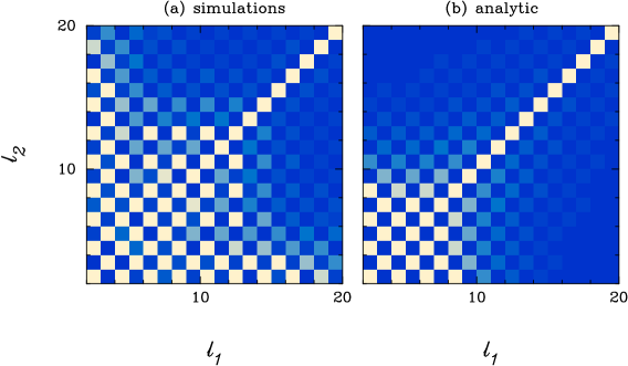
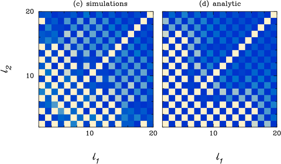
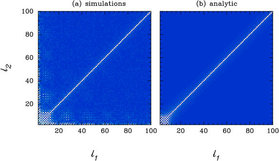
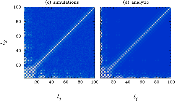
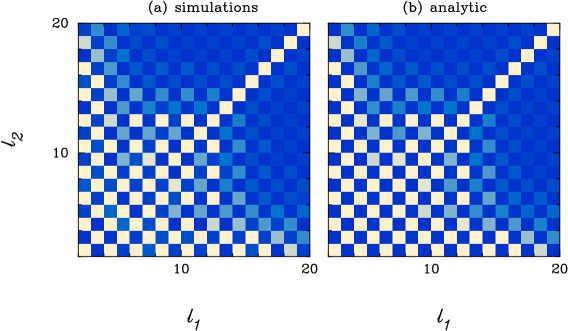
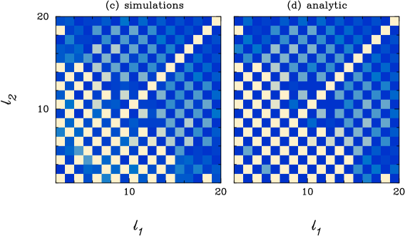
Figure 2 compares the covariance matrices determined from the simulations described in Section 2.1 (left hand panels) with the analytic expressions of equations (15a) and (17). For a Galactic cut of $\pm 10^{\circ}$, the analytic approximations are accurate at $\ell\lower 2.15277pt\hbox{$\;\buildrel>\over{\sim}\;$}20$, where the covariance matrix is very nearly band-diagonal, but fail at lower multipoles. At $\ell\lower 2.15277pt\hbox{$\;\buildrel<\over{\sim}\;$}20$, even the diagonal components of the analytic covariance matrices differ (by up to 25% at $\ell=2$) from the covariance matrices determined from the simulations (see Figure 12 of Section 5.4). The off-diagonal components differ by much larger factors and so the analytic approximations at low multipoles are useless for any quantitative application such as parameter estimation.

This can be seen in Figure 3, which shows a similar comparison to that shown in Figure 2, but using $2\times 10^{5}$ low resolution simulations with pixel size $\theta_{c}=5^{\circ}$ and Gaussian beam FWHM of $7^{\circ}$. However, for such a low resolution map, it is possible to evaluate an exact expression for the covariance matrix. This can be done conveniently by computing

$$\langle\Delta\tilde{C}^{p}_{\ell}\Delta\tilde{C}^{p}_{\ell^{\prime}}\rangle={2\over(2\ell+1)(2\ell^{\prime}+1)}\sum_{mm^{\prime}}|B_{\ell m\ell^{\prime}m^{\prime}}|^{2},$$ (18)

where $B_{\ell m\ell^{\prime}m^{\prime}}$ is evaluated by summing over pixels

$$B_{\ell m\ell^{\prime}m^{\prime}}=\sum_{ij}w_{i}w_{j}\Omega_{i}\Omega_{j}C(\theta_{ij})Y_{\ell m}({\bf\theta}_{i})Y^{*}_{{\ell^{\prime}}m^{\prime}}({\bf\theta}_{j}).$$ (19)

In equation (19), $C(\theta)$ is the temperature autocorrelation function

$$C(\theta_{ij})=\langle\Delta T_{i}\Delta T_{j}\rangle={1\over 4\pi}\sum_{\ell}(2\ell+1)C_{\ell}P_{\ell}(\cos\theta).$$ (20)

A comparison of the simulations with the exact expression (18) is shown in Figure 4. As expected, the agreement is almost perfect and any residual differences are simply caused by noise from the finite number of simulations.

Figure 4: As Figure 3, but now comparing with the exact expression for the covariance matrices (equation 18).

The procedure for estimating an accurate covariance matrix for a PCL estimator is therefore as follows:

(i) Adopt a (smooth) theoretical model for the power spectrum $C_{\ell}$. (This can be done iteratively, with an intermediate parameter estimation step if required).

(ii) Compute the covariance matrix for PCL estimates from the full resolution map using the approximate expression (15a).

(iii) Use the exact expression (18) to compute the covariance matrix at low multipoles by summation using a lower resolution pixelization.

(iv) Replace the elements of the covariance matrices at low multipoles ($\ell_{1}\leq\ell_{\rm J}$, $\ell_{2}\leq\ell_{\rm J}$) computed in step (ii) with the elements computed in step (iii).

There are a number of subtleties involved in this procedure. For example, what resolution should be used in step (iii)? How does one choose the ‘joining’ multipole $\ell_{\rm J}$ in step (iv)? What should one use for the final covariance matrix in the ranges ($\ell_{1}\leq\ell_{\rm J}$, $\ell_{2}>\ell_{\rm J}$) and ($\ell_{2}\leq\ell_{\rm J}$, $\ell_{1}>\ell_{\rm J}$) which are not computed in step (iii)? In the example discussed in Section (4), the joining multipole $\ell_{J}$ is simply chosen by trial and error so that the covariances matrices computed in steps (ii) and (iv) agree to high accuracy (a few percent or better). The components of the covariance matrices at ($\ell_{1}\leq\ell_{\rm J}$, $\ell_{2}>\ell_{\rm J}$) and ($\ell_{2}\leq\ell_{\rm J}$, $\ell_{1}>\ell_{\rm J}$) are simply retained, but their values are so low that for most purposes it would make no difference if these values were set to zero. None of these subtleties are critical, and the method is so fast that many choices can be explored to assess the accuracy of the method. As long as the sky cut is not too large, the method described here can return a deconvolved PCL estimate $\hat{C}^{p}_{\ell}$, together with an accurate covariance matrix. If the sky cut is large, then the method can return a PCL estimate $\tilde{C}^{p}_{\ell}$ (or ‘regularised’ estimate, equation (13)) together with an accurate covariance matrix. Including uncorrelated instrumental noise poses no fundamental problems, and is discussed in Section 5.

3 Maximum likelihood Estimation

3.1 NRML Estimators

In the NRML method (Bond et al., 1998) a set of parameters $a_{p}$, which may be estimates of the power spectrum $C_{\ell}$, is determined from the likelihood function (1) by Newton-Raphson iteration. First, guess a set of values for the parameters $a_{p}$ and then refine these by adding a correction

$$\delta a_{p}=\sum_{p^{\prime}}\ F_{pp^{\prime}}^{-1}{1\over 2}{\rm Tr}\left[\left(xx^{T}-C\right)\left(C^{-1}{\partial C\over\partial a_{p}}C^{-1}\right)\right],$$ (21a)

where $F$ (the Fisher matrix) is the expectation value of the curvature matrix

$$F_{pp^{\prime}}=-\left\langle{\partial^{2}{\cal L}\over\partial a_{p}\partial a_{p^{\prime}}}\right\rangle={1\over 2}{\rm Tr}\left[C^{-1}{\partial C\over\partial a_{p}}C^{-1}{\partial C\over\partial a_{p^{\prime}}}\right].$$ (21b)

This leads to a new set of values $a_{p}$ and the computation can be repeated until the estimates $a_{p}$ converge. An estimate of the covariance matrix for the parameters $a_{p}$ is given by the inverse of the Fisher matrix at the final iteration

$$\langle\delta a_{p}\delta a_{p^{\prime}}\rangle=F_{pp^{\prime}}^{-1}.$$ (22)

An alternative, and computationally more expensive NRML method uses the full curvature matrix instead of $F$ in equation (21a) (Borrill 1999b). The NRML estimator has been used widely in the analysis of CMB experiments, for example, MAXIMA-1 (Hanany et al., 2000), BOOMERANG (de Bernardis et al., 2000), WMAP (Hinshaw et al., 2003) and to galaxy clustering (Efstathiou and Moody 2001).

There are, however, some disadvantages in using the NRML method. If the method is to be used to estimate power spectra from a map with a large sky cut, the Fisher matrix $F_{\ell\ell^{\prime}}$ will be numerically singular (i.e. will have a high condition number, see Press et al., 1992). In this case, the iterations (21a) will not converge. This problem can be overcome by solving for band-power averages of the $C_{\ell}$ (Bond et al., 1998). However, band-power averaging involves a loss of information and can produce biases in the final estimates of the power spectra, depending on the choice of bands. Cosmological parameters are often estimated from the power spectrum estimates, $C^{e}_{\ell}$, by minimising a $\chi^{2}$,

$$\chi^{2}(q_{p})=\sum_{\ell\ell^{\prime}}(C^{T}_{\ell}(q_{p})-C^{e}_{\ell})F_{\ell\ell^{\prime}}(C^{T}_{\ell^{\prime}}(q_{p})-C^{e}_{\ell^{\prime}}),$$ (23)

with respect to the parameters $q_{p}$, where $C^{T}_{\ell}$ is the theoretical power spectrum. If the Fisher matrix (21b) is used in equation (23) then the parameters $q_{p}$ will be biased (Bond et al. 1998; Oh et al. 1999). This is because a low estimated value of $C^{e}_{\ell}$ will be assigned a low variance. This problem can be partially alleviated by smoothing the final estimates $C^{e}_{\ell}$ and re-computing the Fisher matrix (Oh et al. 1999). However, it is easy to think of cases where such a procedure would fail catastrophically, for example, for the low quadrupole amplitude measured by WMAP (Bennett et al. 2003). To avoid bias, what is wanted in equation (23) is the Fisher matrix appropriate to the estimator for the theoretical model of interest, i.e. $F_{\ell\ell^{\prime}}(C^{T}_{\ell})$, and preferably an accurate model of the likelihood function rather than the simple $\chi^{2}$ of equation (23). Clearly, it is not feasible to evaluate equation (21b) for every set of physical parameters $q_{p}$. One solution is to find a model for $F_{\ell\ell^{\prime}}$ which can be rescaled (or recallibrated) to a good approximation for any given theoretical model (see e.g. Verde et al. 2003). This approach is, in part, motivation for the hybrid estimator developed in Sections 4 and 5. For another approach to this problem, see Gupta and Heavens 2002).

Finally, since the NRML method iterates to a ML solution, the final estimates of $C^{e}_{\ell}$ are not easily expressible in terms of the data vector ${\bf x}$. In contrast, the QML estimator discussed in the next Section, as its name implies, is expressible in terms of products $x_{i}x_{j}$ of the data vector. This property is critical in defining the hybrid estimator of Sections 4 and 5.

3.2 QML Estimators

QML estimators have been used extensively by Tegmark and collaborators (e.g. Tegmark et al. 1998; Hamilton, Tegmark and Padmanabhan, 2000; Tegmark et al. 2002a; Tegmark, Hamilton and Xu, 2002b). Most other authors have used the NRML methods described in the previous sub-section, giving the impression that QML estimators are in some sense inferior to NRML estimators. One of the purposes of this sub-section is to show that this is impression is unjustified. As in previous Sections, instrumental noise is ignored to simplify the discussion. Instrumental noise is discussed in Section 5.2.

If the data vector $x_{i}$ is composed of Gaussian random variates, a minimum variance quadratic estimator of the power spectrum is

$$y_{\ell}=x_{i}x_{j}E^{\ell}_{ij},$$ (24a)

where

$$E^{\ell}={1\over 2}C^{-1}{\partial C\over\partial C_{\ell}}C^{-1}.$$ (24b)

(Tegmark 1997). Evidently, a functional form for $C_{\ell}$ ($C^{\rm in}_{\ell}$) must be assumed to compute the matrix (24b). However, the expectation value of $y_{\ell}$ provides an unbiased estimator of the true $C_{\ell}$ whatever the assumed form for $C^{\rm in}_{\ell}$,

$$\langle y_{\ell}\rangle=F_{\ell\ell^{\prime}}C_{\ell^{\prime}},$$ (25)

where $F_{\ell\ell^{\prime}}$ is the Fisher matrix of equation (21b) with $a_{p}$ replaced by $C_{\ell}$. As it stands, the vector $y_{\ell}$ will (usually) look very different to the power spectrum. However, we can recover an estimate that has a similar shape to the true power spectrum simply by rescaling

$$\tilde{C}^{q}_{\ell}=y_{\ell}/\sum_{\ell^{\prime}}F_{\ell\ell^{\prime}}.$$ (26)

The covariance matrix for the estimates $y_{\ell}$ is

$$\langle y_{\ell}y_{\ell^{\prime}}\rangle-\langle y_{\ell}\rangle\langle y_{\ell^{\prime}}\rangle=2{\rm Tr}\left[CE^{\ell}CE^{\ell^{\prime}}\right],$$ (27)

where the $C$’s appearing in equation (27) are the true covariance matrices. If the assumed form of $C_{\ell}$ is a good approximation to the true power spectrum, then equation (27) simplifies to

$$\langle\Delta y_{\ell}\Delta y_{\ell^{\prime}}\rangle=F_{\ell\ell^{\prime}}.$$ (28)

To summarise, if the initial guess is a poor approximation to the true $C_{\ell}$, equation (25) provides an unbiased estimate of the power spectrum provided that the guess for $C_{\ell}$ is used to compute the covariance matrices in the expressions for $E$ and $F$ (equations (24b) and (21b)). If the initial guess for $C_{\ell}$ is poor, the resulting estimates $y_{\ell}$, although providing unbiased estimates of $C_{\ell}$, will not be the ML solution and their covariances will be given by equation (27); the errors on the QML estimates, although accurate, will not be as small as those of a ML solution. If the initial guess for $C_{\ell}$ is close to the true answer, then the estimates of $y_{\ell}$ will be close to the ML solution and their covariances will be given accurately by equation (28). In practice, finding an acceptable initial guess for $C_{\ell}$ is unlikely to be a problem since the QML estimates at low multipoles are almost independent of the initial guess (see Section 3.3) and the CMB power spectrum at intermediate multipoles is already well estimated from WMAP. Henceforth we will assume that the initial guess for $C_{\ell}$ is close enough to the true answer that equation (28) applies.

If the Fisher matrix is non-singular (as is the case for a narrow Galactic cut) then equation (25) can be inverted to provide an unbiased QML estimate of $C_{\ell}$,

$$\hat{C}^{q}_{\ell}=F^{-1}_{\ell\ell^{\prime}}y_{\ell^{\prime}},$$ (29)

with covariance matrix

$$\langle\Delta\hat{C}^{q}_{\ell}\Delta\hat{C}^{q}_{\ell^{\prime}}\rangle=F^{-1}_{\ell\ell^{\prime}}.$$ (30)

The matrix $F$ is therefore an approximation to the Fisher matrix for the estimates $\hat{C}^{q}_{\ell}$.

With this formulation, there is a close analogy between the PCL estimates $\tilde{C}^{p}_{\ell}$ and $\hat{C}^{p}_{\ell}$ (equations (8) and (12)) and the QML estimates $\tilde{C}^{q}_{\ell}$ and $\hat{C}^{q}_{\ell}$ (eqations (26) and (29)). Both of the estimates $\tilde{C}^{p}_{\ell}$ and $\tilde{C}^{q}_{\ell}$ are related to the true power spectrum by convolutions. If a narrow Galactic cut is used, then these estimates can be deconvolved to form $\hat{C}^{p}_{\ell}$ and $\hat{C}^{q}_{\ell}$. However, this deconvolution step is not essential, since $\tilde{C}^{p}_{\ell}$ and $\tilde{C}^{q}_{\ell}$ contain the same information as the deconvolved estimates $\hat{C}^{p}_{\ell}$ and $\hat{C}^{q}_{\ell}$.

3.3 Fisher matrix for low multipoles

Suppose that the data vector $x_{i}$ consists of the spherical harmonic coefficients $\tilde{a}_{\ell m}$ measured on the cut sky. These coefficients are related to the true harmonic coefficients by the coupling matrix $K_{{\ell m}{\ell^{\prime}m^{\prime}}}$ (equation 5a). As discussed in Section 2.1, on a cut sky some combinations of the $a_{\ell m}$ define ‘null modes’ that lie within the cut and hence the matrix $K$ will be singular. However, if the Galactic cut is relatively narrow, the coefficients $\tilde{a}_{\ell m}$ at low multipoles will be weakly correlated with any of the $a_{\ell m}$ that define ‘null modes’ (Figure 2). In this case, the expansion (5a) can be truncated at finite ($\ell,m$) and ($\ell^{\prime},m^{\prime}$), and the truncated matrix $\tilde{K}$ for the cut sky can be inverted. (The invertibility of $\tilde{K}$ can be used to construct orthogonal functions on the cut sky from the spherical harmonics $Y_{\ell m}$, Górski 1994, Mortlock et al. 2002).

If $\tilde{K}$ is invertible, then we can reconstruct the approximations to the actual $a_{\ell m}$ coefficients on the uncut sky by performing the matrix inversion $a\approx\tilde{K}^{-1}\tilde{a}$. The QML estimates of $C_{\ell}$ (in the absence of instrumental noise) then reduce to

$$\hat{C}^{q}_{\ell}={1\over(2\ell+1)}\sum_{m}|a_{\ell m}|^{2}.$$ (31)

and so return almost the exact value of $C_{\ell}$ for our particular realization of the CMB sky in the presence of a Galactic cut (see also Efstathiou 2004). The Fisher matrix for the QML estimates is therefore simply

$$F_{\ell\ell^{\prime}}={(2\ell+1)\over 2C_{\ell}^{2}}\delta_{\ell\ell^{\prime}},$$ (32)

reflecting cosmic variance. In other words, the QML estimates $\hat{C}^{q}_{\ell}$ give cosmic variance limited estimates of the power spectrum independent of the size of a Galactic cut, provided that the cut is not too large. (For example, equation (32) is a good approximation at low multipoles for the Kp2 sky cut defined by the WMAP team but begins to break down for the Kp0 and larger sky cuts, see Efstathiou 2004). The usual formula

$$\langle\Delta C_{\ell}^{2}\rangle={2C^{2}_{\ell}\over(2\ell+1)f_{\rm sky}},$$ (33)

(e.g. Knox 1995) where $f_{\rm sky}$ is the fraction of the sky sampled by the experiment, clearly does not apply at low multipoles and one can think of the $f_{\rm sky}$ factor in (33) as reflecting the loss of information at high multipoles from the missing ‘null modes’ that lie within the Galactic cut.

Figure 5: The figure to the left shows the covariance matrix for the quadratic estimator $\hat{C}^{q}_{\ell}$ (equation 29) computed from $2\times 10^{5}$ simulations. The figure to the right shows the inverse of the Fisher matrix (equation 30).

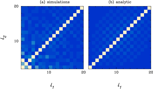
The results of this subsection are borne-out by a set of $2\times 10^{5}$ numerical simulations. In these simulations we apply the quadratic estimator (24a) to the same set of simulations used to construct Figures 3 and 4, using the pixel $\Delta T_{i}$ values as the data vector $x_{i}$. Figure 5 shows the resulting covariance matrix for the estimates $\hat{C}^{q}_{\ell}$ compared to the inverse of the Fisher matrix. There is some low-amplitude off-diagonal structure in both of the plots (as a consequence of the small coupling with ‘null modes’) but this is small and negligible for most purposes. The results from the simulations agree with equation (32) to within a few percent at multipoles $\ell\lower 2.15277pt\hbox{$\;\buildrel<\over{\sim}\;$}5$) and rise smoothly to match approximately with equation (33) by $\ell=30$ (see also Figure 14a below). Note that for the simulations used here, $f_{\rm sky}=0.83$. The discrepancy between the analytic and simulation results at low $\ell$ in Figure 5 is simply a consequence of the finite number of simulations. The off-diagonal elements of the covariance matrix estimated from the simulations at low multipoles are small compared to the diagonal elements (note that the grey-scale in Figures 2-5 was chosen to accentuate small amplitude structure) and become smaller as the number of simulations is increased.

Figure 6: The figure to the left shows the quadrupole amplitude estimated from the PCL estimator (ordinate) plotted against the quadrupole amplitude of the simulation used to generate the map (abscissa). (Points for 1000 simulations are shown). The figure to the right shows the equivalent plot for the QML estimator. The error bar in Figure (6a) shows the cosmic variance error for the mean value of $(\Delta T_{2})^{2}=1123\;(\mu{\rm K})^{2}$ for the input simulations.

The behaviour of the QML estimator differs from the PCL estimates $\hat{C}^{p}_{\ell}$, which are highly correlated at low multipoles (e.g. Figure 4) and which have a variance that significantly exceeds cosmic variance. As an example, Figure 6 compares the amplitudes of the quadrupole estimates, expressed as

$$(\Delta T_{\ell})^{2}={1\over 2\pi}\ell(\ell+1)C_{\ell},$$ (34)

compared to the input quadrupole amplitude in each simulation. The expectation value of the quadrupole amplitude for the simulations is $(\Delta T_{2})^{2}=1123\;(\mu{\rm K})^{2}$ (after smoothing with the Gaussian beam function) and so the cosmic variance is expected to lead to a dispersion of $710\;(\mu{\rm K})^{2}$. Figure 6, shows that the ‘estimator induced’ dispersion in the PCL case ($262\;(\mu{\rm K})^{2}$) is a significant fraction of the cosmic variance . For the QML case, the ‘estimator induced’ dispersion is much smaller ($68\;(\mu{\rm K})^{2}$). These numbers depend on the size of the Galactic cut, but it is clear that for realistic Galactic cuts the QML estimator returns amplitudes for low multipoles that are close to the true values for our particular realisation in the sky. This can be important, e.g. the WMAP quadrupole estimated using a PCL estimator has an amplitude of only $(\Delta T_{2})^{2}=123\;(\mu{\rm K})^{2}$, much smaller than the amplitude expected in the concordance $\Lambda$CDM cosmology (Bennett et al. 2003; Spergel et al. 2003). In contrast, the QML estimator applied to the WMAP internal linear combination map gives a quadrupole amplitude closer to $200\;(\mu{\rm K})^{2}$ (Efstathiou 2004).

3.4 Fisher matrix at high multipoles

In the pixel domain, the signal covariance matrix is

$$S_{ij}=\sum_{\ell}{(2\ell+1)\over 4\pi}w_{i}w_{j}C_{\ell}P_{\ell}(\theta_{ij})=\sum_{\ell m}C_{\ell}w_{i}w_{j}Y_{\ell m}({\bf\theta}_{i})Y^{*}_{\ell m}({\bf\theta}_{j}),$$ (35)

where $w_{i}$ is the (arbitrary) pixel weight function introduced in equation (3). If the data cover the whole sky (and the weight function $w_{i}$ is everywhere non-zero), then from the orthogonality of the spherical harmonics, the inverse signal covariance matrix is given by

$$S_{ij}^{-1}=\sum_{\ell m}{\Omega_{i}\Omega_{j}\over C_{\ell}w_{i}w_{j}}Y^{*}_{\ell m}({\bf\theta}_{i})Y_{\ell m}({\bf\theta}_{j}).$$ (36)

Although equation (36) applies strictly only for the complete sky, it will be a good approximation for a cut sky with $i$ and $j$ restricted to the pixels outside the cut, provided that the total number of pixels in the map is very much greater than the number of pixels close to the boundary. (This condition is satisfied in all of the examples discussed in this paper). The product $C^{-1}\partial C/\partial C_{\ell}$ in (24b) is then

$$S_{ij}^{-1}{\partial S_{jk}\over\partial C_{\ell}} = \sum_{j}\sum_{m\ell_{1}m_{1}}{\Omega_{j}\Omega_{j}\over C_{\ell_{1}}w_{i}w_{j}}Y_{\ell_{1}m_{1}}(\theta_{i})Y^{*}_{\ell_{1}m_{1}}(\theta_{j})\;w_{j}w_{k}Y_{\ell m}(\theta_{j})Y^{*}_{\ell m}(\theta_{k})$$ (37)

$$\approx {1\over C_{\ell}}\sum_{m}\Omega_{i}{w_{k}\over w_{i}}Y_{\ell m}(\theta_{i})Y^{*}_{\ell m}(\theta_{k}).$$

The Fisher matrix (21b) is therefore

$$F_{\ell\ell^{\prime}}\approx{1\over 2C_{\ell}C_{\ell^{\prime}}}\sum_{ik}\sum_{mm^{\prime}}\Omega_{i}\Omega_{k}Y_{\ell m}(\theta_{i})Y^{*}_{\ell m}(\theta_{k})Y_{\ell^{\prime}m^{\prime}}(\theta_{k})Y^{*}_{\ell^{\prime}m^{\prime}}(\theta_{i}).$$ (38)

Notice that weight factors $w_{i}$ have cancelled and do not appear in equation (38). This is what is expected; if the data vector $x_{i}$ is multiplied by arbitrary weights and a maximum likelihood estimator applied to estimate $C_{\ell}$, then neither the estimates $\hat{C}^{q}_{\ell}$ nor their covariance matrix should depend on the weights. The derivation leading to equation (38) differs from that in Appendix D.1.2 of Hinshaw et al. (2003) which assumes equal weight per pixel. The final answer does, however, agree with equation (D19) of Hinshaw et al. (2003).

Evaluating the summations in equation (38), we find

$$F_{\ell\ell^{\prime}}\approx{(2\ell+1)(2\ell^{\prime}+1)\over 2C_{\ell}C_{\ell^{\prime}}}G_{\ell\ell^{\prime}}={(2\ell+1)\over 2C_{\ell}C_{\ell^{\prime}}}M_{\ell\ell^{\prime}},$$ (39)

where the matrices $G_{\ell\ell^{\prime}}$ and $M_{\ell\ell^{\prime}}$ are the coupling matrices defined by equations (9) and (11) evaluated for unit weight per pixel over the uncut sky.

Notice that for high multipoles, equation (17) for the covariance matrix of the deconvolved PCL estimates is equal to

$$\langle\Delta\hat{C}^{p}_{\ell}\Delta\hat{C}^{p}_{\ell^{\prime}}\rangle\approx{2C_{\ell}C_{\ell^{\prime}}\over(2\ell+1)}M^{-1}_{\ell\ell^{\prime}},$$ (40)

which is equal to the inverse of equation (39). It therefore follows that: (i) in the signal dominated limit and (ii) for high multipoles ($\ell$ greater than the width of the window function $\tilde{W}_{\ell}$), the deconvolved PCL estimate with equal weight per pixel is optimal and statistically equivalent to a maximum-likelihood solution. In the signal-dominated limit, there is therefore nothing to be gained by solving the ${\cal O}(N_{d}^{3})$ computational problem to apply a ML method, since the much faster PCL estimate will give a result that is statistically equivalent.

4 Hybrid estimator

Figure 7: The upper figure shows a simulated CMB sky with smoothing $\theta_{s}=1^{\circ}$ pixelized into $0.5^{\circ}\times 0.5^{\circ}$ pixels using an ‘igloo’ type pixelization scheme ($164828$ pixels in total). The lower figure shows the same map smoothed to $\theta_{s}=5^{\circ}$ and pixelized into $1632$ pixels of area $5^{\circ}\times 5^{\circ}$.

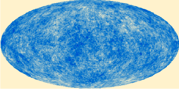
Having established that the PCL estimator is very close to optimal at high multipoles, it is clear that a fast and almost optimal power spectrum estimate can be derived by combining a PCL estimate with a QML estimate applied to a degraded low resolution map. As an example, consider the maps shown in Figure 7. The map in the upper panel is one of the simulations used for the tests described in Section 2.1 (pixel size $\theta_{c}=0.5^{\circ}$, $\theta_{s}=1^{\circ}$). The map in the lower panel was constructed from the same $a_{\ell m}$ coefficients with pixel size $\theta_{c}=5^{\circ}$ and smoothed to $\theta_{s}=5^{\circ}$. Figure 7 plots the maps over the whole sky, but as in previous Sections a cut of $\pm 10^{\circ}$ above and below the notional Galactic plane has been applied in the tests described below. There are $1385$ active pixels outside Galactic cut in the low resolution map and so it takes only a few seconds to compute all of the ${\cal O}(N_{d}^{3})$ operations required for the QML estimator.

From these maps, two estimates of the power spectrum can be formed, $\hat{C}^{p}_{\ell}$ (up to a maximum multipole $\ell=\ell_{p}$) and $\hat{C}^{q}_{\ell}$ (up to maximum multipole $\ell=\ell_{q}$), together with accurate estimates of their covariance matrices, as discussed in previous Sections. The cross-correlation between the QML and PCL estimates at low multipoles is given by

$$\langle\Delta\tilde{C}^{p}_{\ell}\Delta\hat{C}^{q}_{\ell^{\prime}}\rangle\approx{2C_{\ell^{\prime}}^{2}\over(2\ell^{\prime}+1)}M_{\ell\ell^{\prime}},\qquad\langle\Delta\hat{C}^{p}_{\ell}\Delta\hat{C}^{q}_{\ell^{\prime}}\rangle\approx{2C_{\ell^{\prime}}^{2}\over(2\ell^{\prime}+1)}\delta_{\ell\ell^{\prime}},$$ (41)

where we have assumed the approximate expression for the QML estimator of equation (31). Equation (41) has been used in the analysis described below and is a perfectly adequate approximation for $\ell\lower 2.15277pt\hbox{$\;\buildrel<\over{\sim}\;$}30$. If necessary, a more accurate expression for the cross-correlations can be evaluated from a sum over pixels, as in the analysis of the PCL covariance matrix described in Section 2.2:

$$\langle\Delta\tilde{C}^{p}_{\ell}\Delta y_{\ell^{\prime}}\rangle={2\over(2\ell+1)}\sum_{mpq}z_{plm}z^{*}_{qlm}E^{\ell^{\prime}}_{pq},$$ (42a)

where

$$z_{jlm}=\sum_{i}C(\theta_{ij})w_{i}\Omega_{i}Y_{\ell m}(\theta_{i}).$$ (42b)

Figure 8: The filled circles show the results of applying the QML estimator to the low resolution map shown in Figure 7. The error bars are computed from the diagonal components of the inverse of the Fisher matrix (equation 21b). Three rows of the Fisher matrix are shown in the panels to the right. The stars show the deconvolved PCL estimates $\hat{C}^{p}_{\ell}$ determined from the high resolution map shown in Figure 7. The dotted line shows the fiducial $\Lambda$CDM power spectrum and the solid line shows the actual power spectrum computed from the $a_{\ell m}$ coefficients used to generate the maps. A sky cut of $\pm 10^{\circ}$ has been used for the estimated power spectra and the QML estimates have been corrected to a beam smoothing of $1^{\circ}$ as used in the high resolution maps.

Given expressions for the covariances and the cross-covariances, we can combine the two estimates $\hat{C}^{q}_{\ell}$ and $\hat{C}^{p}_{\ell}$ into a single data vector $\hat{C}_{\alpha\ell}$ ($\alpha\equiv q,p)$ and form the $\chi^{2}$

$$\chi^{2}=(\hat{C}_{\alpha\ell_{1}}-\hat{C}^{h}_{\ell_{1}}){\cal F}_{\alpha\ell_{1}\beta\ell_{2}}(\hat{C}_{\beta\ell_{2}}-\hat{C}^{h}_{\ell_{2}}),$$ (43)

where ${\cal F}_{\alpha\ell_{1}\beta\ell_{2}}$ is the inverse of the covariance matrix $\langle\Delta\hat{C}_{\alpha\ell_{1}}\Delta\hat{C}_{\beta\ell_{2}}\rangle$. Minimising equation (43) gives the solution for the hybrid estimate $\hat{C}^{h}_{\ell}$

$$\sum_{\alpha\beta\ell_{1}}{\cal F}_{\alpha\ell_{1}\beta\ell}\hat{C}^{h}_{\ell_{1}}=\sum_{\alpha\beta\ell_{1}}{\cal F}_{\alpha\ell_{1}\beta\ell}\hat{C}_{\alpha\ell_{1}},$$ (44)

with covariance matrix

$$\langle\Delta\hat{C}^{h}_{\ell_{1}}\Delta\hat{C}^{h}_{\ell_{2}}\rangle=\left(\sum_{\alpha\beta}{\cal F}_{\alpha\ell_{1}\beta\ell_{2}}\right)^{-1}.$$ (45)

The hybrid estimator $\hat{C}^{h}_{\ell}$ therefore makes a smooth transition between the QML estimates at low multipoles and the PCL estimates at high multipoles (and would be exactly equal to the quadratic estimates at low multipoles if the Fisher matrix were precisely diagonal). From the results presented in Sections 2.2 and 3.2, the covariance matrix for the hybrid estimates (45) is expected to be predominently band-diagonal at all multipoles if the sky cut is relatively narrow. Furthermore, since each of the estimates $\hat{C}^{q}_{\ell}$ and $\hat{C}^{p}_{\ell}$ is an unbiased estimate of $C_{\ell}$, it follows from equation (44) that the hybrid estimator $\hat{C}^{h}_{\ell}$ is unbiased.

Figure 9: The filled circles show the hybrid estimates $\hat{C}^{h}_{\ell}$ for the maps shown in Figure 7 computed from equation (44). The error bars were computed from diagonal components of the covariance matrix (45). As in Figure 8, the dotted line shows the fiducial $\Lambda$CDM power spectrum and the solid line shows the actual power spectrum computed from the $a_{\ell m}$ coefficients used to generate the maps.

Figure 10: The left hand panel shows the analytic covariance matrix at $\ell\leq 50$ for the PCL estimates. The right hand panel shows the covariance matrix for the hybrid estimates $\hat{C}^{h}_{\ell}$ computed from equation (45).

To illustrate the hybrid method, Figure 8 shows a comparison of the QML and PCL estimates at low multipoles derived from the maps shown in Figure 7. Three rows of the Fisher matrix for the QML estimates are shown in the panels to the right. As expected, for a sky cut of $\pm 10^{\circ}$, the QML Fisher matrix is almost exactly diagonal at low multipoles and so the estimates $\hat{C}^{q}_{\ell}$ agree almost perfectly with the power spectrum computed from the $a_{\ell m}$ for this particular simulation. By multipoles $\ell\approx 10$ the QML and PCL estimates become similar.

The hybrid estimate computed from equation (44) are shown in Figure 9. In this example, the QML estimates were retained up to $\ell_{q}=20$. For the PCL estimator, the exact expression for the covariance matrix (equation 18) was used for $\ell\leq 20$ and the approximate expression (equation 15a) was used for higher multipoles. Neither of these choices are critical, as can be seen from the close agreement between QML and PCL estimates plotted in Figure 8.

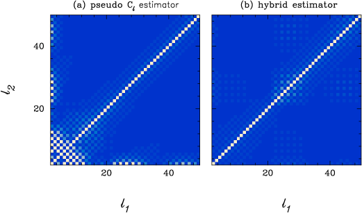
The analytic covariance matrices for the PCL estimator (cf Figure 2d) and the hybrid estimator (equation 45) are plotted in Figure 10 for multipoles $\ell\leq 50$. As expected, the covariance matrix for the hybrid estimator is almost band-diagonal. In Section 3.4 it was proved that the PCL estimator with equal weight per pixel is statistically equivalent to the QML estimator if instrumental noise can be neglected. The hybrid estimates plotted in Figure 9 should therefore be almost indistinguishable from a brute force ${\cal O}(N_{d}^{3})$ ML analysis of the high resolution map shown in Figure 7. However, in contrast to the ${\cal O}(N_{d}^{3})$ methods, computation of the hybrid estimator and its covariance matrix takes of order seconds on a laptop computer.

The analysis of the hybrid estimator, as described above, applies if the estimators $\hat{C}^{p}_{\ell}$ and $\hat{C}^{q}_{\ell}$ can be constructed from the estimates $\tilde{C}^{p}_{\ell}$ and $\tilde{C}^{q}_{\ell}$, i.e. if the Galactic cut is narrow enough. For a large Galactic cut, it may not be possible to contruct $\hat{C}^{p}_{\ell}$ and $\hat{C}^{q}_{\ell}$. In this case, one can simply use the hybrid $\chi^{2}$ of equation (43) to estimate cosmological parameters (or a suitably modified function to account for the deviations from Gaussianity at low multipoles) in place of the $\chi^{2}$ of equation (23). Or, equivalently, one can solve for a suitably regularized hybrid power spectrum, $R\hat{C}^{h}_{\ell}$, (equation 13) and its covariance matrix. There is no requirement to construct a deconvolved hybrid estimate $\hat{C}^{h}_{\ell}$ and no loss of information in working with a regularised estimate.

5 Including noise

Including uncorrelated noise poses no fundamental problems. In the first two subsections some of the formulae of the previous Sections are generalised, without detailed mathematical proof, to include uncorrelated noise. The motivation for applying a hybrid estimator to noisy data is given in Section 5.3, and an application to a high resolution simulation with a Planck-type scanning pattern is described in Section 5.4. For simplicity, we consider only the case of white noise in this Section, neglecting the $1/f$-type noise that is expected in a real experiment. Possible ways of handling $1/f$ noise are discussed briefly in Section 6.

5.1 PCL estimator including noise

If noise is included, the PCL estimator (7) has expectation value

$$\langle\tilde{C}^{p}_{\ell}\rangle=\sum_{\ell^{\prime}}C_{\ell^{\prime}}M_{\ell\ell^{\prime}}+\langle\tilde{N}_{\ell}\rangle,$$ (46)

(e.g. Hivon et al. 2002) where the noise power spectrum is, in general,

$$\tilde{N}_{\ell}={1\over 4\pi}\sum_{ij}N_{ij}w_{i}w_{j}\Omega_{i}\Omega_{j}P_{\ell}(\theta_{ij}).$$ (47)

If the noise matrix is diagonal, $N_{ij}=\sigma_{i}^{2}\delta_{ij}$, equation (47) simplifies to

$$\tilde{N}_{\ell}={1\over 4\pi}\sum_{i}\sigma_{i}^{2}w^{2}_{i}\Omega^{2}_{i}.$$ (48)

To form an unbiased PCL estimator of the power spectrum, then we simply subtract the noise term, $\tilde{C}^{\prime p}_{\ell}=\tilde{C}^{p}_{\ell}-\tilde{N}_{\ell}$, and compute the deconvolved estimates $\hat{C}^{p}_{\ell}=M^{-1}_{\ell\ell^{\prime}}\tilde{C}^{\prime p}_{\ell^{\prime}}$.

The covariance matrix of $\tilde{C}^{\prime p}_{\ell}$ is

$$\langle\Delta\tilde{C}^{\prime p}_{\ell}\Delta\tilde{C}^{\prime p}_{\ell^{\prime}}\rangle=\tilde{V}^{\prime}_{\ell\ell^{\prime}}=\tilde{V}_{\ell\ell^{\prime}}+\langle\Delta\tilde{C}^{N}_{\ell}\Delta\tilde{C}^{N}_{\ell^{\prime}}\rangle+\tilde{U}_{\ell\ell^{\prime}},$$ (49)

where $\tilde{V}_{\ell\ell^{\prime}}$ is given by equation (15a). The noise covariance in equation (49) is

$$\langle\Delta\tilde{C}^{N}_{\ell}\Delta\tilde{C}^{N}_{\ell^{\prime}}\rangle=2\Xi(\ell,\ell^{\prime},\tilde{W}^{N}),$$ (50a)

where

$$\tilde{W}^{N}_{\ell}={1\over(2\ell+1)}\sum_{m}|\tilde{w}^{N}_{\ell m}|^{2},\qquad w^{N}_{\ell m}=\sum_{i}\sigma_{i}^{2}w_{i}^{2}\Omega_{i}^{2}Y_{\ell m}(\theta_{i}),$$ (50b)

and the cross-covariance $\tilde{U}_{\ell\ell^{\prime}}$ is given by

$$\tilde{U}_{\ell\ell^{\prime}}=4(C_{\ell}C_{\ell^{\prime}})^{1/2}\Xi(\ell,\ell^{\prime},\tilde{W}^{SN}),$$ (51a)

where

$$\tilde{W}^{SN}_{\ell}={1\over(2\ell+1)}\sum_{m}{\it Re}(w^{(2)}_{\ell m}w^{*N}_{\ell m}).$$ (51b)

The covariance matrix of the deconvolved estimates including noise is

$$\langle\Delta\hat{C}^{p}_{\ell}\Delta\hat{C}^{p}_{\ell^{\prime}}\rangle=M^{-1}\tilde{V}^{\prime}(M^{-1})^{T},$$ (52)

with $M$ as given in equation (9). All of the results quoted in this Section have been derived under the assumption that the window functions are narrow compared to variations in $C_{\ell}$, and the factor $(C_{\ell}C_{\ell^{\prime}})^{1/2}$ in equation (51a) has been written in this way to preserve the symmetry of the matrix $\tilde{V}^{\prime}$. An equivalent result to equation (49) has been derived independently by Chon et al. (2003).

5.2 QML estimator including noise

For a general noise matrix $N_{ij}$, we can define an unbiased QML estimate by redefining $y_{\ell}$ equation (24a) as

$$y^{\prime}_{\ell}=x_{i}x_{j}E^{\ell}_{ij}-N_{ij}E^{\ell}_{ij},$$ (53)

(Tegmark 1997). The expectation value of $y^{\prime}_{\ell}$ is then given by equation (25) with the Fisher matrix as defined in equation (21b) where $C=S+N$. The covariance matrix of the estimates $y^{\prime}_{\ell}$ are given by equation (27).

If the noise matrix is diagonal and dominates over the signal, $C_{ij}\approx N_{ij}=\sigma_{i}^{2}\delta_{ij}$, then

$$E^{\ell}_{ij}\approx{(2\ell+1)\over 8\pi}{1\over\sigma_{i}^{2}\sigma_{j}^{2}}P_{\ell}(\theta_{ij}),$$ (54)

and the QML estimator is

$$2y_{\ell}=2x_{i}x_{j}E^{\ell}_{ij}=\sum_{mij}{x_{i}\over\sigma_{i}^{2}}{x_{j}\over\sigma_{j}^{2}}Y_{\ell m}(\theta_{i})Y^{*}_{\ell m}(\theta_{j})=(2\ell+1)\tilde{C}^{p}_{\ell},$$ (55)

where $\tilde{C}^{p}_{\ell}$ is the PCL estimate using a weight function $w_{i}=1/(\sigma^{2}_{i}\Omega_{i})$. In other words, if the noise dominates and is diagonal, the QML estimator is mathematically equivalent to a PCL estimate computed with inverse variance weighting. In this limit, the expectation value of the QML estimates $y^{\prime}_{\ell}$ is zero and their covariance matrix is

$$\langle\Delta y^{\prime}_{\ell_{1}}\Delta y^{\prime}_{\ell_{2}}\rangle=F_{\ell_{1}\ell_{2}}={(2\ell_{1}+1)(2\ell_{2}+1)\over 2}\Xi(\ell_{1},\ell_{2},\tilde{W}^{\sigma}),$$ (56a)

where

$$\tilde{W}^{\sigma}_{\ell}={1\over(2\ell+1)}|\tilde{w}^{\sigma}_{\ell m}|^{2},\qquad w^{\sigma}_{\ell m}=\sum_{i}{1\over\sigma_{i}^{2}}Y_{\ell m}(\theta_{i}).$$ (56b)

Equation (56a) agrees with equation (D12) of Hinshaw et al. (2003). The covariance matrix of the QML estimates $\hat{C}^{q}_{\ell}=F^{-1}_{\ell\ell^{\prime}}y^{\prime}_{\ell^{\prime}}$ is given by $F^{-1}$ as in equation (30) and is identical to the covariance matrix of equation (52) if the weight function is set to $w_{i}=1/(\sigma^{2}_{i}\Omega_{i})$. If the noise is the same in each pixel and each pixel has the same area ( $\sigma_{i}^{2}=\sigma^{2}_{p}$, $\Omega_{i}=\Omega_{p}$), then the diagonal components of equation (56a) give the usual approximate formula (e.g. Knox 1995)

$$\langle(\Delta\hat{C}^{q}_{\ell})^{2}\rangle\approx{2\over(2\ell+1)}{(\sigma^{2}_{p}\Omega_{p})^{2}\over f_{\rm sky}}.$$ (57)

5.3 Motivation for a hybrid estimator

The results presented above and in Sections 2 and 3 show that:

(I) in the signal dominated limit a PCL estimate with equal weight per pixel, $w_{i}=1$, is statistically equivalent to a ML estimate.

(II) in the noise dominated limit, and assuming that the noise matrix is diagonal, a PCL estimate with inverse variance weighting, $w_{i}=1/(\sigma_{i}^{2}\Omega_{i})$, is mathematically equivalent to a ML estimate.

For a realistic experiment such as WMAP, regime (I) is a good approximation at low multipoles and regime (II) is a good approximation at high multipoles, but in the intermediate regime it is difficult to derive a simple analytic formula for the optimal PCL weights. To do so, we would need an approximation to the inverse $C^{-1}=(S+N)^{-1}$, which appears in the Fisher matrix (equation 21b). In the harmonic domain $S$ is sparse while $N$ is not, but in the pixel domain $N$ is usually sparse while $S$ in not. Hence when $S$ and $N$ are comparable, the matrix $C$ is not sparse in either domain and so it is difficult to derive analytic approximations to $C^{-1}$. The non-sparseness of $C$ is the fundamental reason why it is difficult to solve the ${\cal O}(N_{d}^{3})$ problem in the numerical computation of ML estimators.

One solution, adopted by the WMAP team (Hinshaw et al. 2003), is to use a heuristic weighting in the intermediate regime. In the analysis of the WMAP data, Hinshaw et al. (2003) adopt equal weight per pixel at $\ell<200$, inverse variance weighting, $w_{i}=N_{\rm obs}(i)$ (where $N_{\rm obs}$ is the number of observations, or hit count, of pixel $i$) at $\ell>450$, and a heuristic weighting of

$$w_{i}={1\over 1/\langle N_{\rm obs}\rangle+1/N_{\rm obs}(i)},$$ (58)

in the intermediate range $200<\ell<450$, where $\langle N_{\rm obs}\rangle$ is the average hit count over the unmasked sky. This is a reasonable solution, but has the disadvantage that the final power spectrum and associated covariance matrix are contructed from three estimators with discontinuous joins at $\ell=200$ and $\ell=450$. It is worth mentioning here that if the noise matrix is assumed to be diagonal, the only benefit of solving the full ${\cal O}(N_{d}^{3})$ ML problem at high multipoles is to derive a continuous power spectrum estimate that is optimal in the intermediate regime.

The hybrid estimator discussed in Section 4 offers an alternative, but much faster, way of deriving a continuous power spectrum estimate between regimes (I) and (II), together with an accurate covariance matrix. Following Section 4, compute two PCL estimate $\hat{C}^{pw_{1}}_{\ell}$, and $\hat{C}^{pw_{2}}_{\ell}$, where the superscripts denote two different weight functions. The two PCL estimates can be combined with QML estimates at low multipoles to form a single data vector $\hat{C}_{\alpha\ell}$, where $\alpha\equiv q,pw_{1},pw_{2}$. Equations (44) and (45) can then be solved to give a hybrid estimate $\hat{C}^{h}_{\ell}$ and its associated covariance matrix. This requires the cross-covariance of the two PCL estimates, which is straightforward to derive following the analysis of Sections 2.2 and 5.1; simply replace the terms $w_{i}^{2}$ in equations (15b), (50b) and (51b) by the product $(w_{1})_{i}(w_{2})_{i}$.

If the weight function $(w_{1})_{i}$ is chosen to be equal weight per pixel, and weight function $(w_{2})_{i}$ is chosen to be $(w_{2})_{i}=1/(\sigma_{i}^{2}\Omega_{i})$, (or a suitably regularized weighting, see Section 5.4) then the hybrid estimate $\hat{C}^{h}_{\ell}$ will return answers that are a close approximation to the ML solution over the full range of multipoles. This method can be applied to any number of PCL estimates, for example, one could include a third PCL estimate with a heuristic intermediate weighting as in equation (58). In the examples described in Section 5.4 only two PCL estimates (equal weighting and a regularized inverse variance weighting) are used even though the the results would improve slightly by including an intermediate weighting scheme.

Our final procedure for estimating a power spectrum is therefore as follows:

(i) Compute a QML estimate from a low resolution map at low multipoles. If necessary, this estimate can include a general noise matrix $N_{ij}$.

(ii) Compute PCL estimates from a high resolution map using a number of weighting schemes, e.g. equal weight per pixel and inverse variance weighting.

(iii) Combine the estimates from steps (i) and (ii) together with their covariances and cross-covariances and solve for the hybrid estimate $\hat{C}^{h}_{\ell}$ and its covariance matrix as described in Section 4.

5.4 Numerical examples

Figure 11: Map showing the hit count distribution for a Planck-like scanning strategy in Galactic coordinates (see text for details). Darker regions close to the ecliptic poles have a higher hit count.

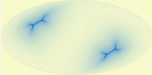
To illustrate the hybrid estimator in the presence of instrumental noise, we have simulated the hit count distribution for a Planck-type scanning strategy (Figure 11). In this example, the spin-axis of the spacecraft is aligned along the ecliptic plane, but a slow precession of $\theta=5^{\circ}\sin(2\phi_{e})$ is applied as the spacecraft scans in ecliptic longitude $\phi_{e}$. Figure 11 was constructed for a single detector, pointing at an angle of $85^{\circ}$ with respect to the spin-axis, and for a uniform scan rate in $\phi_{e}$. With this scanning geometry, the entire sky is scanned as $\phi_{e}$ varies from $0$ to $2\pi$ and the regions with high hit-count are concentrated at the ecliptic poles as shown in Figure 11. If the mean hit-count $\langle N_{\rm obs}\rangle$ is normalised to unity, the hit-count distribution in Figure 11 varies from a minimum of $0.54$ to a maximum of $120$.

Figure 12: The points show the square roots of the diagonal components of the covariance and cross-covariance, derived from $5\times 10^{4}$ simulations, of the deconvolved PCL estimates, divided by the simple formula of equation (59). The simulations have the same parameters as the high resolution map plotted in Figure 7 but include a uncorrelated noise for a Planck-type scanning pattern as shown in Figure 11 (see text for details). The results are shown for equal weight per pixel and for inverse variance weighting. The lines show the analytic model of equations (49) and (52).

Figure 13: The analytic covariance matrices for the deconvolved PCL estimates $\hat{C}^{p}_{\ell}$ compared with the results from $5\times 10^{4}$ simulations including noise. The upper panel (figures 13a and 13b) shows the covariance matrices for equal weight per pixel. The middle panel (figures 13c and 13d) shows the covariance matrices for inverse variance weighting. The lower panel (figures 13e and 13f) shows the cross-covariance between the estimates for these two weighting schemes.

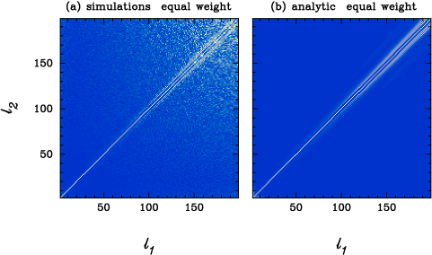
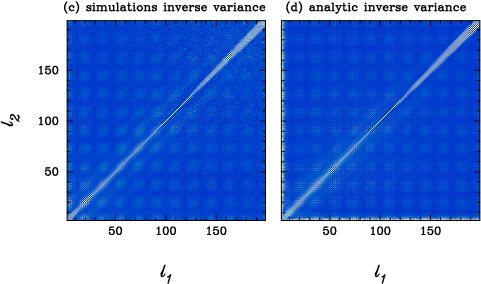
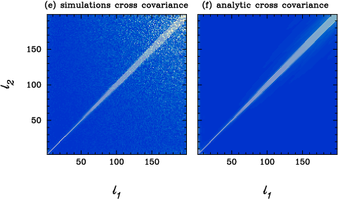
Figure 12 compares the diagonal components of the covariance and cross-covariance matrices for deconvolved PCL estimates, $\hat{C}^{p}_{\ell}$, for a set of $5\times 10^{4}$ simulations against the analytic formulae given in Section 5.1. The simulations have the same parameters as the high resolution map shown in Figure 7 ($\theta_{c}=0.5^{\circ}$, $\theta_{s}=1^{\circ}$) and the noise level was normalized to $\sigma_{p}=1\times 10^{-4}$ for pixels with the mean hit count. As in previous Sections a Galactic cut of $\pm 10^{\circ}$ was imposed. The filled circles in Figure 12 shows the square roots of the diagonal components of the covariance and cross-covariance matrices divided by the approximate formula (Knox 1995)

$$\langle(\Delta\hat{C}_{\ell})^{2}\rangle^{1/2}\approx\left({2\over(2\ell+1)f_{\rm sky}}\right)^{1/2}(C_{\ell}+\sigma^{2}_{p}\Omega_{p}).$$ (59)

As expected from the analysis of Section 5.1, inverse noise weighting leads to smaller errors than equal weighting at $\ell\lower 2.15277pt\hbox{$\;\buildrel>\over{\sim}\;$}100$ when the noise dominates the error budget. However, inverse variance weighting leads to much poorer estimates of the power spectrum at $\ell\lower 2.15277pt\hbox{$\;\buildrel<\over{\sim}\;$}100$. This is caused by the cusp-like structure of the hit count distribution shown in Figure 11. For this scanning pattern, the small number of pixels with a high hit counts close to the ecliptic poles dominate the PCL estimates with inverse variance weighting, consequently the errors on the PCL estimates at low multipoles are much larger than expected from cosmic variance. This scanning strategy was chosen intentionally to illustrate the differences between inverse variance weights and equal weights. The differences between these weighting schemes would be smaller for a WMAP-like scanning strategy, which produces a smooth variation of the hit counts with ecliptic latitude.

Figure 14: Figure 14a shows the analytic dispersions, normalized by equation (59), for various weighting schemes. These have been computed for a map with $0.1^{\circ}$ pixels, a smoothing of $\theta_{s}=0.2^{\circ}$, and a Planck-type noise pattern as shown in Figure 11. The noise level was set to $\sigma_{p}=2\times 10^{-5}$ for a pixel with the average hit count. The parameter $\epsilon_{f}$ is the regularizing parameter in the weighting scheme of equation (60). The dashed line in Figure 14a was computed from the diagonal components of the covariance matrix for the hybrid estimator (equation 45) applied to a data vector consisting of QML estimates over the range $2\leq\ell\leq 40$, PCL estimates with equal weight per pixel over the range $2\leq\ell\leq 1000$, and PCL estimates with $\epsilon_{f}=0.5$ weighting over the range $500\leq\ell\leq 1000$. Figures (b)-(d) show the PCL estimates for the same simulation for three different weighting schemes. The solid line shows the power spectrum for this particular simulation and the dotted line shows the power spectrum of the fiducial $\Lambda$CDM model. The power spectra in these figures have been corrected to zero beam width. Note that the abscissae in all of these plots uses a mixed logarithmic-linear scale in $\ell$, so that the behaviour of the power spectrum at low multipoles is clearly visible; the scale is logarithmic over the rangle $2\leq\ell\leq 20$ and linear at higher multipoles.

Another consequence of the cuspiness of the hit count distribution of Figure 11 is that the window function $\tilde{W}^{(2)}$ (equation (15b) for inverse variance weighting is broader the window function for equal weights. For inverse variance weighting, the analytic approximation to the covariance matrix $\tilde{V}_{\ell\ell^{\prime}}$ is therefore not as accurate at low multipoles as it is for equal weights. The full matrices are compared with the analytic formulae in Figure 13. As expected, the analytic formulae are in excellent agreement with the results from the simulations at high multipoles. However, there are large discrepancies at low multipoles in the case of inverse variance weighting that are clearly visible in Figures 13c and 13d. As described in Section 2.2, the covariance matrices (and cross-covariances) at low multipoles can be evaluated accurately by summing over pixels using degraded resolution maps (cf equation 18), but as we will see in the next example, there is no need to compute these components for the hybrid estimator.

As a final illustration of the hybrid estimator, we have analysed a simulation with $0.1^{\circ}$ pixels and a beam smoothing of $\theta_{s}=0.2^{\circ}$. The simulated map contains $4.12\times 10^{6}$ pixels and is therefore comparable in size and resolution to the CMB maps produced by WMAP. A Planck-like scanning strategy, as shown in Figure 11, was adopted and the noise level was set to $\sigma_{p}=2\times 10^{-5}$ for pixels with the mean hit count. At this resolution, the cuspiness in the hit count distribution causes numerical problems in evaluating the PCL esimator at high multipoles if exact inverse variance weighting is used. These can be avoided by introducing a regularising parameter $\epsilon_{f}$,

$$w_{i}={\sigma^{2}_{p}\langle\Omega_{i}\rangle\over(\sigma^{2}_{i}+\epsilon_{f}\sigma^{2}_{p})\Omega_{i}},$$ (60)

in the weight function (cf the heuristic weight function of equation (58)). The analytic dispersions for the deconvolved PCL estimates (divided by the approximation of equation 59) are shown in Figure 14a for four weighting schemes. The errors for equal weighting grow steadily at $\ell\lower 2.15277pt\hbox{$\;\buildrel>\over{\sim}\;$}500$, as noise becomes a more important contribution to the errors (the structure in this curve at $\ell\lower 2.15277pt\hbox{$\;\buildrel>\over{\sim}\;$}500$, i.e. the changes in slope and the plateaus, are related to the acoustic peak structure in the CMB spectrum). The weighting scheme of equation (60) with $\epsilon_{f}=0.1$ leads to an improvement in the errors at $\ell\lower 2.15277pt\hbox{$\;\buildrel>\over{\sim}\;$}800$, but performs poorly at lower multipoles. The weighting with $\epsilon_{f}=0.5$ performs almost as well as the $\epsilon_{f}=0.1$ weighting in the noise dominated limit, but performs much better in the intermediate region $500\lower 2.15277pt\hbox{$\;\buildrel<\over{\sim}\;$}\ell\lower 2.15277pt\hbox{$\;\buildrel<\over{\sim}\;$}750$. We therefore use the equal weights and $\epsilon_{f}=0.5$ PCL estimates in the hybrid estimator.

Figure 15: The filled circles show the hybrid estimate $\hat{C}^{h}_{\ell}$ for the high resolution simulation, including noise, used for the PCL estimates in Figure 14. As in Figure 14 the dotted line shows the fiducial $\Lambda$CDM power spectrum and the solid line shows the actual power spectrum computed from the $a_{\ell m}$ coefficients used to generate the map. The hybrid estimator was applied to a data vector consisting of QML estimates over the range $2\leq\ell\leq 40$, PCL estimates with equal weight per pixel over the range $2\leq\ell\leq 1000$, and PCL estimates with $\epsilon_{f}=0.5$ weighting over the range $500\leq\ell\leq 1000$. The hybrid estimator therefore returns almost the exact input power spectrum up to $\ell=40$, smoothly matches on to the equal variance PCL estimates up to $\ell\sim 700$ and then smoothly matches to the $\epsilon_{f}=0.5$ PCL estimates at higher multipoles.

The inputs into the hybrid estimator are as follows:

(i) QML estimates and Fisher matrix for $\ell\leq 40$ computed from a degraded resolution map (pixel size of $\theta_{c}=3^{\circ}$, smoothing $\theta_{s}=3^{\circ}$).

(ii) PCL estimate with equal weight per pixel over the range $2\leq\ell\leq 1000$ with analytic covariance matrix (equation 49) for multipoles $\ell\geq 30$. At lower multipoles, the covariance matrix was computed by summing over pixels (equation (18)) in a lower resolution map ($\theta_{c}=1.5^{\circ}$, $\theta_{s}=1.5^{\circ}$).

(iii) PCL estimates using weights with $\epsilon_{f}=0.5$ (equation 60) over the range $500\leq\ell\leq 1000$ together with the analytic covariance matrix.

(iv) The cross-covariances between equal weight PCL estimates and QML estimates (equation 41).

(v) The cross-covariances between equal weight and $\epsilon_{f}=0.5$ PCL estimates, computed from equation (49) with elements at $(\ell,\ell^{\prime})\leq 100$ set to zero to avoid any spurious coupling from inaccuracies in the analytic expression at low multipoles.

The hybrid estimates are plotted in Figure 15 using the same logarithmic-linear abscissa as in Figure 14. At low multipoles, the power spectrum estimates reproduce almost exactly the input power spectrum for this simulation (solid line) as in the noise-free example shown in Figure 9. The estimates then match smoothly to the equal weight PCL estimates (Figure 14d) at $\ell\geq 40$, and then match smoothly on to the $\epsilon_{f}=0.5$ PCL estimates (Figure 14c) at $\ell\lower 2.15277pt\hbox{$\;\buildrel>\over{\sim}\;$}700$. The dispersions of these estimates computed from equation (45) are plotted as the dashed line in Figure 14b. This figure shows that the hybrid estimates are close to optimal over the full range of multipoles $2\leq\ell\leq 1000$. There would be some small improvement in extending the QML estimator to higher multipoles, since the QML errors have not quite converged to the PCL errors by $\ell=40$. It would also be possible improve the errors over the multipole range $500\lower 2.15277pt\hbox{$\;\buildrel<\over{\sim}\;$}\ell\lower 2.15277pt\hbox{$\;\buildrel<\over{\sim}\;$}700$ by adding a third PCL estimate with $\epsilon_{f}\sim 1$ into the hybrid estimator, but any improvement will be small. The covariance matrix for the hybrid estimator is almost exactly diagonal at low multipoles, as in the example shown in Figure 10, and becomes band diagonal at higher multipoles, as in the examples shown in Figures 13a and 13c.

6 Conclusions

As explained in the Introduction, a number of methods of estimating power spectra have been discussed over the last few years. These range from the fast PCL estimators, first applied to cosmology in the 1960’s, to more sophisticated ${\cal O}(N_{d}^{3})$ ML estimators. The Introduction reviewed these methods and contrasted their strengths and weaknesses. We concluded that for the analysis of realistic data, what is required is a fast power spectrum estimator that returns a reliable covariance matrix. Such an estimator can then be used as part of a Monte Carlo chain to assess the effects of various complex sources of errors, unavoidable in real experiments, on the power spectrum estimates and their covariances. This point of view is consistent with the MASTER method of Hivon et al. (2002) and with the analysis of the WMAP data described by Hinshaw et al. (2003), both of which are based on fast PCL estimators.

In this paper, an unbiased hybrid estimator was developed that combines QML estimates at low multipoles and PCL estimates with various weightings at higher multipoles. A number of analytic results were derived showing the statistical equivalence of QCL and PCL estimators in the noise-free and noise-dominated limits. Expressions for the covariance matrices and their cross-covariances were derived and tested against numerical simulations. The hybrid estimator was illustrated for a high resolution CMB experiment ($\theta_{s}=0.2^{\circ}$) and shown to reproduce the power spectrum with close to optimal errors over the full range of multipoles $2\leq\ell\leq 1000$ for a Planck-type noise pattern. The method is fast (the timing is dominated by the ${\cal O}(N_{d})^{3/2}$ operation count for fast spherical transforms) and returns an accurate and nearly band-diagonal covariance matrix over the full range of multipoles. The hybrid estimator therefore fulfills the criteria discussed in the previous paragraph for a fast power spectrum estimator, with a simple covariance matrix, suitable for inclusion in a Monte Carlo chain.

In the numerical examples described in this paper, the instrumental noise was assumed to be diagonal. This is, of course, unrealistic and is the main limitation of the analysis presented in this paper. The instrumental (and other) sources of noise will have $1/f$-type noise properties. When coupled with a Planck-type scanning strategy, $1/f$-type instrumental noise will lead to correlated noise on the sky (in the form of stripes in the sky maps). The effects of striping can be reduced during the map-making stage, either by applying an optimal maximum likelihood map-making algorithm (e.g. Wright 1996; Doré et al., 2001b, Natoli et al., 2001) or by applying a simpler but sub-optimal destriping algorithm (e.g. Delabrouille J, 1998; Keihänen et al., 2003). The QML estimates can, of course, handle correlated pixel noise described by the general noise matrix $N_{ij}$ of equation (53). Thus a simple way of accounting for $1/f$ detecter noise on the low CMB multipoles is to construct a degraded resolution map directly from the TOD, together with the full noise covariance matrix for the degraded resolution maps. It is computationally feasible to produce such low resolution maps ($\lower 2.15277pt\hbox{$\;\buildrel<\over{\sim}\;$}10^{4}$ pixels) and covariance matrices using maximum likelihood map making methods from Planck-sized TODs (Borrill, private communication). The low resolution data, which need only be computed once, can then be fed as inputs into the QML estimator as described in Section 5.

This type of analysis could eliminate the requirement in the MASTER method for the calibration of power spectrum transfer functions via simulations (see equation 15 of Hivon et al. 2002). In addition, the covariance matrix of the hybrid estimator would reflect the effects of correlated noise at low multipoles accurately, since it uses the QML Fisher matrix as an input. However, in this approach, the effects of $1/f$ noise would not be properly included in the PCL estimates. Fortunately, for the parameters of the Planck instruments, the effects of $1/f$ noise should be confined to low multipoles ($\ell\lower 2.15277pt\hbox{$\;\buildrel<\over{\sim}\;$}100$, see e.g. Keihänen et al. 2003) and the pixel-pixel noise should be strongly diagonally dominated (e.g. Stompor and White 2003) suggesting that PCL estimates and the analytic estimates of their covariance matrix should be accurate. The effects of realistic $1/f$ noise on the hybrid estimator clearly need to tested against numerical simulations.

In the examples shown in this paper, the QML estimator was applied to low resolution maps with a maximum of $3842$ pixels. However, it is possible to analyse larger maps within a Monte Carlo chain. For any particular sky cut and noise covariance matrix, the matrices $E_{ij}$, the Fisher matrix and the cross covariances with PCL estimates need only be computed once and stored. The evaluation of the QML estimates for different realisations of the data vector $x_{i}$ then requires only the evaluation of traces (equation 53), provided that the matrices can be read into the computer memory. The main limitation is likely to be set by the size of the computer memory, rather than the cpu time available. This time-saving trick was used to evaluate the QML estimates from the large number of simulations used to construct Figure 5.

Throughout this paper we have assumed spherically symmetric beams and that the beam profiles are known exactly. Neither of these assumptions will be true in practice. Uncertainties in the beam shapes would affect the PCL estimates at high multipoles. Such uncertainties can be incorporated in the PCL covariance matrix as described by Hinshaw et al. (2003). Dealing with far-field beam asymmetries is more problematic as a calibration of a PCL estimator would require simulations of the scanning strategy with a full $4\pi$ convolution of the beam pattern on the sky (Wandelt and Górski 2001). For a mission such as Planck, the beam asymmetries are small enough that an analysis of the CMB power spectrum in terms of an effective spherically symmetric beam should be adequate. As with $1/f$ noise, the effects of beam asymmetries on the Planck mission need to be checked against numerical simulations.

The principal mythology that this paper is designed to dispel is that a full ${\cal O}(N_{d}^{3})$ maximum likelihood solution will produce some magical improvement in estimates of a power spectrum. The truth is that for realistic experiments, any benefits over the hybrid estimator are likely to be small (cf Figure 15) and overwhelmed by ‘real word’ uncertainties such as beam calibrations, foreground separation, point source subtraction etc. The hybrid estimator leads to an unbiased, nearly optimal, power spectrum estimator with an accurate and almost diagonal covariance matrix. The benefits of being able to assess such real world complexities using a hybrid estimator within a Monte Carlo chain, and hence to quantify any corrections to the covariance matrix, are likely to more than offset any marginal improvements that might be gained from a full ${\cal O}(N_{d})^{3}$ ML solution. Since the hybrid estimator is fast, and the covariance matrix is nearly diagonal, it is possible to test simple parametric scalings of the covariance matrix to produce a good approximation to the $\chi^{2}$ of equation (23) for different theoretical power spectra. It is also possible to test parameterizations of the shape of the likelihood function, rather than using the $\chi^{2}$ model of equation (23). (This should not require large numbers of simulations if the covariance matrix of the hybrid estimator is diagonally dominant as in the examples discussed in Section 5.) Both of these tests are important for the unbiased estimation of cosmological parameters (see e.g. Verde et al. 2003) and will become of still greater importance for the analysis of high precision experiments such as Planck.

The hybrid estimator can be generalised to handle other types of data, for example, galaxy clustering, weak gravitational lensing and CMB polarization. The extension to CMB polarization will be discussed in a future paper.

Acknowledgements: I thank members of the Cambridge Planck Analysis Centre, especially Anthony Challinor, for helpful discussions. I thank the referee for useful comments.

References

- [BGNV022002] Balbi A., de Gasperis G., Natoli P., Vittorio N., 2002, A&A, 395, 417.
- [Betal032003] Bennett, C. et al., 2003, ApJS, 148, 1.
- [Betal961996] Bersanelli M. et al., 1996, COBRAS/SAMBA Report on the Phase A Study. ESTEC.
- [BJK981998] Bond J.R., Jaffe A.H., Knox L., 1998, PRD, 57, 2117.
- [BJK002000] Bond J.R., Jaffe A.H., Knox L., 2000, PRD, 61, 3501.
- [B99a1999] Borrill J., 1999a, PRD, 59, 27302.
- [B99b1999] Borrill J., 1999b, in EC-TMR Conf. Proc. 476, 3K Cosmology, eds. L. Maiani, F. Melchiorri and N. Vittorio, Woodbury AIP, 277.
- [Cetal022002] Challinor A.D., Mortlock D.J., van Leeuwen F., Lasenby A.N., Hobson M.P., Ashdown M.A.J., Efstathiou G. et al., 2002, MNRAS, 331, 994.
- [CCPHS032003] Chon G., Challinor A., Prunet S., Hivon E., Szapudi I., 2003, MNRAS, in press. astro-ph/0303414.
- [Cetal012001] Colless M. et al., 2001, MNRAS, 328, 1039.
- [CT981998] Crittenden R.G., Turok N., 1998, Exactly Azimuthal Pixelizations of the Sky, astro-ph/9806374
- [deBetal002000] de Bernardis P. et al., 2000, Nature, 404, 955.
- [D981998] Delabrouille J., 1998, A&AS, 127, 555.
- [DKP012001] Doré O., Knox L., Peel A., 2001a, PRD, 64, 3001.
- [DKP012001] Doré O., Teyssier R., Bouchet F.R., Vibert D., Prunet S., 2001b, A&A, 374, 358.
- [Detal032003] Doroshkevich A.G., Naselsky P.D., Verkhodanov O.V., Novikov D.I., Turchaninov V.I., Novikov I.D., Christensen P.R., 2004, Submitted to A&A, astro-ph/0305537.
- [E03a2003] Efstathiou G., 2003, MNRAS, 346, L26.
- [E03b2003] Efstathiou G., 2004, MNRAS, in press. astro-ph/0310207.
- [EB991999] Efstathiou G., Bond J.R., 1999, MNRAS, 304, 75.
- [EM012001] Efstathiou G., Moody S.J., 2001, MNRAS, 325, 160.
- [FKP941994] Feldman H. A., Kaiser N., Peacock J. A., 1994, ApJ, 426, 23.
- [G941994] Górski K.M., 1994, ApJ, 430, L85.
- [Getal991999] Górski K.M., Wandelt B.D., Hansen F., Hivon E., Banday A.J., 1999, The HEALPix Primer, astro-ph/9905275.
- [GH022002] Gupta S., Heavens A.F., 2002, MNRAS, 334, 167.
- [H97a1997] Hamilton A.J.S., 1997a, MNRAS, 289, 285.
- [H97b1997] Hamilton A.J.S., 1997b, MNRAS, 289, 295.
- [HTP002000] Hamilton A. J. S., Tegmark, M., Padmanabhan N., 2000, MNRAS, 317, L23
- [Hetal002000] Hanany S., et al., 2000, ApJ, 545, L5.
- [HGH02a2002] Hansen F.K., Górski K.M., Hivon E., 2002, MNRAS, 336, 1304.
- [HG032003] Hansen F.K., Górski K.M., 2003, MNRAS, 343, 559.
- [HGH02b2002] Hinshaw G. et al., 2003, ApJS, 148, 135.
- [Hetal22002] Hivon E., Górski K.M., Netterfield C.B., Crill B.P., Prunet S., Hansen F., 2002, ApJ, 567, 2.
- [JLA022002] Jewell J., Levin S., Anderson C.H., 2002, astro-ph/0209560.
- [KKPMB032003] Keihänen E., Kurki-Suonio H., Poutanen T., Maino D., Burigana, D., 2003, submitted to A&A. astro-ph/0304411 .
- [K951995] Knox L., 1995, PRD, 52, 4307.
- [LL002000] Liddle A.R., Lyth D.H., 2000, Cosmological Inflation and Large-Scale Structure, Cambridge University Press, Cambridge.
- [MFSMW991999] Mather J.C., Fixsen D.J., Shafer R.A., Mosier C., Wilkinson D.T., 1999, ApJ, 512, 511.
- [MCH022002] Mortlock D.J., Challinor A.D., Hobson M.P., 2002, MNRAS, 330, 405.
- [MNV971997] Muciaccia P.F., Natoli P., Vittorio N., 1997, ApJ. 488, L63.
- [NdeGGV011997] Natoli P., de Gasperis G., Gheller C., Vittorio N., 2001, A&A, 372, 346.
- [OSH991999] Oh S.P., Spergel D.N., Hinshaw G., 1999, ApJ, 510, 551.
- [P731973] Peebles P.J.E., 1973, ApJ, 185, 431.
- [PH731974] Peebles P.J.E., Hauser M.G., 1974, ApJS, 28, 19.
- [P032003] Pen U.L., 2003, astro-ph/0304513.
- [PTVF921992] Press W.H., Teukolsky S.A., Vetterling W.T., Flannery B.P., 1992, Numerical Recipies, 2nd edition, Cambridge University Press.
- [Retal022002] Ruhl J.E. et al., 2003, ApJ, 599, 786.
- [Setal032003] Spergel D.N. et al., 2003, ApJS, 148, 175.
- [SW32003] Stompor R., White M., 2003, astro-ph/0308186 .
- [Setal012001] Szapudi I., Prunet S., Pogosyan D., Szalay, A.S., Bond J.R., 2001a, ApJ, 548, L115.
- [SPC012001] Szapudi I., Prunet S., Columbi S., 2001b, ApJ, 561, L11.
- [T96a1996] Tegmark M., 1996a, MNRAS, 280, 299.
- [T96b1996] Tegmark M., 1996b, ApJ, 464, L35.
- [T971997] Tegmark M., 1997, PRD, 55, 5895.
- [Tetal981998] Tegmark M., Hamilton A. J. S., Strauss M. A., Vogeley, M. S., Szalay A. S., 1998, ApJ, 499, 555.
- [Tetal02a2002a] Tegmark M. et al., 2002a, ApJ, 571, 191.
- [Tetal02b2002b] Tegmark M., Hamilton, A. J. S., Xu Y., 2002b, MNRAS, 335, 887.
- [Tetal032002b] Tegmark M. et al., 2004, ApJ in press. astro-ph/0310725.
- [vLetal022002] van Leeuwen F. et al., 2002, MNRAS, 331, 975.
- [VMK881988] Varshalovich, D.A., Moskalev A.N., Khersonskii V.K., 1988, Quantum Theory of Angular Momentum, World Scientific, Singapore.
- [Vetal032003] Verde L. et al., 2003, ApJS, 148, 195.
- [WG012001] Wandelt B.D., Górski K.M., 2001, PRD, 63, 123002.
- [WHG032003] Wandelt B.D., Hivon E.F., Gorski K.M., 2001, PRD, 64, 083003.
- [WH032003] Wandelt B.D., Hansen F., 2003, PRD, 67, 23001.
- [WLL032003] Wandelt B.D., Larson D.L., Lakshminarayanan A., astro-ph/0310080 .
- [W961996] Wright, E.L., 1996, astro-ph/9612006.
- [YP691969] Yu J.T., Peebles P.J.E., 1969, ApJ, 158, 103.
- [Zetal2002] Zehavi I. et al., 2002, ApJ, 571, 172.