Metals in the Intergalactic Medium

We use high spectral resolution ($R$ = 45000) and high signal-to-noise ratio (S/N $\sim$ 35-70 per pixel) spectra of 19 high-redshift (2.1 $<$ $z_{\rm em}$ $<$ 3.2) quasars to investigate the metal content of the low-density intergalactic medium using pixel-by-pixel procedures. This high quality homogeneous survey gives the possibility to statistically search for metals at H i optical depths smaller than unity. We find that the gas is enriched in carbon and oxygen for neutral hydrogen optical depths $\tau_{\rm HI}$ $>$ 1. Our observations strongly suggest that the C iv/H i ratio decreases with decreasing $\tau_{\rm HI}$ with $\log\,\tau_{\rm CIV}\,=\,1.3\times\log\,\tau_{\rm HI}-3.2$. We do not detect C iv absorption statistically associated with gas of $\tau_{\rm HI}$ $<$ 1. However, we observe that a small fraction of the low density gas is associated with strong metal lines as a probable consequence of the IGM enrichment being highly inhomogeneous. We detect the presence of O vi down to $\tau_{\rm HI}$ $\sim$ 0.2 with log $\tau_{\rm OVI}$/$\tau_{\rm HI}$ $\sim$ $-$2.0. We show that O vi absorption in the lowest density gas is located within $\sim$300 km s^-1 from strong H i lines. This suggests that this O vi phase may be part of winds flowing away from overdense regions. This effect is more important at the largest redshifts ($z$ $>$ 2.4). Therefore, at the limit of present surveys, the presence of metals in the underdense regions of the IGM is still to be demonstrated.

1 Introduction

One of the key issues in observational cosmology is to understand how and when star formation took place in the high redshift universe. In particular, it is not known when the first stars appeared or how they were spatially distributed. The direct detection of these stars is challenging but the intergalactic medium (IGM) provides at least a record of stellar activity at these remote times. Indeed, metals are produced in stars and expelled into the IGM by supernovae explosions and subsequent winds and/or by galaxy interactions. It is therefore crucial to observe the distribution of metals present in the IGM at high redshifts.

The high-redshift intergalactic medium (IGM) is revealed by numerous H i absorption lines observed in the spectra of remote quasars (the so-called Lyman-$\alpha$ forest). It is believed that the gas in the IGM traces the potential wells of the dark matter and its spatial structures: overdense sheets or filaments and underdense voids (e.g. Cen et al. 1994, Petitjean et al. 1995, Hernquist et al. 1996, Bi & Davidsen 1997). In the course of cosmic evolution, the gas is most likely metal enriched by winds flowing out from star-forming regions that are located preferentially in the centre of massive halos. It is therefore not surprising to observe C iv absorption associated with most of the strong H i lines with log $N$(H i) $>$ 14.5 as these lines most likely trace filaments in which massive halos are embedded (Cowie et al. 1995, Tytler et al. 1995). The question of whether the gas filling the underdense space (the so-called voids) delineated by these overdense structures also contains metals or not is crucial. Indeed, it is improbable that winds from star-forming regions located in the filaments can pollute the voids entirely (Ferrara et al. 2000). Therefore, if metals are found in the gas filling the voids, then they must have been produced in the very early Universe by objects more of less uniformly spatially distributed.

Absorptions arising through voids are mostly of low-column densities (typically of the order or less than $N$(H i) = 10¹³ cm^-2). Given the expected low metalicities (typically [C/H] $<$ $-$2.5 relative to solar), direct detection of metals at such low neutral hydrogen optical depth is currently impossible due to the weakness of the expected metal absorption and statistical methods should be used instead. Lu et al. (1998) used the stacking method to increase the signal-to-noise ratio at the place where metal absorptions are expected and did not find any evidence for metals in the range 10¹³ $<$ $N$(HI) $<$ 10¹⁴ cm^-2. Although uncertainties in the position of the lines can lead to underestimate the absorption, they conclude that metalicity is smaller than 10^-3 solar in this gas. Note that this limit has been confirmed by Ellison et al. (2000) using the same method. Cowie & Songaila (1998) introduced another method measuring the mean C iv optical depth corresponding to all pixels of the Lyman-$\alpha$ forest with similar H i optical depth (see Aguirre et al. 2002 for an extensive discussion of the method). They showed that the mean C iv optical depth correlates with $\tau_{\rm HI}$ for $\tau_{\rm HI}$ $>$ 1. Ellison et al. (2000) used the same method on a spectrum of very high signal to noise ratio and concluded that the data are consistent with an almost constant log C iv/H i $\sim$ $-$3 down to $\tau_{\rm HI}$ $\sim$ 2$-$3. Using a large sample of high resolution data Schaye et al. (2003) find that the carbon abundance is spatially highly inhomogeneous. From simulations including strong assumptions on the UV background they conclude that the median metallicity is [C/H] = $-$3.47${}^{+0.08}_{-0.06}$.

The method was applied to search for O vi by Songaila (1998) who found a significant amount of O vi in gas with a C iv optical depth greater than 0.05, and by Schaye et al. (2000) who claimed to have detected O vi in gas of mean H i optical depth as low as 0.1. However, Petitjean (2001) has shown that a non negligible fraction of the signal could originate in the wings of strong lines which are associated with overdense regions. In addition, note that three different groups have found different results concerning the nature of the O vi phase (Carswell et al. 2002, Simcoe et al. 2002, Bergeron et al. 2002).

We have applied the methods introduced by Cowie & Songaila (1998), in a slightly modified form, to a set of homogeneous data of very high quality obtained in the course of the ESO Large Programme ”The Cosmic Evolution of the IGM”, in order to search for both C iv and O vi absorptions in the IGM at $z$ $\sim$ 2.5. Section 2 describes the data and Section 3 the method, results of the investigation are presented in Section 4.

2 Data

The ESO-VLT Large Programme ”The Cosmic Evolution of the IGM” has been devised to gather an homogeneous sample of lines of sight suitable for studying the Lyman-$\alpha$ forest in the redshift range 1.7$-$4.5. High spectral resolution ($R$ $\sim$ 45000), high signal-to-noise ratio ($\sim$35 and 70 per pixel at, respectively, 3500 and 6000 Å) UVES spectra have been taken over the wavelength ranges 3100–5400 and 5450–9000 Å. Although the complete emission redshift range, 2.2$-$4.5, is covered, emphasise is given to lower redshifts to take advantage of the very good sensitivity of UVES in the blue and of the fact that the Lyman-$\alpha$ forest is less blended and therefore easier to analyse. In particular, metal lines and amongst them the important O vi transitions can be more easily detected.

Observations have been performed in service mode over 4 periods (2 years). Details of data reduction and procedures used to normalise the spectra and preanalyse metal lines automatically will be described elsewhere. In brief, the data are reduced using the UVES context of the ESO MIDAS data reduction package applying the optimal extraction method and following the pipeline reduction step by step. The extraction slit length is adjusted to optimise the sky-background subtraction. The procedure systematically underestimates the sky-background signal but the final accuracy is better than 1%. Addition of individual exposures is performed using a sliding window and weighting the signal by the total errors in each pixel. An automatic procedure estimates iteratively the continuum by minimising the sum of a regularisation term and a $\chi^{2}$ term, which is computed from the difference between the quasar spectrum and the continuum estimated during the previous iteration. Absorption lines are avoided using the estimated continuum. A few obvious defects are then corrected by hand adjusting the reference points of the fit. This happens to be important in small regions common to different observational settings and near the peak of strong emission lines. The automatic method works very well however and manual intervention is at the minimum. We have carefully calibrated this procedure using simulated quasar spectra (with emission and absorption lines) adding continuum modulations to mimic an imperfect correction of the blaze along the orders and noise to obtain a S/N ratio similar to that in the data. We noted that the procedure underestimates the true continuum in the Lyman-$\alpha$ forest by a quantity depending smoothly on the wavelength and the emission redshift and amounting to about 2% at $z$ $\sim$ 2.3. To calibrate this quantity we have simulated QSO absorption spectra drawing H i absorption lines at random from a population with the same column density and Doppler parameter distributions as observed, using the spectral resolution and noise as in the UVES data. We apply the same normalisation procedure and compute the ratio of the input to the output continua. This ratio is plotted in Fig. 1 for different emission redshifts.

Figure 1: Ratio of the true continuum to the recovered one used to correct the estimated continuum as a function of wavelength as measured in the rest-frame of the quasar. This is derived from normalization of simulated spectra. Different curves correspond to different redshifts ($z$ = 2.0, 2.1, 2.3, 2.5, 2.7, 3.0, 3.2 from bottom to top).

Here we use nineteen lines of sight that are described in Table 1 and Fig. 2. The mean redshift of the survey is approximately $z$ $\sim$ 2.4.

Table 1: List of lines of sight

Name	$z_{\rm em}$		Coverage
		Forest	C iv	O vi	SNR
HE1341$-$1020	2.135	1.55$-$2.10	2.02$-$2.10	2.00$-$2.10	66
Q0122$-$380	2.190	1.59$-$2.16	2.07$-$2.16	2.05$-$2.16	64
PKS1448$-$232	2.220	1.59$-$2.19	2.07$-$2.19	2.05$-$2.19	69
PKS0237$-$23	2.222	1.55$-$2.19	2.02$-$2.19	2.00$-$2.19	117
HE0001$-$2340	2.263	1.55$-$2.23	2.02$-$2.23	2.00$-$2.23	98
Q0109$-$3518	2.404	1.59$-$2.37	2.07$-$2.37	2.05$-$2.37	105
Q1122	2.410	1.55$-$2.38	2.02$-$2.38	2.00$-$2.38	63
HE2217$-$2818	2.414	1.55$-$2.38	2.02$-$2.38	2.00$-$2.38	88
Q0329$-$385	2.435	1.55$-$2.40	2.02$-$2.40	2.00$-$2.40	61
HE1158$-$1843	2.449	1.55$-$2.41	2.02$-$2.41	2.00$-$2.41	76
HE1347$-$2457	2.611	1.55$-$2.58	2.02$-$2.58	2.00$-$2.58	104
Q0453$-$423	2.658	1.59$-$2.62	2.07$-$2.62	2.05$-$2.62	84
PKS0329$-$255	2.703	1.62$-$2.67	2.11$-$2.67	2.09$-$2.67	45
Q0002$-$422	2.767	1.63$-$2.73	2.12$-$2.73	2.10$-$2.73	69
HE0151$-$4326	2.789	1.63$-$2.75	2.12$-$2.75	2.11$-$2.75	97
HE2347$-$4342	2.871	1.87$-$2.83	2.40$-$2.83	2.38$-$2.83	75
HE0940$-$1050	3.084	1.96$-$3.04	2.51$-$3.04	2.49$-$3.04	84
Q0420$-$388	3.117	2.09$-$3.08	2.67$-$3.08	2.64$-$3.08	88
PKS2126$-$158	3.280	2.04$-$3.24	2.60$-$3.24	2.58$-$3.24	79

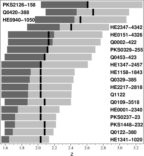
Figure 2: Limits of the Lyman-$\alpha$ forest along each line of sight in the survey. Different colors correspond to different redshift ranges. Light grey corresponds to the range between the Lyman-$\alpha$ and Lyman-$\beta$ emission lines where only Lyman-$\alpha$ absorption is expected. Dark grey corresponds to the range where Lyman-$\alpha$ is blended with other lines in the series. Black ticks correspond to the redshift at which Lyman$\beta$ is not redshifted enough to be observed.

3 Pixel optical depth method

In the highest SNR QSO spectrum obtained up to now, metals have been identified by direct detection of C iv absorption lines down to column densities as small as $N$(C iv) = 10^11.7 cm^-2 (Ellison et al. 2000). Most of these lines are associated with H i column densities larger than 10¹⁴ cm^-2 and are therefore believed to trace overdense regions such as filaments of the IGM web. Our data have usually a detection limit of about 10¹² cm^-2 in the C iv region outside the Lyman-$\alpha$ forest. To test for the presence of metals in gas of smaller H i optical depth, we use a variant of the pixel optical depth method (POD), that associates the H i optical depth with that in metals (mainly C iv and O vi) on a pixel by pixel basis (Cowie & Songaila 1998, Ellison et al. 2000, Aguirre et al. 2002).

The principle of the method is as follows. Once the Lyman-$\alpha$ forest is cleaned from all metals (see below), the H i Lyman-$\alpha$ optical depth is calculated in each pixel of the forest. When the Lyman-$\alpha$ line is saturated, other transition in the Lyman series are used. For each Lyman-$\alpha$ pixel, the observed optical depth in the metal transition at the same redshift is measured. Pixels in the Lyman-$\alpha$ forest are sorted according to their Lyman-$\alpha$ optical depth and are gathered in optical depth bins that contains a large number of pixels. Then the median of the associated metal optical depths is calculated in the predefined bins. The median is chosen instead of the mean to avoid a few pixels with high optical depth to bias the mean optical depth. In that way it is possible to test for the overall presence of metals in low density gas. The method has been extensively tested by Aguirre et al. (2002). Here we improve the method by carefully cleaning the Lyman-$\alpha$ forest for the presence of metals.

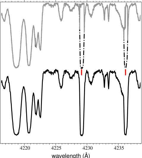
Figure 3: The Lyman-$\alpha$ forest (lower curve; here part of the HE 0151$-$4326 spectrum) is fitted consistently using the Lyman series. The automatic procedure is therefore able to detect the presence of metals. The upper curve shows the fit of the forest where the procedure has recognised the presence of the strong C iv system indicated by tick marks.

3.1 Determination of $\tau_{\rm HI}$ and cleaning the Lyman-$\alpha$ forest from metals

We want to estimate the Lyman-$\alpha$ optical depth in the largest number of pixels possible. For this we have to take into account that the absorption optical depth in any pixel can be due to several H i Lyman transitions at different redshift and also to possible metal lines associated with strong systems. If $z_{\rm em}$ is the emission redshift of the quasar, and 1215.67 and 1025.67 Å  are the wavelengths of the H i Lyman-$\alpha$ and Lyman-$\beta$ transitions, in the wavelength range [$\lambda_{\rm min}$,$\lambda_{\rm max}$] =  [(1+$z_{\rm em}$)$\times$1025.67,(1+$z_{\rm em}$)$\times$1215.67], only Lyman-$\alpha$ absorption is expected from H i. In the wavelength range $\lambda$ $<$ (1+$z_{\rm em}$)$\times$1025.67 the total absorption is due to the Lyman-$\alpha$ forest, the possible metal lines and also the absorptions in the different Lyman series transitions from the Lyman-$\alpha$ forest at higher redshift.

We start considering $\lambda^{\rm obs}_{\rm alpha}$ in the wavelength range [$\lambda_{\rm min}$,$\lambda_{\rm max}$] =  [(1+$z_{\rm em}$)$\times$1025.67,(1+$z_{\rm em}$)$\times$1215.67]. For each pixel, corresponding to $\lambda^{\rm obs}_{\rm alpha}$ = (1 + $z$)$\times$1215.67, we measure the effective optical depth in Lyman-$\alpha$ and calculate the corresponding effective optical depths at the positions, (1 + $z$)$\times$$\lambda^{\rm 0}_{\rm series}$, of all transitions in the Lyman series redshifted in the observed wavelength range,

$$\tau_{\rm series}=-{f_{\rm series}\over f_{\rm alpha}}ln[F({\lambda^{\rm obs}_{\rm alpha}\over 1215.67}\lambda^{\rm 0}_{\rm series})]$$ (1)

where $f_{\rm series}$ is the transition oscillator strength and $\lambda^{\rm 0}_{\rm series}$ the laboratory wavelength of the transition in the series. When the flux in a pixel is smaller than the noise rms at this position, we flag the pixel as a saturated pixel. The Lyman-$\alpha$ optical depth, $\tau_{\rm alpha}$ in the considered pixel at $\lambda^{\rm obs}_{\rm alpha}$, is taken to be the smallest of the above $\tau_{\rm series}$ that are larger than the noise rms at the corresponding position in the spectrum. This procedure allows us (i) to estimate the optical depth even if a transition is saturated; (ii) to avoid part of the blending effects. When all transitions are saturated, the pixel is flagged and is given a lower limit on $\tau$. Once $\tau_{\rm alpha}$ is estimated over the above wavelength range [$\lambda_{\rm min}$,$\lambda_{\rm max}$], it is possible to subtract to the spectrum the corresponding optical depths in all Lyman transitions. Then it is possible to go on with the determination of $\tau_{\rm alpha}$ over the wavelength range [$\lambda_{\rm min}$,$\lambda_{\rm max}$] =  [(1+$z_{\rm em}$)$\times$1025.67²/1215.67, (1+$z_{\rm em}$)$\times$1025.67] using the same procedure.

The advantage of this procedure is not only to increase the redshift range over which the study can be performed but to clean the Lyman-$\alpha$ forest from most of the polluting strong metal absorptions. Indeed, the strong metal absorptions are left over once the H i absorptions have been subtracted. Figure 3 illustrates how successful the procedure can be in recognising automatically strong absorptions due to metals in the forest on the basis of the forest properties only.

3.2 Cleaning the spectra

The spectra have been scrutinised to flag all portions of the lines of sight where strong metal lines hide the information we need. These regions and their complements (O vi and H i wavelength ranges in the forest, C iv wavelength range in the red) are removed from the analysis. This includes in particular strong Fe ii and Mg ii systems and all associated systems. The latter are characterised by partial covering factors and large $N$(C iv)/$N$(H i), $N$(N v)/$N$(H i) and $N$(O vi)/$N$(H i) column density ratios. When in doubt, we have kept the absorptions as in the system shown on figure  4. The latter is observed at $z_{\rm abs}=2.4178$ towards HE0151$-$4326, 42600 km.s^-1 from the emission redshift ($z_{\rm em}$ = 2.789).

This means that the C iv and O vi optical depths could be slightly overestimated although we are confident that enough care has been exercised and no obvious system has been missed. We have also restricted the analysis to absorptions located at least 3000 km s^-1 away from the emission redshift.

Figure 4: Portion of the spectrum of HE 0151$-$4326 centered at $z$=2.4178 showing a strong Lyman-$\alpha$ absorption line with no C iv absorption associated but two satellites H i absorptions have strong associated C iv and O vi absorptions. These satellites are narrow, there is no sign of strong displacement between H i, C iv and O vi, N v is absent and covering factor is unity: these lines are kept in the analysis and are not considered as ”associated” with the quasar.

3.3 Metal optical depth

Once the optical depth in the Lyman-$\alpha$ forest, $\tau_{\rm HI}$, is known, the corresponding optical depth of associated metal transitions at the same redshift can be derived.

To avoid the effects of blending, we use doublets such as C iv$\lambda\lambda$1548,1550 and O vi$\lambda\lambda$1031,1037 to secure the optical depth. For each of the doublets, the first line (#1 of rest wavelength $\lambda^{0}_{1}$) has an oscillator strength twice larger than the second line (#2 of rest wavelength $\lambda^{0}_{2}$). Therefore, the true optical depth in transition #1 must be twice larger than the true optical depth in transition #2. We therefore can impose that the two optical depths be consistent. Using the observed optical depths at the position of the two transitions, $\tau^{\rm obs}_{1}$ and $\tau^{\rm obs}_{2}$, we want to determine the best estimator of the optical depth, $\tau_{1}$, in the first transition. Starting from the smallest wavelength, we calculate for each pixel of wavelength $\lambda_{1}$, the observed optical depth at this position $\tau^{\rm obs}_{1}$ = $-$ln($F_{1}$) and the observed optical depth $\tau^{\rm obs}_{2}$ = $-$ln($F_{2}$) at a position $\lambda_{2}$ = $\lambda_{1}\times\lambda^{0}_{2}$/$\lambda^{0}_{1}$.

Two cases require special consideration. The potential absorption is said to be ”In the noise” if $F>1-\kappa\times\sigma$ with $\sigma$ the rms of the noise in the corresponding pixel and $\kappa$ = 3. When $F<\kappa\times\sigma$, the absorption is said to be ”Saturated”.

We use for $\tau_{1}$, either $\tau^{\rm obs}_{1}$ or $\tau^{\rm obs}_{2}\times f_{1}/f_{2}$ depending on the status of the absorptions. The different cases are summarised in Table 2. In the case the two lines are neither in the noise nor saturated (the lines are ”OK”), or if #1 is ”OK” and #2 is ”In the noise” (cases denoted ”Check” in the Table), some additional test has to be performed. First $F_{1}$ is used to predict $F^{\rm exp}_{2}$ that is the expected flux $F_{2}$ in case the absorptions are only due to unblended lines from the doublet considered. If $F^{\rm exp}_{2}\geq(F_{2}-\sigma_{2})$, then $\tau_{1}$ = $\tau^{\rm obs}_{1}$. If not, $\tau_{1}$ = $\tau^{\rm obs}_{2}\times f_{1}/f_{2}$. Once $\tau_{1}$ is defined and if $F_{\rm 1}$ $<$ $1-\kappa\times\sigma_{1}$, we replace $\tau_{2}^{\rm obs}$ at position $\lambda_{2}$, by $\tau_{2}^{\rm obs}-\tau_{1}\times f_{2}/f_{1}$. This corresponds to a self-contamination correction.

Table 2: Determination of $\tau_{1}=\tau_{\rm metal}$

		Line 1
		Saturated	In the noise	OK
	Saturated	Lower limit	$\tau_{1}^{\rm obs}$	$\tau_{1}^{\rm obs}$
Line 2	In the Noise	$\tau_{2}^{\rm obs}\times f_{1}/f_{2}$	$\tau_{1}^{\rm obs}$	Check
	OK	$\tau_{2}^{\rm obs}\times f_{1}/f_{2}$	$\tau_{1}^{\rm obs}$	Check

3.4 Simulations

To check our two procedures, normalisation of the spectrum and recovery of the C iv optical depth, we simulated QSO spectra drawing H i absorption lines at random from a population with the same column density and Doppler parameter distributions as observed, using the same spectral resolution as in the UVES data and adding noise. We use S/N = 10000 to simulate perfect data and S/N = 70 to simulate observations. We include C iv absorption at the same redshift as H i, assuming a fixed log $\tau$(C iv)/$\tau$(H i) ratio. We recover $\tau$(C iv) versus $\tau$(H i) and plot results in Fig. 5 for log $\tau$(C iv)/$\tau$(H i) = $-$2.5 (squares), $-$3 (crosses), $-$3.5 (circles) and $-$10 (diamond) to simulate data without any enrichment. We applied the same pixel-to-pixel procedure after normalisation of the data either with the known continuum (top panels) or using our normalisation procedure (bottom panels). We plot $\tau$(C iv) recovered by the procedure versus $\tau$(H i). It can be seen that we can recover correctly $\tau$(C iv) in all cases down to log $\tau_{\rm HI}$ $\sim$ 0. The presence of metals is revealed by a correlation between $\tau_{\rm HI}$ and $\tau_{\rm metals}$ and the plateau at small H i optical depths is a consequence of limited S/N ratio. It is clear that these simulations give us full confidence in our results.

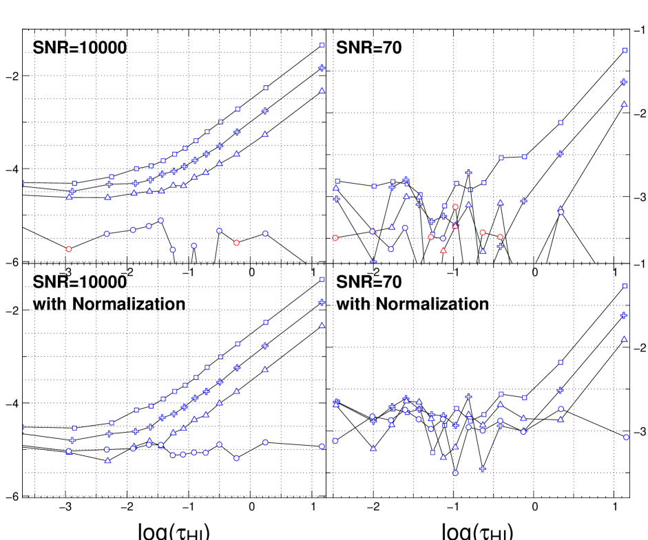
Figure 5: Test of the normalisation and pixel-by-pixel procedures. We simulate QSO spectra drawing H i absorption lines at random from a population with the same column density and Doppler parameter distributions as observed, using the same spectral resolution as the UVES data and adding noise, S/N = 10000 in the left panels and S/N = 70 in the right panels. We include C iv absorption at the same redshift as H i assuming some fixed ratio, log $\tau$(C iv)/$\tau$(H i) = $-$2.5 (squares), $-$3 (crosses), $-$3.5 (triangles) and $-$10 (diamonds). We apply the same pixel-to-pixel procedure (all panels) to the data without normalisation (the continuum is assumed to be known; upper panels) and with normalisation (using our automatic procedure) of the spectra (bottom panels). We plot $\tau$(C iv) recovered by the procedure versus $\tau$(H i). It can be seen that we can recover correctly $\tau$(C iv) in all cases down to log $\tau$ $\sim$ 0.

4 Results

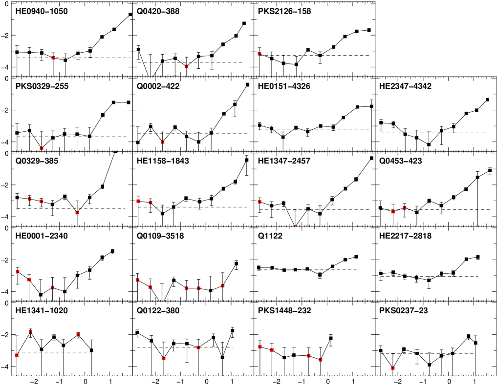
Figure 6: C iv optical depth versus H i optical depth for individual quasars in the sample.

Figure 7: O vi optical depth versus H i optical depth for the 19 individual quasars in the sample.

We apply the following procedure either for one line of sight or for the complete data set, combining all lines of sight. Pixels in the Lyman-$\alpha$ forest are sorted in order of increasing H i Lyman-$\alpha$ optical depth and are gathered in predefined bins. In each of the bins, the median of the corresponding $\tau_{\rm metal}$, measured at the same redshift, is then calculated. Using the median instead of the mean avoids the measurement to be biased by the presence of a few strong absorptions. Individual plots for the nineteen lines of sight are shown for C iv and O vi in Fig. 6 and 7, respectively.

4.1 Presence of C iv

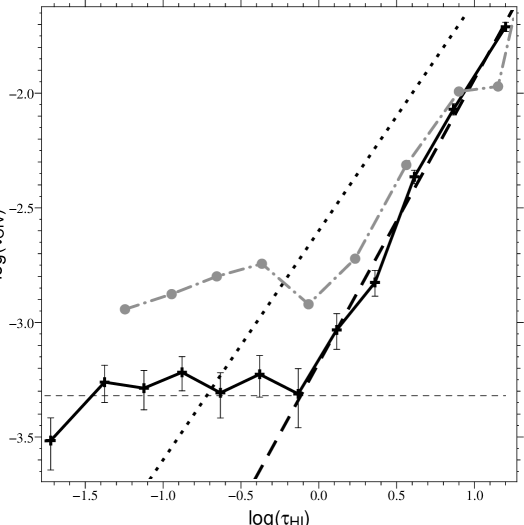
Figure 8: Median of C iv optical depth versus median of H i optical depth is plotted with black cross. Only pixels with velocity difference larger than 3000 km s^-1 compared to the emission redshift of the quasar are used. Grey circles correspond to the previous finding by Ellison et al. (2000). The dotted line is drawn for illustration and corresponds to log C iv/H i $\sim$ $-$2.6 . The dashed thick line is a fit to the data for $\log\tau_{\rm HI}>0$; $\log\,\tau_{\rm CIV}\,=\,1.3\times\log\,\tau_{\rm HI}-3.2$. The horizontal dashed line corresponds to the median of $\tau_{\rm CIV}$ for log $\tau_{\rm HI}$ $<$ $-$1.3.

We plot in Fig. 8 the median of the C iv optical depth versus the median of the H i optical depth when combining the whole sample. It can be seen that there is an excess of C iv for $\tau_{\rm HI}$ $>$ 1. This excess is present for nearly all the individual lines of sight (see Fig. 6). For $\tau_{\rm HI}$ $<$ 1, there is no detection of C iv. In particular, the apparent optical depth is statistically the same and consistent with zero for all the bins corresponding to log $\tau_{\rm HI}$ $<$ 0.

The thick dashed line corresponds to a fit to the data for log $\tau_{\rm HI}$ $>$ 0: log $\tau_{\rm CIV}$ = 1.3$\times$log $\tau_{\rm HI}$ $-$ 3.2. The dotted diagonale line is drawn for illustration and corresponds to log($\tau_{\rm CIV}/\tau_{\rm HI}$) = $-$2.6. It can be seen that the diagonale line is rejected by our data. Indeed, the present data are inconsistent with a uniform distribution of C iv in the Lyman-$\alpha$ forest with constant $\tau_{\rm CIV}/\tau_{\rm HI}$ ratio. On the contrary our results strongly suggest that the C iv/H i ratio increases with increasing $\tau_{\rm HI}$. It is also apparent that for log $\tau_{\rm HI}$ $\sim$ 0, log(C iv/H i) $<$ $-$3.2. Although the results by Schaye et al. (2003) favor a slope closer to the diagonale than what we observe, their error bars are larger and their measurements are consistent with our findings.

It is important to note also that the scatter in the C iv optical depth is very similar at different H i optical depths. This means that although the mean C iv optical depth decreases with decreasing $\tau_{\rm HI}$, large C iv optical depths can be seen at nearly any H i optical depth. This is illustrated in Fig. 4 where a strong Lyman-$\alpha$ system is seen with no C iv absorption associated down to our detection limit $\sim$10¹² cm^-2, but two satellite H i absorptions have strong associated C iv and O vi absorption (see also Bergeron et al. 2002). It must be noted that these systems have quiet dynamics (the different absorptions of C iv, O vi and H i are fairly well centered on top of each others), they do not show evidence for partial covering factors and have very little or no N v associated absorption. Therefore, their properties strongly differ from those of systems associated with the quasar and they must be truly intervening systems.

4.2 Presence of OVI

Figure 9: The median O vi optical depth is plotted versus the median H i optical depth. The crosses are the observed data, other curves are simulations where the ratio log O vi/H i is given fixed values, $-$5.0 (no metals), $-$2.5, $-$2.0, $-$1.7, $-$1.5 from the curve labelled (a) to the one labelled (e), respectively

Schaye et al. (2000) performed a similar pixel-by-pixel search for O VI absorption in eight high-quality quasar spectra spanning the redshift range $z$ = 2.0–4.5. In the redshift range 2 $<$ $z$ $<$ 3, they stated to detect O vi in the form of a positive correlation between the H i Lyman-$\alpha$ optical depth and the optical depth in the corresponding O vi pixel, down to $\tau_{\rm HI}$ $\sim$ 10^-1. On the contrary, they did not detect O vi at $z>$ 3 and considered this is consistent with the enhanced photoionization from a hardening of the UV background below $z<3$, although this could also be caused by the high level of contamination from Lyman series lines.

Figure 10: Median O vi optical depth versus median H i for pixels located at less than 500 km s^-1 (upper dashed curve) or less than 300 km s^-1 (upper dotted curve) from strong absorptions ($\tau_{\rm HI}\leavevmode\nobreak\ >\leavevmode\nobreak\ 4$) and for pixels located at more than 500 km s^-1 (lower dashed curve) or more than 300 km s^-1 (lower dotted curve) from strong absorptions.

It can be seen from Fig. 9 that our data confirm the detection of O vi down to $\tau_{\rm HI}$ $\sim$ 0.2 that is at smaller H i optical depth than for C iv which is seen down to $\tau_{\rm HI}$ $\sim$ 1 only. To investigate if the signal for 0.2 $<$ $\tau_{\rm HI}$ $<$ 1 comes from all parts of the spectrum however, we have divided the sample into two subsamples. The first subsample contains all H i pixels located within $\Delta v$ from a strong absorption with $\tau_{\rm HI}$ $>$ 4 and the second subsample contains all other pixels. We then vary $\Delta v$. It can be seen on Fig. 10 that for $\Delta v$ $\leq$ 300 km s^-1, the signal significantly increases for the first subsample. This means that O vi is predominantly seen in the vicinity of strong Lyman-$\alpha$ absorption lines. Indeed, the signal disappears for the second subsample; there is no O vi absorption for 0.2 $<$ $\tau_{\rm HI}$ $<$ 1. This new result strongly suggests that the O vi absorption arises mostly in regions close in space to those responsible for strong H i absorptions and a most likely explanation is that the O vi phase is part of winds flowing away from overdense regions.

To derive a quantitative limit on the amount of O vi present in the IGM, we have performed simulations of the metal enrichment of the Lyman-$\alpha$ forest. Artificial spectra are created drawing absorption lines at random from a population with column density and Doppler parameter distributions consistent with those observed (Petitjean et al. 1993, Hu et al. 1995, Kirkman and Tytler 1997, Kim et al. 2000). The number of lines is adjusted so that the mean absorption of the simulated spectra is the same as the observed one. Although this is probably a rough assumption, constant O vi/H i ratio is assumed and O vi absorption is added accordingly. Noise consistent with the data is added and the whole procedure described in Section 3 is applied to the simulated spectra. Results are plotted in Fig. 9. It can be seen that data are consistent with log O vi/H i $\sim$ $-$2, a value within the range found for individual O vi systems (Bergeron et al. 2002).

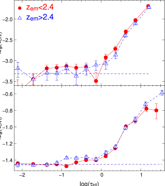
Figure 11: The C iv (top panel) and O vi (bottom panel) optical depth is plotted versus the H i optical depth for $z$ $<$ 2.4 (filled circles and solid line) and $z$ $>$ 2.4 (triangles and dashed line).

4.3 Evolution with redshift

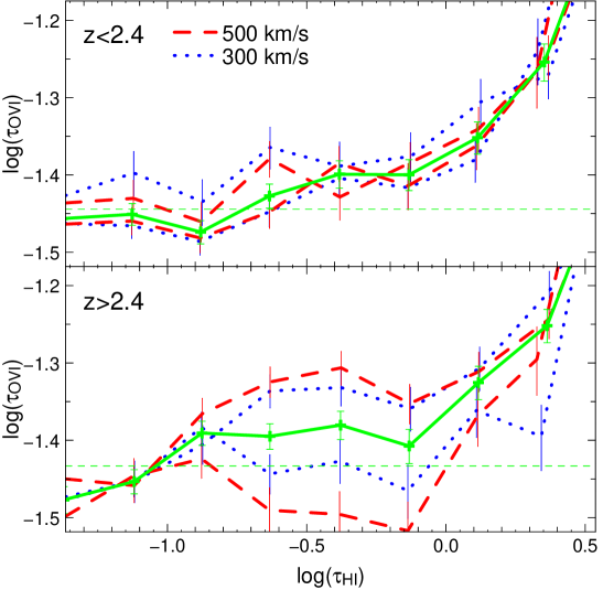
Figure 12: Same as figure 10 for the two redshift bins, $z$ $<$ and $>$ 2.4.

We have divided the sample in two redshift bins with similar number of pixels in each bin, $z$ $>$ and $<$ 2.4. We plot in Fig. 11 C iv (top panel) and O vi (bottom panel) optical depths versus H i optical depth for $z$ $<$ 2.4 (filled circles and solid line) and $z$ $>$ 2.4 (triangles and dashed line). It can be seen that C iv optical depth shows mild cosmic evolution when no evolution is detected in $\tau_{\rm OVI}$. The most interesting feature however is that the excess of O vi optical depth at log $\tau_{\rm HI}$ $\sim$ $-$0.5 is more important in the high redshift bin. Note that this signal is due to the three lines of sight toward quasars with the highest emission redshifts. Moreover, if we apply the same procedure as previously, we find that, at $z$ $<$ 2.4, the O vi absorption does not seem to be related to strong lines when the relation is apparent at larger redshift (see Fig 12). As this signal is probably related to galactic winds, this may be an indication that galactic winds are more prominent at higher redshift.

5 Conclusion

We have used a pixel-by-pixel analysis to investigate the presence of metals in the inter galactic medium. We have measured the median optical depth of C iv$\lambda$1548 and O vi$\lambda$1031 absorptions versus the H i Lyman-$\alpha$ optical depth of the gas at a mean redshift $z$ = 2.6 using 19 lines of sight observed at high spectral resolution ($R$ = 45000) and high and homogeneous S/N ratio (approximately 35 and 70 per pixel over, respectively, the O vi and C iv wavelength ranges). Great care has been exercized to determine the continuum.

We have carefully determined the H i optical depth by taking into account the information in the Lyman series (usually Lyman-$\beta$ and Lyman-$\gamma$). We have also carefully removed from the spectra all wavelength ranges that are polluted by strong intervening absorptions from metal line systems, in particular Mg ii and Fe ii systems, and from associated systems.

We find that the gas is enriched in carbon and oxygen for $\tau_{\rm HI}$ $>$ 1. Contrary to previous claims, there is no indication that C iv absorption is statistically associated with gas of H i Lyman-$\alpha$ optical depth smaller than 1. In addition, our observations strongly suggest that the C iv/H i ratio decreases with decreasing $\tau_{\rm HI}$. We observe that for $\tau_{\rm HI}$ $\sim$ 1, log $\tau_{\rm CIV}$/$\tau_{\rm HI}$ $<$ $-$3.2 which corresponds to log C iv/H i$<$ $-$3.3 assuming $b_{\rm HI}/b_{\rm CIV}=2$ and a Voigt profile or log C iv/H i$<$ $-$3.0 assuming $b_{\rm HI}=b_{\rm CIV}$. This does not prevent a small fraction of the low $\tau_{\rm HI}$ gas from being associated with strong metal lines (see Fig. 4) indicating that enrichment is highly inhomogeneous.

We detect the presence of O vi for $\tau_{\rm HI}$ $>$ 0.2, consitent with a constant ratio log $\tau_{\rm OVI}$/$\tau_{\rm HI}$ $\sim$ $-$2.0 corresponding to log O vi/H i $\sim$ $-1.75$ assuming $b_{\rm HI}/b_{\rm OVI}=2$ and a Voigt profile or log O vi/H i $\sim$ $-1.45$ assuming $b_{\rm HI}=b_{\rm OVI}$ . We show that for 0.2 $<$ $\tau_{\rm HI}$ $<$ 1, the O vi absorption is associated with gas located within $\sim$300 km s^-1 from strong H i lines. This suggests that the O vi phase is probably part of winds flowing away from overdense regions.

It is therefore not possible to conclude that metals are present in the most teneous regions of the IGM ($\tau_{\rm HI}$ $<$ 1 corresponding to overdensities of about 1 to 3 at $z$ $\sim$3 and 2 respectively) far away from overdense regions.

- (1) Aguirre, A., Schaye, J., & Theuns, T. 2002, ApJ, 576, 1
- (2) Bergeron, J., Aracil, B., Petitjean, P., & Pichon, C. 2002, A&A, 396, L11
- (3) Bi, H., & Davidsen, A. F. 1997, ApJ, 479, 523
- (4) Carswell, R. F., Schaye, J., & Kim, T. S. 2002, ApJ, 578, 43
- (5) Cen, R., Miralda-Escudé, J., Ostriker, J. P., & Rauch, M. 1994, ApJ, 437, L9
- (6) Cowie, L. L., Songaila, A. 1998, Nature, 394, 44
- (7) D’Odorico, S., Cristiani, S., Dekker, H., Hill, V., Kaufer, A., Kim, T., & Primas, F. 2000, Proc. SPIE, Vol. 4005, p. 121
- (8) Ellison, S. L., Songaila, A., & Pettini, M. 2000, AJ, 120, 1175
- (9) Ferrara, A., Pettini, M., & Shchekinov, Y. 2000, MNRAS, 319, 539
- (10) Hernquist, L, Katz, N., Weinberg, D. H., & Miralda-Escudé, J. 1996, ApJ, 457, L51
- (11) Hu, E. M., Kim, T., Cowie, L. L., Songaila, A., &Rauch, M. 1995, AJ, 110, 1526
- (12) Kim, T.-S., Carswell, R. F., Cristiani, S., D’Odorico, S., & Giallongo, E. 2002, MNRAS, 335, 555
- (13) Kirkman, D., & Tytler, D. 1997, ApJ, 484, 672
- (14) Lu, L., Sargent, W. L. W., Barlow, T. A., & Rauch, M. 1998, astro-ph/9802189
- (15) Petitjean, P. 2001, ApSSS 277, 517
- (16) Petitjean, P., Mücket, J., Kates, R. E. 1995, A&A, 295, L9
- (17) Petitjean, P., Webb, J. K., Rauch, M., Carswell, R. F., & Lanzetta, K. 1993, MNRAS, 262, 499
- (18) Schaye, J., Aguirre, A., Kim, T. S., Theuns, T., Rauch, M., & Sargent, W. L. W. 2003, astro-ph/0306469
- (19) Schaye, J., Rauch, M., Sargent, W. L. W., & Kim, T. S. 2000, ApJ, 541, L1
- (20) Simcoe, R.A., Sargent, W. L. W., Rauch, M. 2002, ApJ, 578, 737
- (21) Songaila, A. 1998, AJ, 115, 2184
- (22) Tytler, D., Fan, X. M., Burles, et al., 1995, QSO Absorption Lines, Proceedings of the ESO Workshop Held at Garching, Germany, 21 - 24 November 1994, edited by Georges Meylan. Springer-Verlag Berlin Heidelberg New York. Also ESO Astrophysics Symposia, p. 289