Dual Cometary H II  Regions in DR21: Bow Shocks or Champagne Flows?

Abstract

The DR 21 massive star forming region contains two cometary H II  regions, aligned nearly perpendicular to each other on the sky. This offers a unique opportunity to discriminate among models of cometary H II  regions. We present hydrogen recombination and ammonia line observations of DR 21 made with the Very Large Array. The velocity of the molecular gas, measured from NH₃ emission and absorption lines, is constant to within $\pm 1$  km s^-1 across the region. However, the radial velocity of the ionized material, measured from hydrogen recombination lines, differs by $\approx 9$  km s^-1 between the “heads” of the two cometary H II  regions and by up to $\approx 7$  km s^-1  from that of the molecular gas. These findings indicate a supersonic velocity difference between the compact heads of the cometary regions and between each head and the ambient molecular material. This suggests that the observed cometary morphologies are created largely by the motion of wind-blowing, ionizing stars through the molecular cloud, as in a bow shock model.

1 Introduction

Compact H II  regions are commonly observed in massive star forming regions (Mezger, Schraml, & Terzian, 1967; Garay & Lizano, 1999). Reid & Ho (1985) first noted that a compact H II  region in the G34.3$+$0.2 star forming region had a cometary appearance, with a bright head and a diffuse tail. Rather than being a unique or even a rare source, G34.3$+$0.2 became the archetypal example of a class of sources now called cometary H II regions. The survey of Wood & Churchwell (1989) revealed that 20% or more of compact H II  regions have cometary morphology.

Several models explaining the cometary appearance of compact H II regions have been proposed and actively debated. Reid & Ho (1985) first suggested that the cometary appearance of G34.3$+$0.2 could result from relative motion between an ionizing star and its surrounding molecular material, analogous to elongated structures predicted for such stars moving rapidly though the more diffuse interstellar medium (Weaver et al., 1977). This led to the “bow shock” model, which postulates supersonic motion of a star, with a strong stellar wind, through a molecular cloud (van Buren, Mac Low, Wood, & Churchwell, 1990). An alternative model for the formation of cometary H II regions is the “Champagne flow” model. This model assumes that the ionizing star is nearly stationary with respect to the molecular cloud, but that the material surrounding the star has a steep density gradient (Israel, 1978; Tenorio-Tagle, 1979). Since the size and shape of an H II  region are determined by the balance of ionization and recombination rates, an H II  region will be “extended” in the direction of lowest density. In a uniform density gradient, this results in a parabolic shape for the ionized region, which can appear cometary. Other models for cometary H II regions are discussed by Gaume, Fey, & Claussen (1994); Raga (1986); Gaume & Mutel (1987).

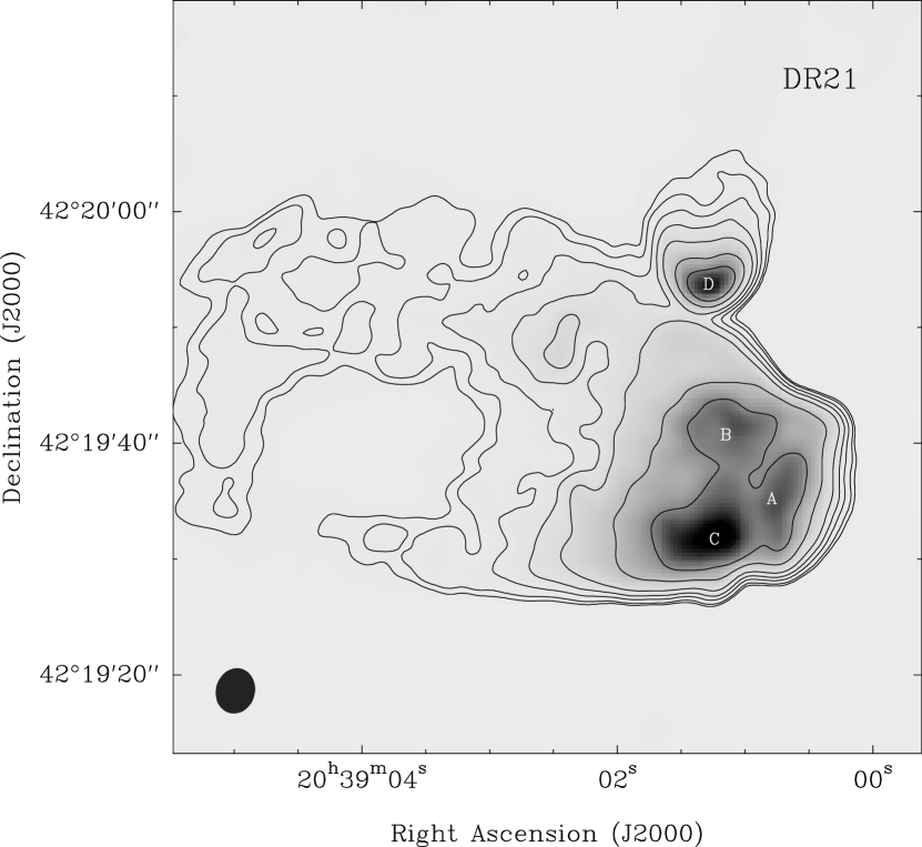
Figure 1: Continuum emission from the dual cometary H II regions in DR 21 at 6-cm wavelength. Contour levels are 0.01, 0.02, 0.05, 0.1, 0.2, 0.5, 1, and 2 Jy beam^-1. The $\approx 1\hbox to0.0pt{.\hss}{{}^{\prime\prime}}7$ FHWM beam is indicated by the filled ellipse near the lower left corner. Ionized condensations labeled A, B, C, & D by Harris (1973) are indicated.

Harris (1973) published a high resolution map at 5 GHz of the massive star forming region DR 21. She noted two H II regions: a compact northern (D) and an extended southern source, with the southern source resolved into “three very compact condensations” (A, B, & C). Most discussion in the literature of these H II regions has followed the nomenclature of Harris, as well as her interpretation of the southern H II region’s condensations as being independent compact sources excited by different stars. We recently mapped this region with higher angular resolution and sensitivity than Harris and discovered that the northern and southern H II regions are both cometary H II regions with nearly perpendicular symmetry axes projected on the sky. Fig. 1 shows the 6-cm wavelength continuum emission from these sources, obtained from VLA B-configuration data taken on 2001 April 23.

Finding twin cometary H II regions in one star forming region provides a possibly unique opportunity to investigate the relative motion of cometary H II regions, as well as their internal velocity structures and overall motion with respect to nearby molecular material. Since the bow shock and Champagne flow models predict different velocity structures, we undertook high angular resolution, spectral-line observations in order to distinguish between these models. We used the Very Large Array (VLA) of the National Radio Astronomy Observatory (NRAO) to map two high-frequency radio recombination lines, in order to study motions in the plasma, and two ammonia (NH₃) transitions, in order to study motions in the surrounding molecular material.

2 Observations and Data Analysis

We observed DR 21 in two hydrogen recombination lines and two NH₃ transitions using the VLA on 2001 December 23. The array was in the D-configuration, with a minimum baseline of 0.033 km and a maximum baseline of 1.03 km. We obtained approximately 1 hour of on-source integration time each for the H53$\alpha$ line (42951.97 MHz rest frequency) and the H66$\alpha$ line (22364.17 MHz rest frequency). The bandwidth for both recombination line observations was 12.5 MHz, which was divided into 32 channels of 390.625 kHz (or 2.73 and 5.25  km s^-1 for H53$\alpha$ and H66$\alpha$, respectively). The NH₃  (1,1) and (2,2) transitions were observed in both right and left circular polarization with bandwidths of 3.125 MHz, divided into 64 channels of 48.828 kHz (or 0.62  km s^-1), and we obtained a total on-source integration time of $\approx 2$ hours.

For both the recombination and NH₃  line observations, the band center was set to an LSR velocity of $-2.0$  km s^-1 . The source 1331+305 was observed as a primary flux calibrator, 2015+371 as a secondary calibrator, and 2253+161 as a bandpass calibrator. We used the NRAO Astronomical Image Processing System (AIPS) to edit, calibrate, image and display the data. Initial calibration and subsequent self-calibration were done using the “channel 0” data set (encompassing the central 75% of the original bandwidth).

A preliminary flux scale for the H53$\alpha$ observations at 43 GHz was based on a flux density of 1.47 Jy for 1331+305. This flux density is quite uncertain. Therefore, after standard calibration, we measured the continuum flux density of the brightest portion of the southern cometary H II region at 22 and 43 GHz and adjusted the 43 GHz fluxes to give the expected optically thin spectral index of $-0.1$ for an H II region. This required multiplying the H53$\alpha$ data by a factor of 1.24.

Line-minus-continuum (u,v)-databases were created by fitting a straight line to the (continuum) signal in spectral channels with little or no line emission or absorption and then subtracting this fit from the entire spectrum. Because the recombination lines are very broad, we could only use a few channels on each side of the H66$\alpha$ line to measure the continuum. We used the same observing bandwidth for the H53$\alpha$ observations and were able to use only a few channels near the low-frequency end of the spectrum as off-line channels. Thus, we removed only a constant continuum level for the H53$\alpha$ data. (However, as discussed below, for both recombination lines we ultimately removed any residual continuum emission by fitting a sloped baseline to spectra generated from the line-minus-continuum maps.) A pure continuum (u,v)-database was also constructed from the off-line channel baseline fits, evaluated at the center frequency of the original bands. A 22 GHz continuum map made from the baseline fits for the H66$\alpha$ data is shown in Fig. 2.

Figure 2: Continuum emission from the dual cometary H II regions in DR 21 at 1.3-cm wavelength. Contour levels are 0.02, 0.05, 0.1, 0.2, 0.5, 1, and 2 Jy. Dotted boxes indicate “long-slit” areas over which spectra were summed for Gaussian fitting of the hydrogen recombination lines. Dashed boxes indicate the areas where NH₃ emission spectra were generated; areas for NH₃ absorption spectra cover most of the northern and southern H II regions and correspond approximately to regions N/1 to N/3 and S/1 to S/3, respectively. Labels near the boxes indicate position listed in Table 1. Line-center velocities from Gaussian fitting are given in  km s^-1 with respect to the LSR in bold face in the center of the boxes. For the hydrogen recombination velocities, the average of H66$\alpha$ and H53$\alpha$ fits are indicated, where both lines were detected.

The calibrated line-minus-continuum data were used to generate image cubes. For the hydrogen recombination line data, we made image cubes with tapered (6^′′ beam) and un-tapered (3^′′ beam) (u,v)-data, and used the tapered cubes to analyze the large southern H II region and the un-tapered cubes for the smaller northern H II region. Next, we generated spectra by summing the emission over “long-slits,” approximately perpendicular to the major axes of the two cometary H II regions. We chose such long-slits in order to increase signal-to-noise ratios and to facilitate comparison to models which generally have axial symmetry about the cometary axis. The positions of these long-slits are indicated on Figure 2 and the resulting spectra for the H66$\alpha$ transition are shown in Figure 3. In order to determine Doppler velocities, we fitted a Gaussian line profile to these spectra. The amplitude, central velocity, and FWHM of the Gaussian line profile were adjustable parameters, as well as two parameters allowing for a linear spectral baseline. For both recombination lines, the spectral baselines typically sloped by about $\pm 10$% of the peak amplitude of the line. Results of the Gaussian fits are given in Table 1 and Figure 3. While formal fitting errors usually were $<0.3$  km s^-1, we estimate a more realistic error that allows for modeling uncertainty of $\approx 1$  km s^-1.

We analyzed both NH₃  transitions and obtained nearly identical kinematic information from the two transitions, and for brevity we report here only the NH₃ (1,1) transition results. The NH₃ (1,1) transition main-hyperfine component at a rest frequency of 23694.496 MHz was used to obtain Doppler velocities. Offset from the continuum sources, we detected the NH₃ in emission and produced spectra summed over long-slits (see Fig. 2), as for the hydrogen recombination lines. Toward the cometary H II regions, we detected NH₃ in absorption and spectra were obtained by summing over regions that enclosed most of the continuum emission from each region. The spectra showed a small, but distinct, baseline curvature. Thus, we fitted a second-order baseline in addition to Gaussian lines to the spectra. The Gaussian fits to the main-lines are given in Table 1. In Figure 3 we show the observed spectra and the best-fitting (three) Gaussians for the NH₃ main- and inner satellite-hyperfine components toward the H II regions and the H66$\alpha$ lines at positions along the cometary axes of the southern and northern H II regions.

Figure 3: NH₃ and H66$\alpha$  spectra toward the southern (left panels) and northern (right panels) cometary H II regions in DR 21. Dotted vertical lines give the velocity for the molecular material as indicated by the NH₃  main-hyperfine line absorption. Dashed sloping lines indicate the velocity of the ionized material, from the average of the H66$\alpha$ and H53$\alpha$ line fits, as one observes from head toward tail (from top to bottom plots) along the cometary axes of the H II regions.

Table 1: Gaussian Fit Parameters¹

HII Region/	S	vLSR	FWHM
Position	(Jy)	( km s-1)	( km s-1   )
H$66\alpha$
S/1	$0.398\pm 0.009$	$-2.6\pm 0.3$	$30.9\pm 1.0$
S/2	$1.132\pm 0.013$	$-2.5\pm 0.2$	$30.9\pm 0.5$
S/3	$0.770\pm 0.011$	$-0.8\pm 0.2$	$31.3\pm 0.7$
S/4	$0.168\pm 0.005$	$+0.2\pm 0.5$	$35.4\pm 1.6$
N/1	$0.145\pm 0.002$	$+5.9\pm 0.2$	$23.9\pm 0.4$
N/2	$0.186\pm 0.002$	$+5.1\pm 0.2$	$26.7\pm 0.5$
N/3	$0.038\pm 0.001$	$+4.1\pm 0.6$	$29.3\pm 1.6$
N/4	$0.009\pm 0.001$	$-0.5\pm 1.6$	$29.3\pm 4.5$
H$53\alpha$
S/1	$0.686\pm 0.027$	$-3.9\pm 0.4$	$33.4\pm 1.6$
S/2	$2.075\pm 0.029$	$-3.6\pm 0.2$	$31.9\pm 0.6$
S/3	$1.266\pm 0.016$	$-2.2\pm 0.2$	$31.5\pm 0.6$
N/1	$0.219\pm 0.004$	$+5.8\pm 0.2$	$23.2\pm 0.5$
N/2	$0.301\pm 0.006$	$+5.5\pm 0.2$	$26.3\pm 0.7$
NH3 (1,1)
A	$+0.116\pm 0.004$	$-1.6\pm 0.1$	$1.3\pm 0.1$
B	$+0.188\pm 0.008$	$-1.4\pm 0.1$	$1.3\pm 0.1$
Southern	$-1.157\pm 0.038$	$-1.6\pm 0.1$	$2.4\pm 0.1$
Northern	$-0.022\pm 0.002$	$-1.4\pm 0.2$	$4.5\pm 0.6$
C	$+0.079\pm 0.005$	$-2.7\pm 0.1$	$1.4\pm 0.1$
D	$+0.023\pm 0.004$	$-2.6\pm 0.2$	$2.7\pm 0.6$

3 Discussion

The first explanation proposed for the cometary H II  region morphology (Reid & Ho, 1985) invoked relative motion between an ionizing star and its external molecular environment. For the archetypal cometary H II region, G34.3$+$0.2, Reid & Ho (1985) noted the presence of a supernova remnant to the west of the cometary region’s “head” and suggested that a stellar wind from the supernova’s precursor star might be responsible for the H II  region’s cometary shape. The bow shock model, developed to explain cometary H II regions (van Buren, Mac Low, Wood, & Churchwell, 1990; Mac Low, van Buren, Wood, & Churchwell, 1991; van Buren & Mac Low, 1992), expanded upon this suggestion. It requires highly supersonic motion of a wind-blowing, ionizing star through dense surrounding material. On the other hand, a cometary appearance can also result from the ionization/recombination balance in a region with a strong density gradient, often called a Champagne flow (Israel, 1978; Tenorio-Tagle, 1979). In addition, other forces may play a role in shaping cometary H II regions (Gaume, Fey, & Claussen, 1994).

In this section, we first address the possibility that, in regions where ionized gas flows rapidly, hydrogen recombination line velocities may be difficult to interpret. Next, we briefly outline the dominant kinematic features of the bow shock and Champagne flow models. Finally, we compare the observed velocities of the ionized and molecular material to these models and argue that they are mostly consistent with the predictions of the bow shock model.

3.1 Are Recombination Lines Reliable Velocity Indicators?

We observed two hydrogen recombination lines in order to assess if the velocities measured by these lines differ significantly. Berulis & Ershov (1983) and Keto, Welch, Reid, & Ho (1995) discussed such an effect for W3OH, with line-center velocities shifting by $\approx 22$  km s^-1 between the H110$\alpha$ and H35$\alpha$ lines. The shift in observed line-center velocity with transition is large for high principal quantum number (low frequency) transitions and asymptotically approaches a constant at low principal quantum number (high frequency) transitions. Keto et al. suggest that this transition-dependent velocity shift results from a combination of a large velocity gradient in the ionized material and a strong increase in line-width for higher principal quantum number transitions, owing to collisional broadening. Since, for electron densities $\mathrel{\hbox{\raise 2.15277pt\hbox{$<$}\hbox to0.0pt{\hss\lower 2.15277pt\hbox{$\sim$}}}}10^{7}$ cm^-3, collisional broadening is small for the H66$\alpha$ and lower principal quantum number transitions, we would expect that our recombination lines would not be sensitive to this complication.

For DR 21, we observe almost no shift in velocity between the H66$\alpha$ and H53$\alpha$ lines. The velocities of the H66$\alpha$ and H53$\alpha$ lines agree within 2  km s^-1  at all locations. For the northern H II region, the agreement is within the joint uncertainties ($<0.3$  km s^-1). For the southern H II region, the H53$\alpha$  lines appear blue shifted by about $1.3$  km s^-1  compared to the H66$\alpha$ lines at the same positions on the sky. The spectral baselines in the two transitions tended to slope in opposite directions, and small correlations between the spectral slopes and the center velocities might contribute to these small shifts.

Roelfsema, Goss, & Geballe (1989) mapped H76$\alpha$ recombination lines toward several positions over the DR21 H II regions. The dual-cometary structure, clearly visible in our Fig. 1 at 6 cm wavelength, is not as evident in their 14.7 GHz continuum image, and they did not use long-slits to measure velocities along the symmetry axes of the cometary H II regions. Instead they formed spectra at local peaks in the radio brightness, including one in the northern and five in the southern H II region. Toward the northern H II region (their position D) the H76$\alpha$ line peaked at $4.6$  km s^-1, in good agreement with the average of our regions N/1 through N/3 which span velocities of 4.1 to 5.9  km s^-1. Toward the head of the southern H II region, Roelfsema, Goss, & Geballe (1989) measured a velocity (at their position A) of $-4.1$  km s^-1 which compares well with our measurement of $-3.3$  km s^-1 for region S/1. Also, their H76$\alpha$ measurements at positions B and C yielded velocities of $-1.2$ and $-3.2$  km s^-1; these positions if combined correspond to summing our regions S/2 and S/3 for which we measure velocities of $-1.6$ and $-3.0$  km s^-1. Again this indicates good agreement between the H76$\alpha$ measurements of Roelfsema, Goss, & Geballe (1989) and ours at H66$\alpha$ and H53$\alpha$.

In conclusion, since (1) on average the H76$\alpha$, H66$\alpha$, and H53$\alpha$ lines are in agreement to within $\mathrel{\hbox{\raise 2.15277pt\hbox{$<$}\hbox to0.0pt{\hss\lower 2.15277pt\hbox{$\sim$}}}}1$  km s^-1, (2) the widths of these lines are nearly identical, and (3) exceptionally high densities would be required to yield any substantial velocity shift between H66$\alpha$ and H53$\alpha$ lines, we conclude that the velocities measured by these high-frequency recombination lines are not significantly affected by strong velocity gradients coupled with collisional broadening. Thus, the lines should indicate the line-of-sight velocity of the ionized material in the dense H II regions to within about $1$  km s^-1.

3.2 The Bow Shock Model

The bow shock model, as formulated by van Buren, Mac Low, Wood, & Churchwell (1990), postulates a balance between the stellar wind pressure and the ram pressure of dense molecular material caused by the motion of the star through a dense molecular cloud. This gives rise to an H II  region in the form of a thin, paraboloidal shell. The volume between the thin ionized shell and the star is mostly evacuated by the stellar wind, and this model predicts limb-brightening in the tail, which is characteristic of cometary H II regions (cf. Fig. 1).

Figure 4: Schematic representations of the velocity field in cometary H II regions for three models: a bow shock (left), a Champagne flow (center), and a hybrid model (right). The velocity reference for all models is the ambient molecular gas, presumed to surround the cometary H II regions.

The bow shock model predicts that the ionized material near the cometary head should be moving, on average, with the velocity of the star (and hence the ionized gas should be moving rapidly with respect to the molecular gas of the surrounding cloud). Further down the cometary tail the velocity of the ionized gas should approach that of the molecular cloud (see Fig. 4).

3.3 The Champagne Flow Model

The Champagne flow model evolved from “blister” models for compact H II regions (Israel, 1978) and also can yield cometary morphology (Tenorio-Tagle, 1979; Yorke, Tenorio-Tagle, & Bodenheimer, 1983). The Champagne flow model postulates that cometary H II regions form when ionized gas expands asymmetrically out of a dense clump within a molecular cloud into a lower-density region. In this model, the velocity of ionized gas near the cometary head should be close to the velocity of the densest molecular gas, whereas down the cometary tail, the ionized gas should attain high velocities of $\approx 30$  km s^-1 as the ionized material is accelerated by a strong pressure gradient through the “nozzle” (Bodenheimer, Tenorio-Tagle, & Yorke, 1979; Yorke, Tenorio-Tagle, & Bodenheimer, 1983). Thus, the predictions of the Champagne flow model, shown schematically in Fig. 4, are nearly opposite those of the bow shock model with respect to the velocity field.

3.4 The DR 21 Cometary H II Regions

The Doppler velocities of the NH₃ lines seen in absorption toward the cometary H II regions are $\approx-1.5$  km s^-1, and the emission lines north and south of these H II regions differ by $\mathrel{\hbox{\raise 2.15277pt\hbox{$<$}\hbox to0.0pt{\hss\lower 2.15277pt\hbox{$\sim$}}}}1$  km s^-1 from this value. Thus, the molecular material, presumably in close proximity to the ionized material, shows little velocity structure. On the other hand, the ionized material, as indicated by hydrogen recombination lines, is clearly kinematically different from the molecular material. The northern H II region has a velocity, at the brightest emission near the cometary head, which is red shifted by 7  km s^-1 with respect to the molecular gas, whereas the southern H II region appears blue shifted by 2  km s^-1. Assuming random orientations for the velocity vector of these H II regions (with an average inclination to the line of sight of $60^{\circ}$), this suggests space velocities (3-dimensional speeds) of about 15 and 4  km s^-1 relative to the molecular material. This supports a bow-shock model and opposes a Champagne flow model.

Since the cometary appearance of an H II region becomes more pronounced as the structure is viewed from the side (i.e., the closer the cometary axis is to being in the plane of the sky), the space velocities are likely to be greater than those estimated for random orientations. Indeed, the long cometary “tail” of the southern H II region, compared to the short “tail” of the northern H II region, suggests that the southern H II region may have its cometary structure nearly in the plane of the sky. If this is true, then most of its space velocity may be in the plane of the sky, and only a small component of the space velocity would be indicated by its Doppler velocity. Thus, it would not be surprising if the space velocity of the southern H II region is $\sim 5\rightarrow 10$  km s^-1 with respect to the ambient molecular material, as for the northern H II region.

For both H II regions, the measured velocities change with position along the cometary axis. Starting at the head and moving down the tail of the cometary H II regions, the velocities approach that of the ambient molecular material. This is in keeping with the bow shock model. For the southern H II region, there is an indication, at position S/4, that the velocity of the ionized material “drifts past” that of the ambient molecular material, as indicated by the NH₃ velocities. Roelfsema, Goss, & Geballe (1989) report H76$\alpha$ lines from two positions further down the tail than our S/4 position with velocities of $12.6$ and $4.2$  km s^-1. This could indicate the beginning of a pressure driven outflow down the tail of the cometary H II region, as suggested by Champagne flow models. Indeed, there is no reason that a bow shock and Champagne flow could not operate in the same cometary H II region (e.g., as in the hybrid-model in Fig. 4). However, more sensitive hydrogen recombination line observations than we have achieved will be needed to measure velocities of the ionized material further down the cometary tails.

4 Complications and Future Work

In this paper, we have analyzed the velocity of the ionized material only along the cometary axes of the H II regions in DR21. For the northern cometary H II region, there is no evidence for velocity structure perpendicular to the cometary axis. However, for the southern cometary H II region, there are indications of velocity structure perpendicular to the cometary axis. In this source, deviations from axial symmetry seem to grow in the weak, diffuse tail. Given our current sensitivity, we cannot properly characterize the kinematic asymmetry of the ionized gas in the cometary tails.

Deviations from axial symmetry are also seen in the archetypal cometary H II region G$34.2+0.2$ (Garay, Rodriguez, & van Gorkom, 1986). Neither the bow shock nor the Champagne flow models, at least in their simplest forms, predict such structure. However, one might expect complex kinematics for the ionized material in cometary H II regions, owing to possible anisotropic stellar winds, the effects of magnetic fields, and/or mis-oriented stellar motions and molecular cloud density gradients. Perhaps future observations with the VLA, which can yield a factor of $\mathrel{\hbox{\raise 2.15277pt\hbox{$>$}\hbox to0.0pt{\hss\lower 2.15277pt\hbox{$\sim$}}}}3$ increase in sensitivity over our current data, will better characterize these effects and lead to a more complete understanding of cometary H II regions.

The widths of hydrogen recombination lines may provide information which can help discriminate among various models. Thermal line-widths for an 8000 K hydrogen plasma are expected to be $\approx 20$  km s^-1. We observed broader line-widths of $\approx 30$  km s^-1 for both cometary HII regions, indicating non-thermal components of $\approx 20$  km s^-1. This could be caused by the effects of flows within the HII regions, driven by strong stellar winds. Note that the measured line-widths are relatively constant over the regions measured. The bow shock model, in its simplest form, predicts line-widths greatest at the head and decreasing toward the tail of a cometary H II region. Alternatively, the Champagne flow model predicts line-widths greatest down the tail as material is strongly accelerated. Thus, the line-width data do not strongly support either model. However, as discussed above, plasma flows within the cometary H II regions may be quite complex and will complicate interpretation of line-widths.

Finally, on angular scales $\approx 10$ times larger than considered in this paper, the DR21 star forming region displays rich and complex structure. In a series of papers, Garden and collaborators (Garden, Geballe, Gatley, & Nadeau, 1986, 1991; Garden et al., 1991; Garden & Carlstrom, 1992) discovered that the DR21 H II regions are seen projected toward the center of a structure about 6′ long oriented approximately in the NE–SW direction. This structure was detected in vibrational H₂ as well as rotational CO and HCO⁺ line emission. They argue that this structure is an extremely luminous bipolar outflow associated with the southern H II region discussed in this paper. Given the location of the southern H II region, and the close alignment of its cometary axis with that of the axis of elongated structure, it is reasonable to consider the star (or stars) powering the H II region as responsible for a bipolar outflow that excites the vibrational H₂ emission. However, in this case it is difficult to reconcile the sharp western edge of the southern cometary H II region with the implied bipolar outflow. Unless the western outflow was formed prior to the H II region, the outflow would need to pierce the edge of the H II region without disrupting it or producing an observable effect. This seems unlikely, but needs further analysis.

Garden, Geballe, Gatley, & Nadeau (1991) point out that the vibrational H₂ emissions of DR21 and Orion are similar. For the case of Orion, even though the source is much closer than DR21, the origin of the high velocity flow seen both in H₂O masers and vibrational H₂ emission is unclear (Genzel, Reid, Moran, & Downes, 1981; Nadeau, Neugebauer, & Geballe, 1982). Moved to DR21’s distance, some of the candidate sources for the outflows in Orion, such as source–I and source–N (Menten & Reid, 1995), would be separated by less than $\approx 1$″. Neither of these sources excites a strong H II region. Were a different source to excite a strong H II region in Orion, similar to the southern cometary H II region in DR21, the candidate sources would be difficult to distinguish, let alone identify. Thus, one possible explanation for the approximate coincidence of the southern H II region with the center of the elongated bipolar-like structure in DR21 is that they are excited by different sources at different depths in the same massive star forming region and are otherwise unrelated.

References

- Berulis & Ershov (1983) Berulis, I. I. & Ershov, A. A. 1983, Soviet Astronomy Letters, 9, 341
- Bodenheimer, Tenorio-Tagle, & Yorke (1979) Bodenheimer, P., Tenorio-Tagle, G., & Yorke, H. W. 1979, ApJ, 233, 85
- Garay & Lizano (1999) Garay, G. & Lizano, S. 1999, PASP, 111, 1049
- Garay, Reid, & Moran (1985) Garay, G., Reid, M. J., & Moran, J. M. 1985, ApJ, 289, 681
- Garay, Rodriguez, & van Gorkom (1986) Garay, G., Rodriguez, L. F., & van Gorkom, J. H. 1986, ApJ, 309, 553
- Garden & Carlstrom (1992) Garden, R. P. & Carlstrom, J. E. 1992, ApJ, 392, 602