Proposed running head:

Modeling of Saturnian Equatorial Region

Editorial correspondence to:

Takafumi Temma
Department of Astronomy, MSC 4500
New Mexico State University, P.O.Box 30001
Las Cruces, NM 88003-0001
Phone: 505-646-6328
Fax: 505-646-1602
E-mail: temma@nmsu.edu

Abstract

A series of narrow-band images of Saturn was acquired using an Acousto-optic Imaging Spectrometer (AImS) over a large number of wavelengths between 500 and 950 nm to perform a detailed study of Saturn’s vertical cloud structure. The Air Force Research Laboratory’s 3.67-meter Advanced Electro-Optical System (AEOS) telescope at the Maui Space Surveillance Complex (MSSC) was used for our observations on 6–11 February 2002. We photometrically calibrated the images with standard star data to obtain two sets of image cubes of Saturn. The high spectral resolution ($\Delta\lambda$ = 1.5 – 5 nm) and wide spectral coverage of AImS (500 – 1000 nm) enabled us to sample different altitudes of the Saturnian equatorial region with higher vertical resolution than that achievable using conventional narrow-band filters, and to derive the wavelength dependence of aerosol optical properties. The theoretical center-limb profiles generated from radiative transfer computations were fit to the observed center-limb profiles in the Saturnian equatorial region ($-10^{\circ}$ latitude). Adopting four different cloud structure models with three different aerosol scattering phase functions, we varied up to nine free parameters and tried a total of 6000 initial conditions for optimization to seek the best solution in the vast multi-dimensional parameter space. Based on the results of the simultaneous fits to five different profiles around the 890-nm methane band and four profiles around the 727-nm methane band, we conclude that : 1) a cloud model having higher aerosol number density in the lower troposphere (0.15 – 1.5 bar) is favorable, 2) the tropospheric cloud extends into the stratosphere (above 100 mb level), 3) the wavelength dependence of the upper tropospheric cloud optical thickness indicates a lower limit of the average aerosol size of roughly 0.7 – 0.8 $\mu$m, 4) the average aerosol size of the vertically extended upper tropospheric cloud increases with depth from about 0.15 $\mu$m in the stratosphere to between 0.7–0.8 and 1.5 $\mu$m in the troposphere, 5) the aerosol properties in February 2002 are similar to those seen during the 1990 equatorial disturbance, suggesting a long-term mixing in the upper atmosphere of Saturn possibly associated with seasonal change.

Key Words: Saturn, atmosphere; atmospheres, structure; photometry

1 Introduction

Gas giant planets in the Solar System have intrigued scientists with their totally different compositions from those of the terrestrial planets, vigorous atmospheric dynamics and their complex interior structures. Above all, their compositional similarity to the Sun inspired scientists to speculate about the formation scenario of the Solar System. When clouds of ammonia ($NH_{3}$), ammonium hydro-sulfide ($NH_{4}SH$) and water ($H_{2}O$) were theoretically predicted in the atmospheres of Jovian planets by Weidenschilling and Lewis (1973), this fundamental result indicated that the vertical cloud structure in a Jovian planet can tell us about its bulk composition, yielding important clues about primordial solar system chemistry. Since then, observers have been motivated to analyze images and spectra of giant planets to confirm the existence of the predicted cloud decks.

In the late 1970’s, the Pioneer 11 fly-by provided a wealth of information about the aerosols in the upper atmosphere of Saturn (Tomasko et al. 1980, Tomasko and Doose 1984). The observations with the on-board spectro-polarimeter covered a wide range of phase angle, which can not be sampled by ground-based observations, and first enabled scientists to characterize the scattering properties of the Saturnian aerosols. Subsequently, observational results of ground-based telescopes, the Voyager 2 space probe and the Hubble Space Telescope (HST) (West 1983, West et al. 1983, Karkoschka and Tomasko 1993) inferred the aerosol distributions in the Saturnian stratosphere and upper troposphere, assuming diffuse aerosol layers. Karkoschka and Tomasko (1992) and Acarreta and Sánchez-Lavega (1999) placed an infinite cloud at the bottom of their model atmospheres to analyze their observational data. Ortiz et al. (1996) adopted a more complicated cloud model similar to those for Jupiter. They examined the opacities and altitudes of separated cloud layers. The validity of their approach was later corroborated by Stam et al. (2001), who argued for the existence of separated cloud decks based on their inversion analysis of near-infrared spectra of Saturn.

In this paper we use vertical cloud structure models with separated cloud decks. These models can also allow for extended diffuse clouds. The use of an acousto-optic tunable filter (AOTF) imaging camera combined with tip/tilt image compensation resulted in data sets superior to previous ones owing to the narrower passbands, finer spectral sampling frequency and high spatial resolution. These advantages translate into higher vertical resolution for sampling the Saturnian atmosphere than previous investigations.

The main objective of this paper is to examine the Saturnian cloud structure and aerosol properties, taking full advantage of the unique features of our observations and our modeling approach. We examine the vertical aerosol distribution, scattering phase function and the wavelength dependence of optical properties of aerosols in Saturn’s equatorial region. A comparison between equatorial latitudes and more southern latitudes will be made in a forthcoming publication.

We describe our observations and instrument in Section 2. Section 3 explains the data reduction process. A description of the center-limb analysis is presented in Section 4. Section 5 presents the details of our modeling approach. After a discussion of the modeling results in Section 6, we draw conclusions in Section 7.

2 Observation, Instrument and Data Set Description

Saturn was observed on the nights of 6 – 11 February 2002 with the 3.67-meter Advanced Electro-Optical System (AEOS) telescope at the Maui Space Surveillance Complex (MSSC). The tip-tilt correction was on, but full adaptive optics correction was not used since our target was too extended. The optical system and the Acousto-optic Imaging Spectrometer (AImS) were set in a Coudé room.

AImS was built at NASA’s Goddard Space Flight Center as a prototype for a Mars lander mission under NASA’s Mars Instrument Development program. This instrument passes the incoming light through a birefringent crystal called an acousto-optic tunable filter (AOTF), which operates at wavelengths between 500 and 1000 nm. Monochromatic light is diffracted from the crystal in the form of two orthogonally polarized components, one of which is used for science imaging, and the wavelength of this light is electronically chosen by applying an acoustic wave of known frequency into the crystal. The actual spectral bandpass shape approximates a $sinc^{2}$ function, and the full-width-half-maximum (FWHM) of the central lobe is roughly constant in wavenumber units ($\Delta\nu\sim 40cm^{-1}$). In wavelength units, the measured FWHM was about 1.5 nm near 500 nm wavelength, and 5 nm around 1000 nm wavelength. More complete description of AOTF camera operation can be found in Glenar et al. (1994,1997), Georgiev et al. (2002) and Chanover et al. (2003). When applied to observations within absorption bands, this high spectral resolution allows us to sample different atmospheric levels with a finer vertical resolution than that achieved using multi-layer or circular variable filters. Using seven separate software scripts to control AImS automatically, we obtained one set of roughly 160 images of Saturn between 500 and 950 nm on each night of February 7 and 8, 2002 (Fig. 1). A data set of a standard star, HR 2421, was acquired on each night of February 8 and 11 for the purpose of airmass correction and comparison with a solar analog star. An image set of a solar analog star, HR 996 (HD 20630) (Hardorp 1980), was obtained to calibrate the Saturnian disk intensity in terms of the incident solar flux on February 11. Exposure times for Saturn were 20 sec in blue continuum (500–600 nm), 40 sec around weak methane absorption bands and methane pseudo-continuum (near 619, 727 and 920 nm), and 60 sec near the 890-nm methane absorption band center. These integration times are longer than those for conventional Saturnian observations because of the very narrow passband and the polarization selectivity of AImS.

Figure 1: The geometric albedo spectrum of Saturn (Karkoschka 1994) and wavelengths at which the Saturnian and stellar images were taken in our observations (indicated by short vertical lines). A total of 158 single wavelength images were acquired using 7 separate automated sequences of blue (500–603 nm, 36 images), green(611–636 nm, 31 images), 678 nm continuum (678 nm, 1 image), red (717–747 nm, 34 images), 830 nm continuum (830 nm, 1 image), methane band (885–915 nm, 33 images), and methane pseudo-continuum (905–948 nm, 22 images).

The spatial resolution of the images was determined from observations of a double star, HR 804. We obtained a plate scale of 0.082 $\pm$ 0.002 arcsec $pix^{-1}$. This corresponds to a horizontal scale of about 540 km $pix^{-1}$, or $0.5^{\circ}$$pix^{-1}$ of latitude or longitude at the sub-earth point. Since we used a guest instrument, the AEOS facility de-rotator was not available in the optical axis and therefore the field of view slowly rotated on the detector. The smearing effect caused by this image rotation is discussed quantitatively in the following section.

At the time of our observations, the solar phase angle was $5.9^{\circ}$. The seeing scale was approximately 0.5–0.6 arcsec throughout two nights of our observations of Saturn with tip/tilt image correction on.

3 Data Analysis

3.1 Image Processing and photometric calibration

For our modeling analysis, we used the image set of Saturn taken on February 8, 2002 because of its slightly better seeing ($\sim$ 0.5 arcsec). First, scattered light, bias and dark currents were subtracted from all the raw images. Second, each image was flat-fielded to remove pixel-to-pixel sensitivity variations using lamp flat-field frames. We then applied an airmass correction to the image intensities, using the data of our secondary standard star, HR 2421. As described in Appendix A, we photometrically calibrated Saturn by comparing it with HR 2421 and subsequently comparing HR 2421 with our primary standard, HR 996. The calibrated intensity in each pixel is expressed in terms of $I/F$, which is basically defined as the ratio of the outgoing intensity $I$ and the incident solar flux $\pi F$. This process resulted in uncertainties of about 5% in the calibrated intensities. Fig. 2 shows the processed images at wavelengths corresponding to a weak absorption band (727.6 nm), continuum (747.4 nm) and strong absorption band (891.3 nm).

The atmospheric seeing resulted in averaging the surface intensities over approximately $6\times 6$ pixels on the detector. Since we are examining average center-limb behaviors at different latitudes, we did not find any need for deconvolution of our images. The influence of the rotational smearing was estimated by measuring the rotation rate of the Saturnian polar axis calculated from different images. Fortunately, this turned out to be only a few pixels (0.1 – 0.2 arcsec) for each exposure, and is negligible compared with the seeing.

We also examined the effect of the scattered light by the Saturnian rings. We assumed isotropic scattering for simplicity and created a ring model that contains the two main ring components, the A and B rings. The reflections from the C ring and other fainter rings were ignored because of their small opacity and low albedos. The albedos and opacities of the rings were taken from the Pioneer and Voyager data in Esposito et al. (1984). Using those parameters, the contribution to the illumination on the Saturnian atmosphere from the two rings was numerically calculated. The effect of the reflection from the rings was estimated to be much smaller ($\sim 1\%$) than our total photometry error ($\sim 5\%$) due to the strong backscattering nature of the ring particles reported in Esposito et al. (1984). Therefore, we neglect this reflection from the rings.

There was also a concern about the observational bias produced by the polarization selection associated with the nature of our instrument. There have been many reports on the degree of polarization of the Saturnian rings and disk. According to Santer and Dollfus (1981), the degree of linear polarization around the Saturnian equator is less than 1% at small phase angles ($\leq 6^{\circ}$) in green light. Dollfus (1996) observed the polarization of Saturn’s rings and disk to show that the degree of polarization over the disk is less than 1% in yellow light. Dulgach et al. (1983) also stated that the degree of polarization was less than 1% at the Saturnian disk center when the phase angle was less than $\sim 6^{\circ}$ in red light. Consequently, we assume that the photometric error incurred by the polarization selection is negligibly small in our analysis.

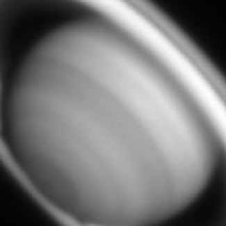
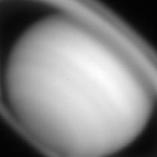
Figure 2: Saturn images taken with AImS at three different wavelengths : 727.6 nm (top left), 747.4 nm (top right) and 891.3 nm (bottom center). Saturnian north is to the upper right, and west longitudes increase towards the left side of each image. The 727.6- and 747.4-nm images were obtained about UT 7:00 February 8, 2002, and the 891.3-nm image was taken around 30 minutes later.

3.2 Geometric calibration

We fit the limb and ring profiles of each image to define the surface coordinates on Saturn. This process maps a latitude-longitude grid onto the x-y images of Saturn by using calculated ephemerides, plate scale, ellipsoidal planetary model and polar orientation information. A least-squares limb-fitting procedure was used to calculate the exact position of Saturn’s center on each image. The formal error in the limb-fitting algorithm yielded the planet center location to within an accuracy of about $\pm$ 0.5 pixel. Since the limb model does not account for changes in the atmospheric seeing, the true accuracy of the planet center determination is slightly worse ($\pm$ 1 pixel). This adds another $2$% of error to the model intensity computation. As a result, we adopt an uncertainty of 7%, which consists of 5% photometric uncertainty and 2% image navigation error, in the comparison between the observed intensities and model computations.

In this paper, we chose the equatorial region (planetographic latitude of $-10^{\circ}$) for detailed modeling. The relative longitude of the sampled region ranges from -$60^{\circ}$ to +$60^{\circ}$ from the central meridian, accounting for approximately 16 arcsec spanning roughly 200 pixels on our detector. We selected 60 data points from the region to obtain limb-darkening profiles at selected wavelengths. The cosines of solar and Earth zenith angle at each pixel ($\mu_{0}$ and $\mu$, respectively) are always larger than 0.4. This guarantees that the plane-parallel approximation is valid in the model intensity computation.

4 Principle of center-limb analysis and Wavelength selection

Center-limb profile analysis is a powerful tool to study the vertical structure of an atmosphere. The variation of scattering geometry along the profile enables us to sense the optical thickness and altitude of aerosol layers. Center-limb profiles at methane band centers contain aerosol information of only the highest region of the atmosphere because the strong absorption hinders deep penetration of the light into the atmosphere. Profiles in weaker absorption bands and continua contain information of the deeper atmosphere. Thus, examining center-limb profiles at different wavelengths of different absorption strength is equivalent to ’peeling off’ atmospheric layers one by one to determine the vertical cloud structure. From the wide spectral range of our entire data sets, we selected two clusters of wavelengths around the 727- and 890-nm methane bands. The reason is two-fold : 1) this selection minimizes the effect of the gaseous Rayleigh scattering, which becomes significant at shorter wavelengths, 2) the 619-nm methane absorption is too weak to create any physically meaningful contrast between the band center and nearby continuum under our total calibration error.

The variation in sampled depths as a function of wavelength is nicely visualized with contribution functions. The peak position of a contribution function illustrates where a major fraction of scattering occurs in a cloudless atmosphere at a certain wavelength. In other words, the peak location shows the altitude to which the center-limb profile of a chosen wavelength can have high sensitivity to the existence of scattering aerosols, provided there is no large aerosol opacity at higher altitudes. Therefore, when there are a number of observations at different wavelengths, narrowly-spaced contribution function peaks signify high vertical sampling resolution. However, on account of observational errors and variable image quality, it is difficult to select a set of wavelengths whose contribution function peaks are narrowly and evenly spaced. In our case, given our 7% uncertainty in the calibrated intensities, it was necessary to select the wavelengths where the observed intensities at a certain position on the Saturnian disk differ from one another by more than that amount. Bearing this argument in mind, we selected four wavelengths (726.5, 732.1, 735.8 and 747.4 nm) around the 727-nm methane band, and five wavelengths (891.3, 899.6, 906.2, 914.9 and 939.3 nm) around the 890-nm band to maximize the vertical resolution under our calibration uncertainty. These nine selected wavelengths span from the band centers to the adjacent continua as shown in Fig. 3. Hereafter, we refer to the former group of data as the ’727-nm data set’, and the latter as the ’890-nm data set’.

Figure 3: The spectral positions of our images between 700 and 950 nm. The data points were taken from the equatorial region at $-10^{\circ}$ planetographic latitude at the central meridian. The error bars represent 7% calibration error at the nine selected wavelengths in our modeling analysis.

The locations of the contribution function peaks at our selected wavelengths are displayed in Fig. 4. They were computed following the formulation of Banfield et al. (1996) and using the temperature profile of Lindal et al. (1985), under the assumption of a single-scattering cloudless atmosphere and vertical solar incidence. Though the single-scattering assumption may be inappropriate in weak methane bands and continuum, the obtained peak positions still show the approximate pressure levels at which the major fraction of scattering occurs. In the absence of aerosols, our 727- and 890-nm data sets can probe down to roughly 5- and 10-bar depths, respectively.

Figure 4: (a)(Top): Distribution of contribution functions in the 727-nm data set. (b)(Bottom): Distribution of contribution functions in the 890-nm data set. The listed wavelengths are all in units of nm.

To analyze the center-limb profiles, we employ a forward modeling approach. We construct a cloud structure model and compute synthetic center-limb profiles at the selected wavelengths using a radiative transfer code. The model profile in a strong absorption band should be affected only by the uppermost part of the model, while that in a weaker band or continuum is affected by a broad altitude range of the model structure. Thus, the model that can simultaneously reproduce a set of different observed profiles within the calibration uncertainty is considered to represent the vertical distribution of aerosols in Saturn’s atmosphere.

5 Modeling

5.1 Modeling Overview and Uniqueness of our Trial

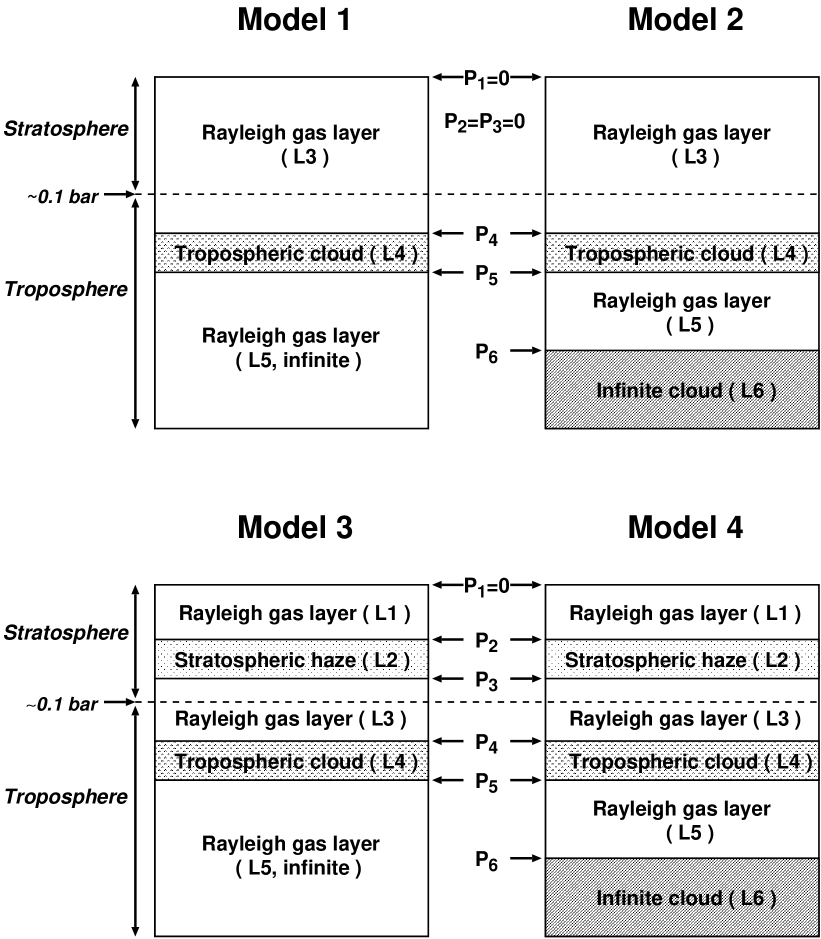
Figure 5: Four different cloud models used in our modeling process.

When we prepared our cloud structure models, we paid attention to the lessons learned from the current debate about the existence of a thick tropospheric cloud in the Jovian atmosphere. Before the entry of the Galileo Probe into the Jovian atmosphere, researchers commonly assumed the existence of a cloud of ammonium hydro-sulfide or water in the lower Jovian troposphere (at 2–5 bar level) in their cloud structure modeling, relying on the thermo-chemical prediction by Weideschilling and Lewis (1973) and infrared data analyses (Marten et al. 1981, Bézard et al. 1983, Carlson et al. 1993,1994). Nonetheless, the Galileo Probe discovered a strong depletion in water in comparison with the solar abundance ratio and detected no significant cloud opacity below 2-bar level during its decent in a region known as a ’hot spot’. Although these hot spots are known to be relatively dry and cloud-free, this surprising fact called into question the presence of a thick cloud in the Jovian lower troposphere. Recently, Sromovsky and Fry (2002) pointed out that it is possible to reproduce the optical center-limb profiles of the Jovian hot spots without any cloud below 1.2-bar level. Since modeling approaches with a thick cloud placed at the bottom were commonly adopted in previous Saturnian center-limb analyses, we now think it is necessary to try new type of Saturnian cloud models without the thick bottom cloud.

We thus set up four different types of cloud structure models, as shown in Fig. 5. These represent the existence of a stratospheric haze layer (models 3 and 4) or the no-haze case (models 1 and 2), as well as the existence of a lower infinite cloud (models 2 and 4) or the no-infinite-cloud case (models 1 and 3). The most significant point to consider is whether or not an infinite cloud at the bottom is needed in the deep atmosphere to reproduce the observed profiles. There are at most six layers within these four cases; the top Rayleigh gas layer ($\equiv$ Layer 1, L1), a stratospheric haze layer ($\equiv$ Layer 2, L2), a middle Rayleigh gas layer ($\equiv$ Layer 3, L3), an upper tropospheric cloud layer ($\equiv$ Layer 4, L4), a lower Rayleigh gas layer ($\equiv$ Layer 5, L5) and a lower infinite cloud layer ($\equiv$ Layer 6, L6). All the Rayleigh gas layers are aerosol-free. The stratospheric haze layer and upper cloud layer can be either of aerosols only or a mixture of Rayleigh gas and aerosols, depending on the initial assumptions and modeling results. The bottom infinite cloud does not contain any Rayleigh gas component. For simplicity, we sometimes refer to the stratospheric haze as ’haze’, and the upper and lower tropospheric clouds as ’UCLD’ and ’LCLD’, respectively.

In these models, $P_{1}(\equiv 0)$ is the pressure level of the atmosphere top. $P_{2}$ and $P_{3}$ signify the levels of the stratospheric haze top and bottom, respectively. $P_{4}$ and $P_{5}$ denote the levels of the top and bottom of the upper tropospheric cloud, and $P_{6}$ is defined as the top of the lower infinite cloud. The pressure difference between the top and bottom of a layer is denoted as $DLP$. For example, $DLP1$ is the pressure difference between the top and bottom of L1, so $DLP1\equiv P_{2}-P_{1}$. Similarly, $DLP2\equiv P_{3}-P_{2}$, $DLP3\equiv P_{4}-P_{3}$, $DLP4\equiv P_{5}-P_{4}$ and $DLP5\equiv P_{6}-P_{5}$. In the actual modeling computation, these $DLP$ values are treated as free variables rather than the $P$ values.

In models 1 and 2, we do not assume the existence of the stratospheric haze, hence $P_{1}=P_{2}=P_{3}=0$. In models 1 and 3, the lower Rayleigh gas layer (L5) is assumed to be infinite ($DLP5=9999.$). The LCLD in models 2 and 4 is given infinite aerosol optical thickness ($\tau_{lcld}=999$). Furthermore, we later sub-divide these four models according to the types of scattering phase functions employed in different aerosol layers. Among those models, we try to find the one that can best reproduce the observed center-limb profiles within our calibration uncertainty. The theory to calculate the optical thickness and effective single-scattering albedo of each layer is summarized in Appendix B.

We point out three advantages of our data acquisition and modeling approach. Since the AOTF camera provides 2D images at higher spectral resolution around methane bands than that of traditional narrow-band filters, we are able to investigate the entire southern hemisphere of Saturn with higher vertical sampling resolution than before. Moreover, the wide spectral range of AImS enables us to study the cloud structure at different absorption bands. This allows us to examine the wavelength dependence of the optical aerosol properties, yielding important information concerning the size distribution and composition of Saturn’s aerosols. In addition, our computational algorithm constrains free model parameters more rigorously than before. Previously, center-limb profiles of different wavelengths were fit one by one, adjusting only a few variables of strong influence on the chosen profile (e.g. varying only aerosol albedos in continuum fit). Obviously, this technique ignores the mutual dependencies among different variables. In contrast, we do not have this problem because our code simultaneously fits a set of selected profiles and returns a complete set of several fit parameters.

5.2 Selection of Gas and Aerosol Scattering Phase Functions

There is some flexibility in the choice of scattering phase functions for the aerosol layers. Typically, the two-term Henyey-Greenstein function (hereafter, TTHGF) derived from the Pioneer observations is used to simulate the scattering of the thick tropospheric cloud of Saturn (Tomasko and Doose 1984, Karkoschka and Tomasko 1992, Ortiz et al. 1996). This function has the following form:

$$P(\theta)=f\cdot P(g_{1},\theta)+(1-f)\cdot P(g_{2},\theta)$$ (1)

and

$$P(g,\theta)=\frac{1-g^{2}}{(1+g^{2}-2g\cos\theta)^{\frac{3}{2}}}$$ (2)

where $\theta$ denotes scattering angle, $f$ (0$\leq f\leq$1) is the fraction of forward-scattered light, $g_{1}$ (0$\leq g_{1}\leq$1) is the asymmetry factor of forward-scattering and $g_{2}$ (-1$\leq g_{2}\leq$0) is the asymmetry factor of back-scattering. A larger value of $g_{1}$ gives a sharper forward-scattering peak, while a larger absolute value of $g_{2}$ gives a sharper back-scattering peak. The TTHGF obtained by Tomasko and Doose (1984) in red light in the southern Saturnian equatorial region (from $-7^{\circ}$ to $-11^{\circ}$) ([$f,g_{1},g_{2}$]=[0.763, 0.620, -0.294]) is used as the scattering phase function of the lower tropospheric cloud throughout our modeling. For the stratospheric haze and UCLD, we use both the above TTHGF of Tomasko and Doose (1984) and Mie scattering phase functions of different aerosol size distributions. The modified gamma function (Hansen and Travis 1974), which is defined by two parameters, effective radius $a$ and effective variance $b$, was employed to simulate the particle size distribution. The average Mie phase function for a given size distribution was obtained by weighting and adding up Mie phase functions of different aerosol sizes. For the purpose of Mie computation for a certain particle size, we adopted the code of Bohren and Hoffman (1983). The adopted parameters in the Mie scattering computation are listed in Table 1.

Applied layer	$a$	$b$	$n_{r}$
Stratospheric haze	0.15	0.1	1.43
Upper tropospheric cloud	1.50	0.1	1.43

Table 1: List of Mie scattering parameters used in our modeling. $a$ is the effective aerosol radius in $\mu$m, and $b$ is the effective variance of Hansen’s size distribution function (Hansen and Travis 1974). $n_{r}$ represents the real refractive index of aerosols.

The values listed in Table 1 were employed because they were used in previous publications (Karkoschka and Tomasko 1993, Ortiz et al. 1996) and facilitate the comparison between our results and previous work. The photochemically expected condensates in the Saturnian stratosphere include diacetylene ($C_{4}H_{2}$, $n_{r}=1.42$) and ethane ($C_{2}H_{6}$, $n_{r}=1.44$) (Karkoschka and Tomasko 1993). Therefore we adopt the average of those indices as the refractive index for our haze layer. The refractive index of the UCLD is assumed to be that of ammonia ice. We assume the imaginary part of aerosol refractive index ($n_{i}$) is zero. Instead, absorption by aerosols is taken into account by adjusting the single-scattering albedo of aerosols in the modeling process. With these particle parameters, we generated the Mie phase functions at 730 and 900 nm, and applied them to the 727-nm data set and the 890-nm data set, respectively.

At this point, we sub-divided the 4 main models into 12 models, depending on the phase functions adopted in the haze and UCLD layers (Table 2). We refer to the adopted TTHGF as ’H-G (red)’, the Mie function for the haze as ’Mie 0.15’ and the Mie function for the UCLD as ’Mie 1.5’.

Table 2: Cloud models with different phase functions ($P(\theta)$)

Parent Model	Model #	Haze $P(\theta)$	UCLD $P(\theta)$	LCLD $P(\theta)$
1	1-1	N.A.	H-G (red)	H-G (red)
	1-2	N.A.	Mie 1.5	H-G (red)
2	2-1	N.A.	H-G (red)	H-G (red)
	2-2	N.A.	Mie 1.5	H-G (red)
	3-1	H-G (red)	H-G (red)	H-G (red)
3	3-2	H-G (red)	Mie 1.5	H-G (red)
	3-3	Mie 0.15	H-G (red)	H-G (red)
	3-4	Mie 0.15	Mie 1.5	H-G (red)
	4-1	H-G (red)	H-G (red)	H-G (red)
4	4-2	H-G (red)	Mie 1.5	H-G (red)
	4-3	Mie 0.15	H-G (red)	H-G (red)
	4-4	Mie 0.15	Mie 1.5	H-G (red)

The scattering phase function in the Rayleigh gas layers is that of Rayleigh scattering ($P_{R}(\theta)$):

$$P_{R}(\theta)=\frac{3}{4}(1+cos^{2}\theta)$$ (3)

where $\theta$ again denotes scattering angle. In the cases where aerosols and Rayleigh gas co-exist in a layer, we assume that they are uniformly mixed and adopt the aerosol’s phase function since the opacity by the Rayleigh scattering ($\tau_{R}$) was always negligibly small compared with the aerosol opacity ($\tau_{A}$) due to the relatively long wavelength of our observations in any layer ($\tau_{R}/\tau_{A}<10^{-3}$). All the phase functions adopted in our modeling are illustrated in Fig. 6.

Figure 6: Different phase functions used in our modeling.

5.3 Atmospheric Composition and Methane Absorption

With respect to the atmospheric composition, a number of different results have been published (Hanel et al. 1981, Conrath et al. 1984, Courtin et al. 1984, Atreya et al. 1999, Conrath and Gautier 2000, Atreya et al. 2003). We chose the values of Hanel et al. (1981) for the Saturnian hydrogen and helium abundance and assumed that the methane mole fraction is 0.002 (Table 3). These are identical to those used by Stam et al. (2001), and nearly equal to those used in other cloud modeling efforts (Tomasko and Doose 1984, Karkoschka and Tomasko 1992, 1993, Ortiz et al. 1996, Acarreta and Sánchez-Lavega 1999). Therefore, this choice also facilitates comparison between our results and previous studies.

Table 3: Atmospheric composition of Saturn assumed in our modeling.

Gas Species	Mole fraction
$H_{2}$	0.940
$He$	0.058
$CH_{4}$	0.002

There are several publications that address the methane absorption coefficients. Through the analysis of the spectra of giant planets, Karkoschka (1994) reported that the optical methane band shapes are narrower and band peaks are deeper at colder temperatures in giant planets’ atmospheres than at room temperatures. The newest laboratory measurements of methane absorption coefficients at 77 K (Singh and O’Brien 1995, O’Brien and Cao 2002) showed very good agreement with Karkoschka’s result. Unfortunately, the data sets of those new laboratory measurements do not fully cover the wavelength ranges in either our 727- or 890-nm data sets. Therefore, we employ the methane coefficient values derived by Karkoschka (1994) in this paper. In our computations, these values were convolved with the transmission function of the AOTF filter to obtain the effective value at each selected passband (Table 4).

Table 4: Effective methane absorption coefficients ($k_{\mbox{\tiny$CH_{4}$}}$ in [km–am$]^{-1}$) for our wavelengths of interest ($\lambda$ in [nm]).

$\lambda$	$k_{\mbox{\tiny$CH_{4}$}}$
726.5	3.863
732.1	1.653
735.8	0.690
747.4	0.015
891.3	24.471
899.6	12.699
906.2	2.277
914.9	0.860
939.3	0.021

5.4 Free and fixed parameters

The following 11 parameters are left undetermined:

• Aerosol opacities in L2 ($\equiv\tau_{haze}$) and L4 ($\equiv\tau_{ucld}$)

• Aerosol single-scattering albedos in L2 ($\equiv\varpi_{0,haze}$), L4 ($\equiv\varpi_{0,ucld}$) and L6 ($\equiv\varpi_{0,lcld}$)

• Rayleigh scattering albedo at continua

• Physical thickness of L1 – L5 ($DLP1$ – $DLP5$).

These parameters must be fixed by further assumptions or determined from the center-limb profile fitting. We set the continuum Rayleigh scattering albedo to 1.0, considering no gas absorption other than that of methane. In addition, we fixed the physical thickness of the haze layer. According to Karkoschka and Tomasko (1993), the optical thickness of the stratospheric haze is always very small, near $0.2$ at 340 nm, when the pressure difference between the top and bottom of the stratospheric haze ($DLP2$) is roughly 100 mb. In the spectral region of our data sets (726 – 940 nm), this opacity would be even smaller when we consider the likely particle size ($\sim 0.15$ $\mu$m) of the haze (Karkoschka and Tomasko 1993). From this argument, we assume that variation in $DLP2$ has only a minor effect on the computation result and therefore adopt the value 10 mb for $DLP2$. All the other pressure variables are left as free variables; the danger of assuming a certain pressure level for any cloud deck is well explained by Sromovsky and Fry (2002) and others for the case of the Jovian atmosphere.

In the end, we are left with at most 9 free variables ($\tau_{haze}$, $\varpi_{0,haze}$, $\tau_{ucld}$, $\varpi_{0,ucld}$, $\varpi_{0,lcld}$, $DLP1$, $DLP3$, $DLP4$, $DLP5$) to be adjusted to reproduce the observed center-limb profiles.

5.5 Optimization procedure and initial conditions

5.5.1 Optimization procedure

To examine the wavelength dependence of aerosol opacity and albedo, our fitting operations for the 727- and 890-nm data sets were done individually. First, we fit the 890-nm data set to determine the entire cloud structure because the 890-nm data set more strictly constrains the model with the wider altitude coverage and more wavelengths. Then, from the best-fitting parameters of the 890-nm data set, we adopt the pressure levels of aerosol layers and fix these parameters in the subsequent 727-nm data set simulations. We then obtain aerosol opacities and albedos near 727 nm. Thus, in addition to the cloud structure, we can determine the wavelength dependence of optical properties of aerosols.

The intensity computation was done with a radiative transfer code based on the adding-doubling method (Hansen 1969). The accuracy of fitting for each data set is judged by the following reduced $\chi^{2}$.

$$\chi^{2}=\frac{1}{N_{free}}\sum_{i}\displaystyle{\frac{((I/F)_{i,obs}-(I/F)_{i,com})^{2}}{\sigma_{i,obs}^{2}}}$$ (4)

where

$$N_{free}=N_{points}-N_{variable},$$ (5)

$(I/F)_{i,obs}$ :

Observed $I/F$ value at i th data point,

$(I/F)_{i,com}$ :

Computed $I/F$ value at i th data point,

$\sigma_{i,obs}$ :

Observational error of $I/F$ at i th data point,

$N_{free}$ :

Degree of freedom of the fit,

$N_{points}$ :

Number of data points of a profile,

$N_{variable}$ :

Number of variables used in fitting a profile.

Numerically, a solution is considered acceptable if the $\chi^{2}$ is smaller than 1.0.

We search multi-dimensional parameter space (up to 9 dimensions) for the optimum combination of parameter values that can simultaneously fit a certain number of profiles in a given data set (five in the 890-nm data set and four in the 727-nm data set) within our calibration error. This is equivalent to seeking the minimum point of $\chi^{2}$. To do this, our code follows the gradient-expansion method in Bevington and Robinson (1992). Given an initial set of parameters, this method computes the gradient of $\chi^{2}$ at that point in the multi-variable space, and takes the next point of smaller $\chi^{2}$ along the gradient vector. This process is iterated until a ’hollow’ of $\chi^{2}$ is found. However, the well-known difficulty is that the discovered hollow point may be just one of the local-minimum points of $\chi^{2}$, regardless of the adopted optimization method. The only way to avoid this concern is to cover the entire parameter space with a fine grid and adopt grid-search method, though the huge computational burden makes this approach impractical. Therefore, a good initial setting is essential to reach the correct minimum point in our modeling. Nevertheless, since there is not enough information available to make reasonable presumptions about desirable initial parameters, our initial settings must cover as wide a range as possible in the parameter space. Due to this requirement, we integrated the grid-search algorithm into our code so that our initial conditions can systematically explore the vast parameter space within their physically reasonable range. Namely, we set up a grid in the multi-parameter space and let all the grid-points represent our initial conditions for optimization.

In practice, for a chosen type of model, we specify a large number of combinations of reasonable initial values. Starting from each of those initial conditions, our computer program finds a local minimum point of $\chi^{2}$ and records it as a solution for the given initial condition. Among those recorded solutions, we choose the one that gives the smallest $\chi^{2}$ for the chosen cloud model. The same procedure is used for all the different cloud models to obtain a model-specific solution for each cloud model. After examining and comparing those model-dependent solutions, we finally choose the true best-fit result for the given data set of Saturn.

5.5.2 Initial conditions and their limitations

Table 5: The minimum, maximum and initial values of free variables. All the $DLP$ values are in units of bar.

Free Variable (if it exists)	Min.	Max.	Initial values
$\tau_{haze}$	0.	0.5	0.1
$\tau_{ucld}$	0.	50.	1., 5., 10., 30.
$\varpi_{0,haze}$	0.95	1.0	0.975, 0.995
$\varpi_{0,ucld}$	0.95	1.0	0.975, 0.995
$\varpi_{0,lcld}$	0.95	1.0	0.975, 0.995
$DLP1$	0.	0.1	0.05
$DLP3$	0.	10.	0.1, 0.5, 1., 3.
$DLP4$	0.	20.	0.1, 0.5
$DLP5$	0.	9999.	0.1, 0.5, 1. 3.

The minimum, maximum and initial values of the free variables in our modeling are summarized in Table 5. The maximum value of $\tau_{haze}$ is set to 0.5 because the haze opacity should be small based on the argument of Karkoschka and Tomasko (1993). $\tau_{ucld}$ is one of the most important parameters in our modeling. Therefore, we allow it to have a large range of possible values. The maximum of $\tau_{ucld}$ is practically infinite ($\tau_{ucld}=50.$), and four different initial values are given spanning 1 – 30. In light of previous modeling results (Tomasko and Doose 1984, Karkoschka and Tomasko 1992,1993, Ortiz et al. 1996, Acarreta and Sánchez-Lavega 1999), all aerosol albedos ($\varpi_{0,haze}$, $\varpi_{0,ucld}$ and $\varpi_{0,lcld}$) are limited between 0.95 and 1.0. They are assigned one of two possible initial values, 0.975 and 0.995, to represent either an absorbing or a reflective case.

$DLP1$ controls the altitude of the stratospheric haze. Hence, its upper limit is 0.1 bar, which corresponds to the entire stratosphere. The gap between the haze and UCLD is given by $DLP3$. Here, we chose the maximum value of 10 because $DLP3$ value cannot exceed this and still reproduce the observed intensity at strong absorption bands when there is only a thin haze layer above the UCLD. Since this is an important parameter for the 727-nm data fit, we use four initial values. Another important parameter, especially in the model group 1, is the thickness of the UCLD, $DLP4$. The maximum of this variable is allowed to be 20, which includes the extreme case where the UCLD is an aqueous $H_{2}O-NH_{3}$ cloud extending up to the stratosphere. Only two small initial values are used for $DLP4$ because we initially suppose that the UCLD is not physically very thick. The vertical ’distance’ between the UCLD and LCLD is determined by $DLP5$. The maximum is set to 9999., which means there is no LCLD. The four initial values of $DLP5$ take into consideration all the cases where the LCLD has a major and minor contribution to the outgoing radiation.

In the model group 1, the free parameters are $\tau_{ucld}$, $\varpi_{0,ucld}$, $DLP3$ and $DLP4$. Thus, 64 (= $4\times 2\times 4\times 2$) types of initial conditions are used. In the model group 2, the free variables are $\tau_{ucld}$, $\varpi_{0,ucld}$, $\varpi_{0,lcld}$, $DLP3$, $DLP4$ and $DLP5$. They have 512 (= $4\times 2\times 2\times 4\times 2\times 4$) types of initial value sets. In the model group 3, $\tau_{haze}$, $\tau_{ucld}$, $\varpi_{0,haze}$, $\varpi_{0,ucld}$, $DLP1$, $DLP3$ and $DLP4$ are adjusted. This corresponds to 128 (= $1\times 4\times 2\times 2\times 1\times 4\times 2$) types of initial conditions. In the model group 4, all the nine parameters in Table 5 are adjusted to fit the profiles, and a total of 1024 (= $1\times 4\times 2\times 2\times 2\times 1\times 4\times 2\times 4$) types of initial conditions are tested. In the end, we explored a total of 5760 different initial conditions for the 890-nm data fitting and obtain the same number of corresponding solutions. The subsequent 727-nm data fitting used a total of 240 initial conditions. The entire computation process took about 70 hours on a 2.8 GHz Pentium workstation. By examining those numerous solutions, we determined the best-fit cloud model for Saturn’s equatorial region over 726 – 940 nm.

5.6 Radiative Transfer code check

Our adding-doubling code was originally written for the analysis of Pioneer 10 and 11 data. It has a total of 22 quadrature points for the integration over the scattering angles and can hold up to 60 Fourier azimuthal expansion terms. We checked the accuracy of this code using several types of scattering phase functions.

5.6.1 Simple phase functions

First, we tested the computation accuracy using simple phase functions. The simplest isotropic scattering case was tested in comparison with the analytic solutions of Chandrasekhar (1960). A Rayleigh scattering case was also examined following the method of Stammes et al. (1989). With the phase functions of Jupiter’s cloud and haze, we cross-matched our computational intensities with those of Dr. T. Satoh (private communication). Throughout these procedures, the agreement was excellent ($\leq 0.5\%$) and therefore we are confident that our simulation is sufficiently accurate when the above phase functions are employed. We also compared our results with those obtained using the DISORT code that is based on the Discrete Ordinate Method (Stamnes et al. 1988, Thomas and Stamnes 1999). This method is conceptually very different from the Adding-Doubling method to solve radiative transfer problems, as concisely described by Hansen and Travis (1974). In the DISORT computation, 3 streams were taken for the isotropic and Rayleigh scattering cases, and 32 or higher was used for other cases. Again, the agreement was nearly perfect (deviation $\leq 0.1\%$) with the use of the above phase functions and the Saturnian TTHGFs.

5.6.2 Mie phase function

Our concern regarding the Mie scattering case was that the sharp forward scattering lobes seen in Mie phase functions would not be accurately included in our computation. Benassi et al. (1984) was referred to for the accurate computational results with highly asymmetric Mie phase functions.

The accuracy of our computations deteriorated when the effective aerosol radius reached about 10 $\mu$m and the corresponding forward scattering lobe became too sharp (the normalized functional value is $10^{3}$ – $10^{4}$ at $\theta=0^{\circ}$). This is probably because the quadrature points of our code are not distributed finely enough to accurately integrate a very sharp forward scattering peak. On these occasions we followed the truncation method of Potter (1970), in which the forward-scattered light in the diffraction peak is regarded as unscattered. This operation results in a significant reduction in scattering cross section of aerosols, and therefore we need to appropriately re-scale aerosol opacities and albedos. This truncation dramatically improved our computational accuracy in the large particle cases. The deviation from the published values in Benassi et al. (1984) was less than 1% in most cases, though there were a few cases where the deviations were as large as $\sim 3\%$.

Fortunately, with the particle sizes employed in our Saturnian modeling computations ($a$ = 0.15 and 1.5), no truncation was necessary because the Mie phase functions were smooth enough in those cases. Compared with a 64-stream DISORT result, the computational error was smaller than 0.06% for $a$=0.15 and smaller than 0.3% for $a$=1.5. These deviations are totally negligible in our modeling.

6 Results and Discussion

The fitting accuracies for all of our models are shown in Table 6.

Table 6: Equatorial profile fitting result

Model	Best 5 $\chi^{2}$ in 890-nm data set	Best 5 $\chi^{2}$ at 939.3 nm	Best $\chi^{2}$ in 727-nm data set
1-1	0.177 – 0.193	0.33 – 0.43	0.107
1-2	0.402 – 0.441	0.86 – 1.12	-
2-1	0.149	0.30	0.437
2-2	0.297 – 0.298	0.80 – 0.81	-
3-1	0.192 – 0.240	0.34 – 0.55	0.082
3-2	0.261 – 0.488	0.45 – 0.93	-
3-3	0.186 – 0.299	0.32 – 0.95	0.079
3-4	0.222 – 0.313	0.39 – 0.65	-
4-1	0.151 – 0.153	0.30 – 0.31	0.251
4-2	0.179 – 0.185	0.40 – 0.41	-
4-3	0.139 – 0.144	0.23 – 0.25	0.098
4-4	0.160 – 0.162	0.29 – 0.31	0.095

6.1 890-nm data set fitting

In our fitting of the 890-nm data set, we obtained a number of different solutions derived from various initial conditions based on our cloud models. The $\chi^{2}$ values for the entire data set are well smaller than 1 and very close to one another for each assumed model, making it difficult to choose the best among them if we use the $\chi^{2}$ alone. Therefore, we first selected the five best solutions for each model. The main deviation source of this 890-nm data set is the flattened profile shape from the central meridian towards the dusk limb (of negative relative longitude) of the 939.3-nm profile, as shown in Fig. 7. This discrepancy becomes more prominent as wavelength increases from 891.3 nm (Fig. 8). As a result, the fitting residual of this 939.3-nm profile dominates the overall fitting accuracy. For this reason, we use the $\chi^{2}$ value at 939.3 nm as an additional criterion for assessing the fitting accuracy for this data set. In Table 6, the degradation of 939.3-nm fit is obvious when the UCLD adopts the ’Mie 1.5’ phase function. In that case, the reproduced limb-darkening becomes steep and the computed intensity tends to be low at the both limbs, presumably because of the strong forward scattering of the UCLD. This trend is the most evident when there is no haze layer above the UCLD (e.g. models 1-2 and 2-2). The comparison between the results of model 1-1 and 1-2 clearly illustrates this effect (Fig. 7). Therefore, the average tropospheric particle size smaller than 1.5 $\mu$m is preferred in our models.

Figure 7: Plot of the 939.3-nm profile and comparison of best-fit results at 939.3 nm between model 1-1 and 1-2. The error bars show $\pm$7% of calibration error.

To proceed to the 727-nm data fitting, we selected only the models that satisfy the following two conditions : i) $\chi^{2}$ at 939.3 nm must be smaller than 0.4, ii) $\chi^{2}$ for overall 890-nm data set must be smaller than 1.2 times the best $\chi^{2}$ in the model group to which the considered model belongs. The first condition is adopted because the systematic deviation between the computed and observed 939.3-nm profiles becomes visually clear when this value exceeds 0.4. The second condition is set rather empirically and arbitrarily as a constraint on the fitting at the other wavelengths. This 20% range of $\chi^{2}$ corresponds to the difference in the best $\chi^{2}$ between models 3-3 and 3-4 or between models 4-2 and 4-3. The reason we apply this second condition only within each model group is that we examine the dependence of solutions on assumed cloud models. As a consequence of the above two criteria, the solutions from models 1-1, 2-1, 3-1, 3-3, 4-1, 4-3 and 4-4 remain qualified as best-fit for Saturn’s equatorial atmospheric structure near 890 nm. Next, we fit the 727-nm data set using these qualified cloud models.

6.2 727-nm data set fitting

We fit the 727-nm data set using the cloud layer altitudes of the qualified models obtained through the 890-nm data fitting. The best results are shown again in Table 6. In this data set, the dawn-dusk asymmetry is weaker than in the 890-nm data set, hence the smaller residual $\chi^{2}$ for the best-fit results.

It is clear from an examination of Table 6 that models 2-1 and 4-1 should be discarded on account of their significantly poorer fitting accuracy than the others. Consequently, seven solutions from five different models (one solution from each of model 1-1, 4-3 and 4-4, and two from each of 3-1 and 3-3) remain. These solutions are described in Table 7, and displayed graphically in Fig. 9. The two solutions from each of model 3-1 or 3-3 are derived from different initial conditions. The uncertainties in Table 7 correspond to a 20% of increase in $\chi^{2}$. We allowed this $\chi^{2}$ range to be consistent with the argument of criterion-setting in the preceding section. These parameter uncertainties quantify how sensitively the fitting accuracy depends on different variables.

Table 7: Best-fit modeling results for the equatorial region of Saturn. (a)(Top): Solutions without LCLD. (b)(Bottom): Solutions with LCLD.

Variables	1-1	3-1 (1)	3-1 (2)	3-3 (1)	3-3 (2)
$\chi^{2}_{890}$	0.193	0.192	0.205	0.186	0.191
$\tau_{haze,890}$	-	0.00$+$0.18	0.21$\pm^{0.24}_{0.12}$	0.31$\pm^{0.19}_{0.05}$	0.27$\pm^{0.23}_{0.07}$
$\tau_{ucld,890}$	16.97$\pm^{5.53}_{1.71}$	14.82$\pm^{4.97}_{1.00}$	39.42$\pm^{10.56}_{3.43}$	47.66$\pm^{2.31}_{3.68}$	49.81$\pm^{0.15}_{3.06}$
$\varpi_{0,haze,890}$	-	1.000$-$0.050	1.000$-$0.018	1.000$-$0.010	1.000$-$0.012
$\varpi_{0,ucld,890}$	0.998$\pm^{0.002}_{0.001}$	0.998$\pm$0.001	0.997$\pm^{0.002}_{0.001}$	0.997$\pm^{0.002}_{0.001}$	0.997$\pm^{0.002}_{0.001}$
$\varpi_{0,lcld,890}$	-	-	-	-	-
$\chi^{2}_{727}$	0.107	0.102	0.082	0.079	0.082
$\tau_{haze,727}$	-	0.12$\pm^{0.09}_{0.11}$	0.01$\pm^{0.18}_{0.01}$	0.00$+$0.34	0.00$+$0.23
$\tau_{ucld,727}$	8.87$\pm^{0.65}_{0.53}$	8.407$\pm^{0.42}_{0.45}$	19.12$\pm^{1.54}_{3.94}$	19.55$\pm^{3.17}_{4.49}$	27.03$\pm^{2.38}_{6.87}$
$\varpi_{0,haze,727}$	-	0.950$+$0.030	0.968$\pm^{0.032}_{0.018}$	0.997$\pm^{0.003}_{0.047}$	0.989$\pm^{0.011}_{0.039}$
$\varpi_{0,ucld,727}$	0.999$\pm$0.001	1.000$-$0.001	0.997$\pm$0.001	0.996$\pm^{0.002}_{0.001}$	0.996$\pm$0.001
$\varpi_{0,lcld,727}$	-	-	-	-	-
$DLP1$	-	0.004$\pm^{0.003}_{0.004}$	0.010$\pm^{0.002}_{0.009}$	0.018$\pm^{0.002}_{0.008}$	0.021$\pm^{0.002}_{0.007}$
$DLP3$	0.024$\pm^{0.004}_{0.007}$	0.010$\pm^{0.003}_{0.007}$	0.014$\pm^{0.003}_{0.011}$	0.016$\pm^{0.002}_{0.014}$	0.003$\pm^{0.002}_{0.003}$
$DLP4$	0.269$\pm^{0.031}_{0.072}$	0.240$\pm^{0.017}_{0.072}$	0.515$\pm^{0.049}_{0.163}$	0.512$\pm^{0.043}_{0.174}$	0.719$\pm^{0.046}_{0.297}$
$DLP5$	-	-	-	-	-

Variables	4-3	4-4
$\chi^{2}_{890}$	0.144	0.162
$\tau_{haze,890}$	0.50$-$0.08	0.50$-$0.07
$\tau_{ucld,890}$	5.17$\pm^{1.36}_{0.38}$	9.30$\pm^{2.08}_{0.80}$
$\varpi_{0,haze,890}$	1.000$-$0.008	1.000$-$0.009
$\varpi_{0,ucld,890}$	1.000$-$0.001	1.000$-$0.001
$\varpi_{0,lcld,890}$	0.993$\pm^{0.005}_{0.004}$	0.997$\pm$0.002
$\chi^{2}_{727}$	0.098	0.095
$\tau_{haze,727}$	0.12$\pm^{0.10}_{0.08}$	0.14$\pm^{0.20}_{0.14}$
$\tau_{ucld,727}$	4.22$\pm^{0.23}_{0.35}$	7.39$\pm^{0.39}_{0.50}$
$\varpi_{0,haze,727}$	0.950$+$0.036	1.000$-$0.025
$\varpi_{0,ucld,727}$	1.000$-$0.001	1.000$-$0.001
$\varpi_{0,lcld,727}$	0.994$\pm^{0.004}_{0.003}$	0.995$\pm^{0.002}_{0.001}$
$DLP1$	0.023$\pm^{0.002}_{0.008}$	0.022$\pm^{0.003}_{0.008}$
$DLP3$	0.024$\pm^{0.004}_{0.013}$	0.023$\pm^{0.004}_{0.012}$
$DLP4$	0.026$\pm^{0.008}_{0.019}$	0.026$\pm^{0.008}_{0.017}$
$DLP5$	0.567$\pm^{0.914}_{0.495}$	0.540$\pm^{0.840}_{0.422}$

Figure 8: Graphical display of the best-fit results listed in Table 7 at five different wavelengths around 890 nm used in our modeling. The error bars show $\pm$7% of calibration error. The solutions 3-1 (2) and 3-3 (2) are not plotted because they show no visually significant difference.

Figure 9: Same as Fig. 8 but at four different wavelengths around 727 nm.

Judging from the average $\chi^{2}$ of the two data sets, we can state that the model 4-3 solution is the best to reproduce the Saturnian center-limb profiles of the equatorial region over the entire spectral range in our observations. However, we note the following points : a) there may be systematic biases associated with the selected cloud model structures, b) the difference in $\chi^{2}$ between the model 4-3 solution and the others is too small to be significant given our calibration uncertainty. The great difficulty in determining the best solution is clearly seen when we plot the seven solutions together at all the nine wavelengths (Figs. 8 and 9). Without any more objective measures to distinguish one solution from another, we can not tell which solution best represents the real cloud structure in Saturn’s atmosphere. Therefore, though we put more stress on the model 4-3 solution, we would rather summarize some common features among the seven listed solutions than take a risk of fully relying on the ’numerically-best’ one. The drawback of this approach is that the ensuing discussion inevitably tends to be qualitative; nevertheless, the model-independent features among those solutions will give us real physical insight about the equatorial cloud structure of Saturn.

6.3 Result Overview

First, we obtain somewhat better results from the two models with infinite bottom cloud (4-3 and 4-4). This difference comes from the better fit in the 939.3-nm profile. The large uncertainties in $DLP5$ imply that this continuum intensity is not strongly affected by the LCLD altitude, as long as the LCLD top exists within the altitude range of 0.15 – 1.5 bar. Therefore, we suggest that a region of higher aerosol density located somewhere within 0.15 – 1.5-bar level is preferred to better reproduce the profile at 939.5 nm. Nonetheless, our calibration uncertainty and model-dependent behaviors of the derived solutions prevent us from determining if this high aerosol density region exists as a separated cloud deck or a part of an extended cloud. These model-dependent features are discussed in detail in the subsequent section.

We also note the narrow gap between the haze and UCLD ($DLP3$ is 10 – 24 mb for all the haze-containing solutions). Since the haze bottom level (= $DLP1+DLP2$ bar) always exists at 15 – 30 mb, this suggests that the tropospheric cloud in the Saturnian equatorial region extends up into the stratosphere.

Another noteworthy trend is the significantly smaller UCLD opacity in the 727-nm data fitting than in the 890-nm data fitting. The models without LCLD (1-1, 3-1 and 3-3) show a difference of roughly a factor of 2 in the UCLD optical thickness, and a difference of about 20% is seen in the models with the LCLD (4-3 and 4-4). This opacity variation is required from the fact that the equatorial profiles near 727 nm are relatively dark given their relatively high brightness around 890 nm. In fact, it is possible that the particle scattering efficiency becomes larger with longer wavelength over the spectral range of our data sets (700 – 950 nm), provided the particle size is in an appropriate range. Figure 10 illustrates the wavelength dependence of the scattering efficiency with various effective aerosol radii and variances of Hansen’s size distribution function.

Figure 10: Wavelength dependence of normalized scattering efficiency ($Q_{sca}$) over 700 – 950 nm with different effective aerosol radii ($a$, in $\mu$m). $Q_{sca}$ is normalized at 730 nm, and $n_{r}=1.43$. Top: $b=0.01$. Bottom: $b=0.10$.

The increase in aerosol opacity of the UCLD by roughly a factor of 2 suggests a small variance in the aerosol size distribution ($b\sim 0.01$) and an effective radius of about 0.9 $\mu$m. If we only examine the opacity increase at longer wavelengths, we can still set a lower limit of $a$ around 0.7 – 0.8 $\mu$m, if $b\sim$ 0.01 – 0.1 and $n_{r}=1.43$.

Regarding the haze parameters, we see an even more anomalous wavelength dependence. The haze optical thickness is disturbingly larger around 890 nm than around 727 nm by roughly a factor of 4 or more, except for the model 3-1 (1) case. The large fractional errors in haze opacity and albedo at both 727 and 890 nm imply that the haze is relatively unimportant for the fitting results. Furthermore, the aerosol free layer between the haze and UCLD is always very thin in our solutions. Actually, in our additional trial simulations where we fixed $DLP3$ value to zero, we could obtain solutions of very similar cloud structures and fitting accuracies. This means that the thin aerosol-free layer between the haze and the UCLD is not essential for the profile fit. Based on these arguments, we suggest that the stratospheric haze is mostly mixed with the vertically extended tropospheric cloud. The apparent existence of separate haze layers in the haze-containing solutions are regarded as mere numerical artifacts. This inference is further supported by the great similarity between the solution 1-1 and solution 3-1 (1) in terms of the fitting accuracy, UCLD albedo, UCLD top and bottom altitudes and total opacity of the haze and UCLD. Recalling that both of these two solutions adopt the common ’H-G (red)’ phase function in all the aerosol layers, we can say that those two results are practically equivalent.

A combination of ’Mie 0.15’ phase function in the haze and ’H-G (red)’ or ’Mie 1.5’ in the UCLD tends to give slightly better fits to the data, as seen in models 3-3, 4-3 and 4-4. Following the above interpretation of the upper atmospheric structure, this supports the idea that the aerosol phase function at a lower altitude of the UCLD is more forward-scattering, indicating a larger aerosol size with increasing depth. In our view, the uppermost part of the UCLD is mainly composed of very small particles ($r_{eff}\sim$ 0.15 $\mu$m) probably including some haze components, and the lower main body of the UCLD consists of larger particles between 0.7 – 0.8 and 1.5 $\mu$m.

None of our cloud models, which are all longitudinally averaged, could fit well the high dusk-side intensity near the two continuum wavelengths (e.g. 747.4 and 939.3 nm). The flat-fielding process is not likely to be the origin of this feature because it does appear in the images taken on the previous night (Feb. 7, 2002) at different west longitudes despite the different positions and orientations on the detector, where the flat-field profiles had totally different shapes along the equatorial region. Another possibility, the image navigation error, is also unlikely because the limb-fitting algorithm works better at continuum wavelengths, where the contrast between the disk and background is the highest. Therefore, the deviation from the longitudinally averaged model in the dusk limb could represent a real diurnal variation, though the deviation is not large enough compared with our calibration errors. Any conclusive statements about this phenomenon are reserved for future observations with higher photometric accuracy.

6.4 Dependence on the model structures and initial conditions

Here we discuss some noticeable dependence of fitting results on assumed cloud models and initial conditions for optimization process. Discussing and summarizing these effects provides us with valuable lessons to be kept in mind for the interpretation of the results presented herein as well as in future modeling efforts. We found that the assumption of an infinite bottom cloud and the choice of aerosol scattering phase function both strongly influence the fitting results. We also found that different initial settings for optimization can lead to very different solutions.

First, the total combined opacity of the haze and UCLD is systematically smaller if the LCLD exists. This is conceivable because the LCLD can account for some fraction of the required opacity to fit profiles in weak absorption bands and continua. Second, the physical thickness of the UCLD ($DLP4$) is much smaller in the models containing LCLD. This trend is related to the aforementioned first feature. To maintain a certain reflectivity in an absorption band with a small total aerosol opacity in upper aerosol layers, those aerosols needs to be concentrated in a narrow pressure range, resulting in a physically thin cloud. This is the main cause of the surprisingly high altitudes of the UCLD bottom in our 4-3 and 4-4 solutions, which unrealistically indicate that the whole UCLD ($\tau=5-9$) exists above the tropopause (Saturn’s tropopause is located around the 0.1-bar level). Therefore, we consider this high UCLD bottom level in those two solutions as an numerical ’illusion’ associated with the assumption of the LCLD, and conclude that a cloud in the troposphere extends into the stratosphere. Third, the gaps between aerosol layers are larger in the models with the LCLD. This is probably because the UCLD is more narrowly confined and we do not consider any gas absorption in the LCLD. Namely, the increase in gas absorption in thicker aerosol-free layers compensates for reduced absorption in physically thin clouds and LCLD. If we allow for mixing of gas in the bottom cloud, the $DLP5$ value will become smaller and the vertical structure will approach that of the solutions 3-1 or 3-3. From these discussions, we infer that the adoption of an infinite bottom cloud in a cloud model introduces: high altitude, low opacity and a small physical thickness of an upper aerosol layer, and also introduces relatively large gaps between aerosol-containing layers.

Regarding the effect of phase function, it is evident that the opacity of the UCLD is strongly influenced by the chosen type of scattering phase function when we compare the solutions of model 4-3 and 4-4. Generally, more forward-scattering aerosols tend to require more opacity to reproduce observed intensities in nearly back-scattering direction, i.e. observations at small phase angles.

The dependence on initial conditions is clear in the comparison between the solutions 3-1 (1) and 3-1 (2), and to a lesser extent between 3-3 (1) and 3-3 (2). These examples demonstrate that different initial conditions for optimization can result in very different solutions of equally good fit through simultaneous adjustment of multiple variables. What is worse, we found no apparent correlation between the initial conditions and corresponding final solutions in our analysis.

Therefore, when a forward-modeling approach is taken to analyze an atmosphere, one must : a) fix as many atmospheric parameters as possible based on reasonable assumptions or observational facts, b) be very careful about the validity of the assumptions about cloud structure model, c) try as wide a range of initial conditions as possible, and d) take great care in interpreting modeling results, recognizing the influence of the assumptions on the results.

6.5 Comparison with previous results

In this section, we compare our results with previous studies. Despite the uniqueness of our modeling method and difference in data acquisition epoch, we see some interesting similarities and differences.

In the equatorial region of Saturn, Stam et al. (2001) found the stratospheric haze bottom around 20 mb level, the UCLD top around 60 mb level and the tropospheric cloud bottom around 300 mb level by inverting the near-IR spectra of Saturn taken in August, 1995. The haze bottom level is consistent with our results ($P=14-33$ mb). Their UCLD top is somewhat lower than ours ($P=24-57$ mb), and the tropospheric cloud bottom is in rough agreement with our solutions without LCLD within the errors. The important difference is that Stam et al. (2001) argue for distinctly separated aerosol layers, in contrast to our preference for a diffuse, extended UCLD. This could be a real time-variation in the equatorial cloud structure related to seasonal changes over six and a half years, corresponding to roughly a quarter of a Saturnian year.

Acarreta and Sánchez-Lavega (1999) present three sets of modeling results based on the observations of Saturn’s equatorial region before, during, and after a convective outburst in 1990 (Sánchez-Lavega et al. 1994). Although Acarreta and Sánchez-Lavega (1999) assumed an infinite cloud at the bottom in their model, the large tropospheric opacity and low aerosol albedo in their results screened out most of the effect from the bottom cloud. Consequently, their results show more similarities to our solutions without LCLD than to the solutions with LCLD. The result of their data set A, which corresponds to the beginning of the disturbance, is not similar to any of our solutions. The albedo and bottom level of the UCLD are much lower than ours. Though their tropospheric opacity of 30 appears close to the values in our solutions 3-1 (2), 3-3 (1) and 3-3 (2), their UCLD is much more vertically extended and therefore the opacity per unit pressure range is much smaller. These differences result from the significantly lower brightness of Saturn at the epoch of their observation. Crudely estimating from their geometrically corrected $I/F$ at latitude $5^{\circ}$ (Sánchez-Lavega et al. 1994), the equatorial region of Saturn at the time of their set A observation (October 1990) was darker than our data by more than 30% and 50% around 727 and 890 nm, respectively. These deviations are much larger than their photometric error (10–15%) and ours (5%). The Great White Spot core analysis of Acarreta and Sánchez-Lavega (1999) (data set O in their paper) shows very high aerosol albedos and high UCLD top and bottom levels similar to our model 1-1 and 3-1 (1) results. Their data set B result, which is of the mature phase of the disturbance, also resembles our solutions of 1-1 and 3-1 (1) in terms of the opacity, albedo and bottom altitude of the UCLD. In addition, the wavelength dependence of the UCLD opacity ($\tau\sim 9$ around 727 nm and $\tau\sim 12$ around 890 nm) is consistent with our findings. In their set C result (fully evolved phase of the disturbance), their UCLD becomes thicker and more extended, and the aerosol albedo significantly lowers again. The cloud structure shows similarities to our model 3-3 (2) result with respect to the UCLD top and bottom levels, but with much smaller opacity per unit pressure range.

Our model 4-4 has basically the same cloud structure and phase functions as those in Ortiz et al. (1996). In addition, the high reflectivity in the equatorial region over 700-950 nm in our observation most resembles their August 1992 and May 1993 data sets (Ortiz et al. 1995). Accordingly, we compare our model 4-4 solution with their results of equatorial region (Latitude $0^{\circ}$) for August 1992 and May 1993. The agreement in the haze top level is very good. Their much larger UCLD opacity ($\sim 30-100$) and much deeper UCLD bottom ($P\sim 0.2-1.0$ bar) are likely to result from their very low LCLD level ($P$=1.8 bar). Since the LCLD altitude is fixed at a much lower level in their model, a significantly larger opacity is necessary in the upper troposphere to obtain the required reflectivity in absorption bands, while it must be vertically stretched to account for the appropriate amount of gas absorption at continuum wavelengths. As a result, the LCLD has only a minor effect on the result, and their upper cloud structure becomes rather similar to our solutions with no LCLD (e.g. 3-1 (2), 3-3 (1) and 3-3 (2)). In fact, the haze top level, haze opacity, UCLD opacity and UCLD bottom level in the ’supersigma’ results of August 1992 of Ortiz et al. (1996) agree well with our solution of 3-3 (2). However, in contrast to these similarities, their albedo values are systematically lower than ours. This is probably because the calibrated intensity in our data is systematically higher than their brightest August 1992 data by $\sim$10% around 750 nm and $\sim$40% around 890 nm (Ortiz et al. 1995). Considering their photometric error ($\sim$10%) and ours ($\sim$ 5%), the discrepancy at 750 nm is still barely within the uncertainty, although the intensity difference at 890 nm is outside the error bars.

The HST data analysis by Karkoschka and Tomasko (1993) reports a much smaller tropospheric opacity than ours around the equator ($\tau\sim 4$ at 340 nm) mainly because their observation was done in July 1991, when Saturn was much darker at 890 nm. In spite of that, their conclusions are qualitatively consistent with ours in that the tropospheric cloud in the equatorial region may extend into the stratosphere and that the aerosol size decreases with increasing height. The high albedos of the stratospheric haze and tropospheric aerosol at 890 nm is also quite consistent with our solutions.

In the study of the optical spectrum of the Saturnian equator taken in the late 1980’s, Karkoschka and Tomasko (1992) obtained a thick tropospheric cloud ($\tau\sim 30$) stretching into the stratosphere ($\sim 50$ mb). Due to the large opacity in the upper troposphere, their infinite lower cloud should have minor contribution to the outgoing radiation. Moreover, they assumed an average TTHGF of Tomasko and Doose (1984). Accordingly, it is quite natural that their best-fit model structure qualitatively resembles our results without the LCLD. Their vertically extended tropospheric cloud structure and their albedo values agree well with our solutions without LCLD (3-1 (2), 3-3 (1) and 3-3 (2)). Their UCLD opacity of 30 down to the 1.8-bar level over 600–800 nm is much smaller than our values around 727 nm ($\sim$20 down to 0.5 bar) when scaled to the same pressure range. This is again because the Saturnian intensity was much lower at the epoch of their observation (roughly estimating from their equatorial albedo data, the peak values of $I/F\leq\sim$ 0.35 and $\leq\sim$ 0.15 at 727 and 890 nm, respectively).

West (1983) tried to fit his ground-based data (West et al. 1982) in the 619-, 725- and 890-nm methane bands. His cloud model compares with our model 1 structure, simply consisting of an aerosol free layer and a diffuse infinite cloud below that. However, the significantly lower reflectivity of his data, especially around 899.6 nm, resulted in lower albedo values (0.992 and 0.991 at 750 and 936.5 nm, respectively) and much smaller aerosol opacity per unit pressure range ($\tau\sim 5$ over 180–700 mb) in the equatorial region ($-6$ to $-11^{\circ}$) than our solution 1-1.

As we see, most of the previous observations show significantly lower intensities than ours over 700–950 nm. Therefore, we conclude that a significant brightening of the equatorial region of Saturn occurred over the last decade. This increase in the observed brightness is mainly interpreted either as the increase in aerosol albedo or the increase in the upper cloud opacity per unit pressure range, or both. The only result that simultaneously showed similar opacities, albedos and cloud altitudes to our solutions is those of the data set O and B in Acarreta and Sánchez-Lavega (1999). In particular, we note the simultaneous emergence of significant increase in aerosol albedo and the wavelength dependence of aerosol opacity during the 1990 storm. Hence, we suggest that the equatorial aerosols in February 2002 had similar size and composition to those of the 1990 disturbance. It seems that fresh materials from the deep Saturnian atmosphere had been gradually transported to the upper atmosphere to form reflective aerosols over the last decade, not as in the sudden convective event in 1990. This may be a manifestation of a slow seasonal change in the upper Saturnian atmosphere.

7 Conclusions

We draw the following conclusions from our modeling analysis of the Saturnian equatorial region and the comparison with previously published results.

• The assumption of an infinite bottom cloud does improve the accuracy of the center-limb profile fit in the equatorial region of Saturn, though good fitting accuracy can be obtained without the infinite cloud given our 7% of calibration error.

• A cloud model having higher aerosol density in the lower troposphere (0.15 – 1.5 bar) is preferred, but we could not distinguish whether this high density region exists as a separated layer or a part of a diffuse cloud.

• The tropospheric cloud extends into the stratosphere (higher than 0.1-bar level) in the equatorial region of Saturn. This could suggest existence of an upward atmospheric motion on a planetary scale in Saturn’s equatorial region.

• The wavelength dependence of the UCLD opacity suggests a lower limit of average aerosol size around 0.7–0.8 $\mu$m if the material is ammonia ice, provided the effective variance of the size distribution is 0.01–0.1.

• The average aerosol size of the extended upper tropospheric cloud increases with depth from about 0.15 $\mu$m in the stratosphere to between 0.7–0.8 and 1.5 $\mu$m in the troposphere if $n_{r}=1.43$.

• The aerosol property in February 2002 is similar to that seen during the 1990 equatorial disturbance. This may be a sign of long-term dredging up of fresh materials associated with a seasonal change in Saturn’s upper atmosphere.

Our most preferred cloud model that bears all the above described features is illustrated in Fig. 11.

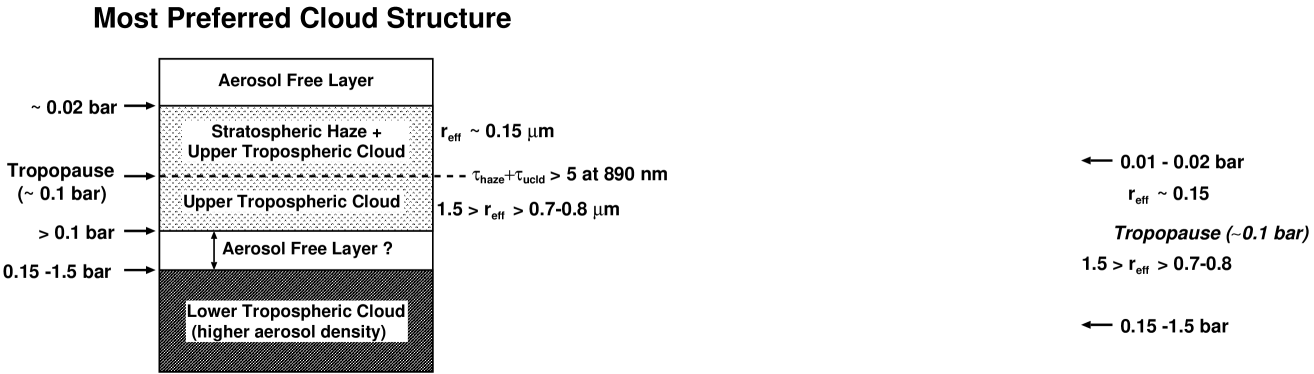
Figure 11: The most favorable model in our modeling analysis of the equatorial region of Saturn.

We discovered that the best-fit modeling parameters depend heavily on assumed cloud structures, choice of aerosol scattering functions and initial optimization conditions. We are presently applying the same fitting method to other latitudes in Saturn’s southern hemisphere and comparing them to discern any latitudinal variation in Saturn’s atmospheric structure. We will also examine the effect of choices of atmospheric composition on the modeling results. These results will be presented in a forthcoming publication.

The Cassini spacecraft will arrive at the Saturnian system in late 2004. It will undoubtedly provide a great deal of new data covering a wide range of phase angle and of very high spatial resolution. Those unique data, which can never be obtained from the earth, will greatly help to examine the Saturn’s aerosol properties and local meteorological phenomena. Nevertheless, ground-based observations with an AOTF camera offer some advantages over the observations by Cassini, such as the extended temporal coverage to track down the seasonal change in Saturn’s atmosphere and the spectral agility that is not obtainable with Cassini’s limited number of fixed narrow-band filters (619-, 727- and 890-nm methane bands and adjacent continuum wavelengths). Therefore, data sets acquired by Cassini and an AOTF camera will be nicely complementary to each other, and the combination of the analysis results from those two different data sets will elucidate Saturn’s cloud structure and its variability over time.

Appendix

A: Photometric Reduction of Saturn Data

The intensity of light from Saturn represents the fraction of incident solar radiation at Saturn that is scattered by its atmosphere. Accordingly, it is convenient to calibrate Saturn’s intensity in terms of the incident solar flux, $\pi F_{\odot}$. We finally obtain the quantity $I/F_{\odot}$, which is a modified ratio of the Saturnian intensity $I$ and the incident solar flux $\pi F_{\odot}$. All the arguments below apply to a certain wavelength ($\lambda$) of interest.

First, we seek the formula for the Saturnian intensity. We focus on a single pixel on the Saturnian image and express the intensity from that pixel as $I$. Then, the total radiation energy, $E$, arriving at Earth per unit time from that pixel is expressed as

$$E=I\cos\theta\cdot dS\cdot d\omega_{E}$$

$$=I\cos\theta\cdot dS\cdot\displaystyle{\frac{S_{E}}{\Delta^{2}}},$$ (6)

where

$\theta$:

The zenith angle of the Earth seen at the considered pixel on Saturn,

$dS$:

The actual area covered by the pixel on Saturn,

$d\omega_{E}$:

The solid angle subtended by the Earth seen from the surface of Saturn,

$S_{E}$:

The cross-section of the Earth when projected in the direction of Saturn,

$\Delta$:

The distance between the Earth and Saturn.

Therefore, the flux $F$ falling on the Earth from that pixel is

$$F=\frac{E}{S_{E}}=I\cdot\frac{cos\theta dS}{\Delta^{2}}.$$ (7)

Note that $\displaystyle{\frac{cos\theta dS}{\Delta^{2}}}$ is the solid angle subtended by the pixel seen from the Earth; we define this as $\omega$. Then,

$$I=\frac{F}{\omega}.$$ (8)

Next, if we define the solar flux incident on Saturn as $\pi F_{\odot,S}$ and that on the Earth as $F_{\odot,E}$ (here, we deliberately define the Solar flux on the Earth as $F_{\odot,E}$, not as $\pi F_{\odot,E}$, for later convenience),

$$\pi F_{\odot,S}=\frac{1}{d_{s}^{2}}\cdot F_{\odot,E}$$ (9)

where $d_{s}$ denotes the heliocentric distance of Saturn.

If we compare the solar flux with the stellar flux of the designated comparison star,

$$m_{star}-m_{\odot}=-2.5\log_{10}\left(\frac{F_{star}}{F_{\odot,E}}\right),$$ (10)

where

$m_{star}$:

Magnitude of the comparison star,

$m_{\odot}$:

Magnitude of the Sun,

$F_{star}$:

Stellar flux,

$F_{\odot,E}$:

Solar flux incident on the Earth.

Therefore,

$$F_{\odot,E}=F_{star}\cdot 10^{0.4(m_{star}-m_{\odot})}.$$ (11)

From (9) and (11), we obtain

$$F_{\odot,S}=\frac{1}{\pi d_{s}^{2}}F_{star}\cdot 10^{0.4(m_{star}-m_{\odot})}$$ (12)

As a consequence of (8) and (12), we obtain the following formula.

$$\frac{I}{F_{\odot,S}}=\frac{\pi d_{s}^{2}}{\omega}\cdot\frac{F}{F_{star}}\cdot 10^{0.4(m_{\odot}-m_{star})}$$

$$=\frac{\pi d_{s}^{2}}{\omega}\cdot 10^{0.4(m_{\odot}-m_{star})}\cdot\frac{F}{F_{star2}}\cdot\frac{F_{star2}}{F_{star}}$$

$$=\frac{\pi d_{s}^{2}}{\omega}\cdot 10^{0.4(m_{\odot}-m_{star})}\cdot\frac{DN}{DN_{star2}}\cdot\frac{DN_{star2}}{DN_{star}}$$ (13)

where,

$DN$:

Observed digital number on the detector obtained at the considered pixel on Saturn image,

$DN_{star}$:

Observed total digital number of the primary standard star on the detector,

$F_{star2}$:

Flux from the secondary standard star,

$DN_{star2}$:

Observed total digital number of the secondary standard star on the detector.

This last equation means that we need only the following information to calibrate Saturnian images : heliocentric distance of Saturn at the time of observation ($d_{s}$), angular pixel scale on the detector ($\omega$), magnitudes of the Sun and the primary standard star ($m_{\odot}$ and $m_{star}$, respectively) and the digital numbers on the detector obtained from the observations of Saturn, primary and secondary standard stars.

B: Calculation of opacity and albedo in an atmospheric layer

In our model, the total opacity ($\tau_{total}$) and effective single-scattering albedo ($\varpi_{0eff}$) of each given atmospheric layer is computed as follows. First, given the pressure levels of layer boundaries, the opacity by Rayleigh scattering gas and its albedo are given as

$$\tau_{R}=\tau_{R,s}+\tau_{R,a}+\tau_{\mbox{\tiny$CH_{4}$}}$$ (14)

and

$$\varpi_{0R}=\displaystyle{\frac{\tau_{R,s}}{\tau_{R}}}$$ (15)

where

$\tau_{R,s}$:

Scattering opacity by Rayleigh gas,

$\tau_{R,a}$:

Absorption opacity by Rayleigh gas in continua,

$\tau_{\mbox{\tiny$CH_{4}$}}$:

Opacity by methane absorption.

Here,

$$\tau_{R,s}=\displaystyle{\frac{\Delta p}{\overline{m}g}\sum_{i}}\alpha_{i}k_{i,s}$$ (16)

$$k_{i,s}=\displaystyle{\frac{32\pi^{3}}{3}\cdot\frac{1}{N^{2}}\cdot\frac{(n_{\lambda,i}-1)^{2}}{\lambda^{4}}\cdot\left(\frac{6+3\delta_{i}}{6-7\delta_{i}}\right)}$$ (17)

$$n_{\lambda,i}-1=A_{i}(1+\displaystyle{\frac{B_{i}}{\lambda[\mu m]^{2}}})$$ (18)

$\alpha_{i}$:

Mixing ratio of i th atmospheric component

$k_{i,s}$:

Scattering coefficient of i th atmospheric component

$\Delta p$:

Pressure difference between top and bottom of the layer

$\overline{m}$:

Mean molecular weight

$g$:

Gravity acceleration

$N$:

Loschmidt number $\equiv$ Number of atoms or molecules in unit volume under the standard temperature and pressure (hereafter, S.T.P. : T=$273.15$[K], P=$1.01325\times 10^{5}$[Pa])

$\delta_{i}$:

Constant to obtain the depolarization factor$\left(\equiv\displaystyle{\frac{6+3\delta_{i}}{6-7\delta_{i}}}\right)$ of i th atmospheric component (Cox 2000)

$n_{\lambda,i}$:

Refractive index of i th atmospheric component at wavelength $\lambda$ under the S.T.P.

$\lambda[\mu m]$:

Wavelength in units of $\mu m$

$A_{i},B_{i}$:

Constants to compute the refractive index of i th atmospheric component at $\lambda[\mu m]$ (Cox 2000)

$\tau_{R,a}$ is obtained when the continuum albedo of Rayleigh gas, $\varpi_{0R,c}$, is given as a free or fixed parameter.

$$\tau_{R,a}=\tau_{R,s}(\displaystyle{\frac{1}{\varpi_{0R,c}}-1})$$ (19)

where,

$$\varpi_{0R,c}\equiv\displaystyle{\frac{\tau_{R,s}}{\tau_{R,s}+\tau_{R,a}}}$$ (20)

In the methane bands, the opacity by methane absorption is calculated as

$$\tau_{\mbox{\tiny$CH_{4}$}}=\displaystyle{\frac{\Delta p}{\overline{m}g}}\alpha_{\mbox{\tiny$CH_{4}$}}k_{\mbox{\tiny$CH_{4}$}}$$ (21)

$\alpha_{\mbox{\tiny$CH_{4}$}}$:

Methane mixing ratio

$k_{\mbox{\tiny$CH_{4}$}}$:

Methane absorption coefficient

In our model, the gravity $g$ is computed from the potential theory that takes into account the ellipticity of the considered planet and the centrifugal force produced by its rotation. Given the planet’s size, mass and ellipticity and rotational period, our code can calculate gravity at any latitude on the planet. For Saturn, we obtained 8.95 $m/s^{2}$ for the equatorial gravity and 12.06 $m/s^{2}$ for the polar gravity.

The aerosol opacity $\tau_{A}$ and aerosol albedo $\varpi_{0A}$ are given as free parameters in aerosol-containing layers.

As a consequence, the total optical thickness and effective single scattering albedo of a layer are generally obtained as :

$$\tau_{total}=\tau_{R}+\tau_{A}$$ (22)

$$\varpi_{0eff}=\displaystyle{\frac{\tau_{R}\cdot\varpi_{0R}+\tau_{A}\cdot\varpi_{0A}}{\tau_{total}}}.$$ (23)

C: Transmission function of the AOTF

The transmission function $T(\nu)$ of the AOTF at the wavenumber $\nu$ $[cm^{-1}]$ is formulated in the following way.

$$T(\nu)=\left(\frac{\sin X}{X}\right)^{2}$$ (24)

where,

$$X\equiv\frac{2.784\cdot(\nu-\nu_{0})}{44.0}$$ (25)

Here, $\nu_{0}$ is the wavenumber in $[cm^{-1}]$ at which the AOTF is tuned to have the maximum transmission. The conversion between $\lambda[nm]$ and $\nu[cm^{-1}]$ simply follows,

$$\nu[cm^{-1}]=\frac{1}{\lambda[nm]\times 10^{-7}}$$ (26)

Acknowledgments

We thank the entire MSSC staff for their help in our observations. In particular, we express our sincere gratitude to Dr. Lewis Roberts for his great assistance in the arrangement of our observations. The US Air Force provided the telescope time, on-site support and 80% of research funds for this AFOSR and NSF jointly sponsored research under grant number NSF AST-0123443. N.J.C. acknowledges support from the Tombaugh Scholars Program.

References

Acarreta, J. R., and A. Sánchez-Lavega 1999. Vertical cloud structure in Saturn’s 1990 equatorial storm. Icarus 137, 24–33.

Atreya, S. K., M. H. Wong, T. C. Owen, P. R. Mahaffy, H. B. Niemann, I. de Pater, P. Drossart, and T. Encrenaz 1999. A comparison of atmospheres of Jupiter and Saturn: deep atmospheric composition, cloud structure, vertical mixing, and origin. Planet. Space. Sci. 47, 1243–1262.

Atreya, S. K., P. R. Mahaffy, H. B. Niemann, M. H. Wong, and T. C. Owen 2003. Composition and origin of the atmosphere of Jupiter - an update, and implications for the extrasolar giant planets. Planet. Space. Sci. 51, 105–112.

Banfield, D., P. J. Gierasch, S. W. Squyres, P. D. Nicholson, B. J. Conrath, and K. Matthews 1996. 2$\mu$m Spectroscopy of Jovian stratospheric aerosols - Scattering opacities, vertical distributions, and wind speeds. Icarus 121, 389–410.

Benassi, M., R. D. M. Garcia, A. H. Karp, and C. E. Siewert 1984. A high-order spherical harmonics solution to the standard problem in radiative transfer. Astrophys. J. 280, 853–864.

Bézard, B., J. P. Baluteau, and A. Marten 1983. Study of the deep cloud structure in the equatorial region of Jupiter from Voyager infrared and visible data. Icarus 54, 434–455.

Bohren, C. F. and D. R. Hoffman 1983. Absorption and Scattering of Light by Small Particles, John Wiley & Sons, New York.

Bevington, P. R, and D. K. Robinson 1992. Data Reduction and Error Analysis for the Physical Sciences, McGraw-Hill, Boston.

Carlson, B. E., A. A. Lacis, and W. B. Rossow 1993. Tropospheric gas composition and cloud structure of the Jovian north equatorial belt. J. Geophys. Res. 98, E3, 5251–5290.

Carlson, B. E., A. A. Lacis, and W. B. Rossow 1994. Belt-zone variations in the Jovian cloud structure. J. Geophys. Res. 99, E7, 14623–14658.

Chandrasekhar, S. 1960. Radiative Transfer, Dover, New York.

Chanover, N. J., C. M. Anderson, C. P. McKay, P. Rannou, D. A. Glenar, J. J. Hillman, and W. E. Blass 2003. Probing Titan’s lower atmosphere with acousto-optic tuning. Icarus 163, 150–163.

Conrath, B. J., D. Gautier, R. A. Hanel, and J. S. Hornstein 1984. The helium abundance of Saturn from Voyager measurements Astrophys. J. 282, 807–815.

Conrath, B. J., and D. Gautier 2000. Saturn helium abundance: A reanalysis of Voyager measurement. Icarus 144, 124–134.

Courtin, R., D. Gautier, A. Marten, B. Bézard, and R. Hanel 1984. The composition of Saturn’s atmosphere at northern temperate latitudes from Voyager IRIS spectra: $NH_{3}$, $PH_{3}$, $C_{2}H_{2}$, $C_{2}H_{6}$, $CH_{3}D$, $CH_{4}$, and the Saturnian D/H isotopic ratio. Astrophys. J. 287, 899–916.

Cox, A. N. 2000. Allen’s Astrophysical Quantities, Springer-Verlag, New York.

Dollfus, A. 1996. Saturn’s rings: Optical reflectance polarimetry. Icarus 124, 237–261.

Dulgach, J. M., A. V. Morozhenko, A. P. Vid’machenko, and E. G. Yanovitskij 1983. Investigations of the optical properties of Saturn’s atmosphere carried out at the main astronomical observatory of the Ukrainian Academy of Sciences. Icarus 54, 319–336.

Esposito, L. W., J. N. Cuzzi, J. B. Holberg, E. A. Marouf, G. L. Tyler, and C. C. Porco 1984. Saturn’s rings: Structure, dynamics and particle properties. In Saturn (T. Gehrels and M. S. Matthews, Eds.) pp. 463–545. University of Arizona Press, Tucson.

Georgiev, G., D.A. Glenar, and J. J. Hillman 2002. Spectral characterization of acousto-optic filters used in imaging spectroscopy. Appl. Optics 41, 209–217.

Glenar, D. A., J. J. Hillman, B. Saif, and J. Bergstralh 1994. Acousto-optic imaging spectropolarimetry for remote sensing. Appl. Optics 33, No.31, 7412–7424.

Glenar, D.A., J. J. Hillman, M. Lelouarn, R. Q. Fugate, and J. D. Drummond 1997. Multispectral imagery of Jupiter and Saturn using adaptive optics and acousto-optic tuning. Publ. Astron. Soc. Pac. 109, 326–337.

Hanel, R., B. Conrath, F. M. Flasar, V. Kunde, W. Maguire, J. Pearl, J. Pirraglia, R. Samuleson, L. Herath, M. Allison, D. Cruikshank, D. Gautier, P. Gierasch, L. Horn, R. Koppany, and C. Ponnamperuma 1981. Infrared observations of the Saturnian system from Voyager 1. Science 212, 192–200.

Hansen, J. E. 1969. Radiative transfer by doubling very thin layers. Astrophys. J. 155, 565–573.

Hansen, J.E. and L.D.Travis 1974. Light scattering in planetary atmospheres. Space Sci. Rev. 16, 527–610.

Hardorp, J. 1980. The Sun among the stars III. Energy distributions of 16 northern G-type stars and the solar flux calibration. Astron. Astrophys. 91, 221–232.

Karkoschka, E. and M. G. Tomasko 1992. Saturn’s upper troposphere 1986–1989. Icarus 97, 161–181.

Karkoschka, E. and M. G. Tomasko 1993. Saturn’s upper atmospheric hazes observed by the Hubble Space Telescope. Icarus 106, 428–441.

Karkoschka, E. 1994. Spectrophotometry of the Jovian planets and Titan at 300- to 1000-nm wavelength: The methane spectrum. Icarus 111, 174–192.

Lindal, G. F., D. N. Sweetnam, and V. R. Eshleman 1985. The atmosphere of Saturn: An analysis of the Voyager radio occultation measurements. Astron. J. 90, 1136–1146.

Marten, A., D. Rouan, J. P. Baluteau, D. Gautier, B. J. Conrath, R. A. Hanel, V. Kunde, R. Samuelson, A. Chedin, and N. Scott 1981. Study of the ammonia ice cloud layer in the equatorial region of Jupiter from the infrared interferometric experiment on Voyager. Icarus 46, 233–248.

O’Brien, J.J., and H. Cao 2002. Absorption spectra and absorption coefficients for methane in the 750–940 nm region obtained by intracavity laser spectroscopy. J. Quant. Spectrosc. Radiat. Transf. 75, 323–350.

Ortiz, J. L., F. Moreno, and A. Molina 1995. Saturn 1991-1993: Reflectivities and limb-darkening coefficients at methane band and nearby continua – Temporal changes. Icarus 117, 328–344.

Ortiz, J. L., F. Moreno, and A. Molina 1996. Saturn 1991-1993: Clouds and hazes. Icarus 119, 53–66.

Potter, J. F. 1970. The delta function approximation in radiative transfer theory. J. Atmos. Sci. 27, 943–949.

Sanchez-Lavega, A., J. Lecacheux, F. Colas, and P. Laques 1994. Photometry of Saturn’s 1990 equatorial disturbance Icarus 108, 158–168.

Santer, R., and A. Dollfus 1981. Optical reflectance polarimetry of Saturn’s globe and rings : IV. Aerosol in the upper atmosphere of Saturn. Icarus 48, 496–518.

Singh, K., and J. J. O’Brien 1995. Laboratory measurements of absorption coefficients for the 727 nm band of methane at 77 K and comparison with results derived from spectra of the giant planets. J. Quant. Spectrosc. Radiat. Transf. 54, 607–619.

Sromovsky, L. A., and P. M. Fry 2002. Jupiter’s cloud structure as constrained by Galileo probe and HST observations. Icarus 157, 373–400.

Stam, D. M., D. Banfield, P. J. Gierasch, P. D. Nicholson, and K. Matthews. 2001. Near-IR spectrophotometry of Saturnian aerosols – meridional and vertical distribution. Icarus 152, 407–422.

Stammes, P., J. F. de Haan, and J. W. Hovenier 1989. The polarized internal radiation field of a planetary atmosphere. Astron. Astrophys. 225, 239–259.

Stamnes, K., S. C. Tsay, W. Wiscombe, and K. Jayaweera 1988. Numerically stable algorithm for discrete-ordinate-method radiative transfer in multiple scattering and emitting layered media. Appl. Optics 27, 2502–2509.

Thomas, G.E., and K. Stamnes 1999. Radiative Transfer in the Atmosphere and Ocean, Cambridge University Press, Cambridge, U.K.

Tomasko, M.G., R. S. McMillan, L. R. Doose, N. D. Castillo, J. P. Dilley 1980. Photometry of Saturn at large phase angles. J. Geophys. Res. 85, A11, 5891–5903.

Tomasko, M.G. and L. R. Doose 1984. Polarimetry and Photometry of Saturn from Pioneer 11 : Observations and constraints on the distribution and properties of cloud and aerosol particles. Icarus 58, 1–34.

Weidenschilling, S. J., and J. S. Lewis 1973. Atmospheric and cloud structures of the Jovian planets. Icarus 20, 465–476.

West, R. A., M. G. Tomasko, B. A. Smith, M. P. Wijesinghe, L. R. Doose, H. J. Reitsema, and S. M. Larson 1982. Spatially resolved methane band photometry of Saturn I, Absolute reflectivity and center-limb variations in the 6190-, 7250-, and 8900-Åbands. Icarus 51, 51–64.

West, R.A. 1983. Spatially resolved methane band photometry of Saturn II, Cloud structure models at four latitudes. Icarus 53, 301–309.

West, R.A., M. Sato, A. L. Hart, C. W. Hord, K. E. Simmons, L. W. Esposito, D. L. Coffeen, R. B. Pomphrey 1983. Photometry and polarimetry of Saturn at 2640 and 7500 Å. J. Geophys. Res. 88, A11, 8679–8697.