Using Fractal Dimensionality in the Search for Source Models of Ultra-High Energy Cosmic Rays

Abstract

Although the existence of cosmic rays with energies extending well above $10^{19}$ eV has been confirmed, their origin remains one of the most important questions in astro-particle physics today. Several source models have been proposed for the observed set of Ultra High Energy Cosmic Rays (UHECRs). Yet none of these models have been conclusively identified as corresponding with all of the available data. One possible way of achieving a global test of anisotropy is through the measurement of the information dimension, $D_{\rm I}$, of the arrival directions of a sample of events. $D_{\rm I}$ is a measure of the intrinsic heterogeneity of a data sample. We will show how this method can be used to take into account the extreme asymmetric angular resolution and the highly irregular aperture of a monocular air-fluorescence detector. We will then use a simulated, isotropic event sample to show how this method can be used to place upper limits on any number of source models with no statistical penalty.

1 Introduction

The observation of Ultra High Energy Cosmic Rays (UHECRs) has now spanned nearly three decades. Over that period, many different source models have been proposed to explain the origin of these remarkable events. Recently, the Akeno Giant Air Shower Array (AGASA) reported clustering at small angular scales for the events that were observed above $4\times 10^{19}$ eV [1]. However, this result could not be confirmed by the High Resolution Fly’s Eye (HiRes) air fluorescence detector [2] despite the fact that Hires-I’s monocular exposure was more than twice that of AGASA within the pertinent energy range [3]. AGASA has also reported a possible excess of events in the direction of the galactic center for events with energies around $10^{18}$ eV [4]. However, HiRes reported that it did not see anisotropies when examining harmonics in right ascension, a priori determined point sources, or enhancement in the supergalactic plane. Furthermore, prior analysis by the the original Fly’s Eye showed no evidence of anisotropies when dependencies in galactic latitude and longitude, harmonics in right ascension, excess maps, and specific a priori determined point sources were examined [5, 6]. However, Fly’s Eye did find a small apparent excess in the direction of the galactic plane. [7]. In 1995, it was reported by Stanev et al. that the combined data of Haverah Park, Yakutsk, and AGASA showed an excess along the supergalactic plane with several potential point sources for events above $2\times 10^{19}$ eV [8].

These conflicting reports call for developing a more global way in which one could determine if a given sample possesses any statistically significant anisotropy. We will show that by considering the information dimension, $D_{\rm I}$, of a given sample, one can simultaneously look for anisotropies at all angular scales greater than the angular resolution of the sample by considering the intrinsic heterogeneity of that particular data sample. This method is quite robust in that it can easily accommodate both asymmetric angular resolutions and irregular apertures. Furthermore, in the event that a sample is shown to be consistent with an isotropic distribution, this method can be used to place upper limits on possible source models. Because only a single measurement is taken of the actual data, any number of source models can be considered simultaneously without incurring statistical penalties.

2 Calculating Fractal Dimensions of a Data Sample

Fractal dimensionality is a simple measure of the scaling symmetry of a structure. By measuring the fractal dimension of a data sample, one can examine its self-consistency at different levels of magnification. There are several ways of exploiting this idea. From a computational perspective, the simplest is to use box-counting. For the most general case, the capacity dimension, $D_{\rm c}$ [9], one partitions the sample space into equi-sized and equi-shaped “boxes” with edge size $\epsilon$:

$$D_{\rm c}=\lim_{\epsilon\to 0^{+}}\frac{\log{\it N}(\epsilon)}{\log 1/\epsilon}.$$ (1)

Here, $N(\epsilon)$ is the minimum number of “boxes” with edge size $\epsilon$ necessary to cover one’s sample.

The capacity dimension has a serious limitation: It only looks for the presence of the sample within the available space and does not consider variations in the density of the sample at a given point in space. In cases where the density may differ within the sample space, the appropriate alternative is to use the information dimension, $D_{\rm I}$ [10, 11]:

$$D_{\rm I}=-\sum_{i=1}^{N}\lim_{\epsilon\to 0^{+}}\frac{P_{\rm i}(\epsilon)\log P_{\rm i}(\epsilon)}{\log 1/\epsilon},$$ (2)

where $P_{\rm i}(\epsilon)$ is the probability of finding a data point in the $i$-th box of edge size $\epsilon$. This is a particularly suitable measurement when considering a data set consisting of UHECR arrival directions with finite angular resolution.

It should be noted that $D_{\rm C}$ and $D_{\rm I}$ are both particular cases of the $q$-dimension [12, 13],

$$D_{q}=\frac{1}{1-q}\lim_{\epsilon\to 0^{+}}\frac{\log I(q,\epsilon)}{\log 1/\epsilon};$$ (3)

where

$$I(q,\epsilon)=\sum_{i=1}^{N}P_{\rm i}(\epsilon)^{q}.$$ (4)

We can then see that $D_{\rm C}=\lim_{q\to 0}D_{q}$ and that $D_{\rm I}=\lim_{q\to 1}D_{q}$.

3 Application to Arrival Direction Distributions for UHECRs

In principle, it is simple to calculate the information dimension for a given sample of events. However, two complications arise when considering a set of arrival directions of UHECRs. First, the event directions are not known with complete precision. This makes the determination of $D_{\rm I}$ as $\epsilon\to 0$ meaningless. Secondly, the determination of $D_{\rm I}$ requires that the sample space be divided into equi-sized and equi-shaped bins. For a spherical surface, this is simply not possible. Nevertheless, there are workable solutions for both of these problems.

3.1 Angular Resolution

We will consider a hypothetical monocular air-fluorescence detector. This detector is largely based upon the characteristics of the Hires-I detector [14, 15]. Our detector observes events with an angular resolution that is described by a highly asymmetric 2-d Gaussian.

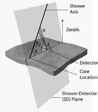
Figure 1: The geometry of reconstruction for a monocular air fluorescence detector

For a monocular air fluorescence detector, angular resolution consists of two components: $\sigma_{\rm 1}$, in the determination of the angle, $\psi$, within the plane of reconstruction, and $\sigma_{\rm 2}$, in the estimation of the plane of reconstruction itself. Figure 1 illustrates how this geometry would appear with a particular plane of reconstruction and a particular value for $\psi$. Intuitively, we can see that we should be able to determine the plane of reconstruction quite accurately. However, the value of $\psi$ is more difficult to determine because it is dependent on the precise results of the monocular reconstruction [14, 15].

The actual parameterizations of $\sigma_{\rm 1}$ and $\sigma_{\rm 2}$ assumed are as follows:

$$\sigma_{\rm 1}=20^{\circ}e^{-1.5\log_{\rm 10}E_{\rm EeV}}+4^{\circ}$$ (5)

and

$$\sigma_{\rm 2}=100^{\circ}e^{-0.5\Delta\chi}+0.4^{\circ}.$$ (6)

Here, $E_{\rm EeV}$ is the primary energy of the shower in EeV. For the purpose of this study, the energy will be allowed to vary between $10^{18.5}$ eV and $10^{20}$ eV with a differential spectral index of $-2.7$. In this scenario, a shower with a primary energy of $10^{18.5}$ eV will have $\sigma_{\rm 1}=13.4^{\circ}$, while a shower with a primary energy of $10^{20}$ eV will have $\sigma_{\rm 1}=5.0^{\circ}$. This difference can be attributed to the fact that larger showers have better defined profiles and a better signal-to-noise ratio.

The factor, $\Delta\chi$, in equation 6 is the angular track length (in degrees) of the shower as observed by the detector, which is allowed to vary between $8^{\circ}$ and $30^{\circ}$. A shower with an observed track length of $8^{\circ}$ will have $\sigma_{\rm 2}=2.2^{\circ}$, while a shower with an observed track length of $30^{\circ}$ will have $\sigma_{\rm 2}=0.4^{\circ}$; a longer track-length leads to a more accurate determination of the plane of reconstruction. The distribution of $\sigma_{\rm 2}$ values is largely independent of energy because while higher energy showers do lead to more longitudinal development, they are also brighter, which allows one to observe them at greater distances. These competing factors lead to $\Delta\chi$ distributions that are virtually identical across the observed spectrum.

In general, it should be noted the distributions of $\sigma_{\rm 1}$ and $\sigma_{\rm 2}$ values are relatively insensitive to the differential spectral index that is chosen. We ascertained this by considering two sets, one with a differential spectral index of $-2.5$ and one with a differential spectral index of $-3.5$. Even for a variation that was much larger than the accepted range of experimental values for the the UHECR spectrum [14, 15, 16, 17], the value of $\bar{\sigma_{\rm 1}}$ increased by only $11\%$. The value of $\bar{\sigma_{\rm 2}}$ remained unchanged. This can be explained by realizing for a steeply falling spectrum, the overwhelming majority of observed events in either case will occur in the first half decade of the measurement. This is a very small effect compared to the expected statistical fluctuations that would occur between two consecutive sets of observations.

For the purpose of calculating $D_{\rm I}$, we can treat the arrival direction of each individual shower as a two dimensional elliptical Gaussian distribution with the parameters $\sigma_{\rm 1},\sigma_{\rm 2}$. The size of a bin’s edge, $\epsilon$, will be allowed to take on a series of values, $\Delta\theta$, which will be in an interval corresponding to a scale length of the sample or in the case of a smooth distribution, the smallest value that is computationally feasible. For finite events samples, we will use $\Delta\theta\simeq 0.5^{\circ}$. In the case of smooth distributions we will use a computationally limited value of $\Delta\theta=1/6^{\circ}$. The number of points in each shower direction distribution, $N_{\rm Dist}$, will be determined by the mean value, $<\!\!n_{\rm i}\!\!>$, necessary to assure that the fractional Gaussian fluctuations of the count, $n_{\rm i}$, in each bin, do not on average, exceed a predetermined value (i.e. for $5\%$ fluctuations, $N_{\rm Dist}\simeq 500$). For each value of $\epsilon$, the probability, $P_{\rm i}(\epsilon)$, for the $i$-th bin will be:

$$P_{\rm i}(\epsilon)=\frac{n_{\rm i}}{N_{\rm Dist}\cdot N_{\rm Shower}}.$$ (7)

We calculate $D_{\rm I}$ for each value of $\epsilon$:

$$D_{\rm I}(\epsilon)=-\sum_{i=1}^{N}\frac{P_{\rm i}(\epsilon)\log P_{\rm i}(\epsilon)}{\log 1/\epsilon}.$$ (8)

We then determine $D_{\rm I}$ to be $<\!\!D_{\rm I}(\epsilon)\!\!>$ over the specified interval of $\epsilon$ values.

3.2 Latitudinal Binning

For the purpose of calculating $D_{\rm I}$, it is necessary that all bins be equi-sized and equi-shaped as we vary the size of the side of the bins, $\epsilon$. While it is impossible to achieve completely this criterion on the surface of a sphere, we will be able to do so approximately by adopting a latitudinal binning scheme.

Latitudinal binning is achieved by first dividing the sky into $N_{\rm\delta}$ declinational $(\delta)$ bands where each band has a width

$$\Delta\theta=\frac{\pi}{N_{\rm\delta}}$$ (9)

For each declinational band, the sky is then divided into $N_{\rm\alpha,\delta}$ bins in right ascension $(\alpha)$ where:

$$N_{\rm\alpha,\delta}=\biggr{[}\frac{2\pi\int_{\delta 1}^{\delta 2}\cos\delta\,d\delta}{(\Delta\theta)^{2}}\biggr{]}=\biggr{[}\frac{2(N_{\rm\delta})^{2}\int_{\delta 1}^{\delta 2}\cos\delta\,d\delta}{\pi}\biggr{]}.$$ (10)

The solid angle, $\Delta\Omega_{\rm\delta}$ of each bin (in steradians) is:

$$\Delta\Omega_{\rm\delta}=\frac{2\pi\int_{\delta 1}^{\delta 2}\cos\delta\,d\delta}{N_{\rm\alpha,\delta}},$$ (11)

with a minimum value of $(\Delta\theta)^{2}$ (at the equator) and a maximum value of $\frac{\pi}{3}(\Delta\theta)^{2}$ (at the poles) regardless of the value of $N_{\rm\delta}$. This provides us with bins that are all almost the same area and nearly square-shaped (with the exception of three triangular bins at each pole). The total number of bins in the sky can be approximated by:

$$N_{sky}\simeq 4\pi(\frac{N_{\rm\delta}}{\pi})^{2}=\frac{4}{\pi}(N_{\rm\delta})^{2}.$$ (12)

In figure 2, we visualize the latitudinal binning technique for a series of different $N_{\rm\delta}$ values.

(a)	(b)
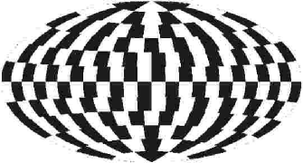
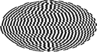
(c)	(d)

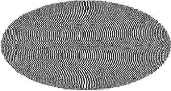
Figure 2: Hammer-Aitoff projection of latitudinal bins for four different values of $N_{\rm\delta}$—(a): $N_{\rm\delta}=5$; (b): $N_{\rm\delta}=12$; (c): $N_{\rm\delta}=30$; (d): $N_{\rm\delta}=90$.

3.3 Application to the Calculation of $D_{\rm I}$

We can now apply the preceding machinery to the calculation of $D_{\rm I}$: First, we need to normalize the event count in each bin by its respective bin area, $\Delta\Omega_{\rm\delta}$:

$$P_{\rm i}(\epsilon)=\frac{n_{\rm i}(\Delta\theta)^{2}}{N_{\rm Dist}N_{\rm Shower}\Delta\Omega_{\rm\delta}}=\frac{n_{\rm i}\pi^{2}}{N_{\rm Dist}N_{\rm Shower}(N_{\rm\delta})^{2}\Delta\Omega_{\rm\delta}}.$$ (13)

If we then realize that $\epsilon=\frac{1}{N_{\rm\delta}}$, we can obtain:

$$D_{\rm I}(N_{\rm\delta})=-\frac{1}{\log N_{\rm\delta}}\sum_{i=1}^{N}P_{\rm i}(N_{\rm\delta})\log P_{\rm i}(N_{\rm\delta}).$$ (14)

This expression is reminiscent of the the general formula for entropy from statistical mechanics:

$$S=-k\sum_{r}p_{r}\log p_{r};$$ (15)

where $p_{r}$ is the probability of a particle being the $r$-th state and $k$ is the Boltzmann constant, which can be thought of as a scaling constant based upon the intrinsic scale of the given particle. The information dimension, $D_{\rm I}$, is an analogous measurement of the heterogeneity of a given data set.

4 Calculating $D_{\rm I}$ for Exposures of Different Source Models

4.1 Exposure-Independent Source Descriptions

We began by examining four different source models independently of detector exposure. This allows us to calculate the value of the information dimension, $D_{\rm I}$, without consideration to the detector aperture or statistical fluctuations from a finite event sample. The source models are: an isotropic source model, a dipole source model, a model with seven sources superimposed on an isotropic background, and a dark matter halo source model.

4.1.1 Isotropic Model

The first model that we will consider is an isotropic source model with distribution:

$$n_{\rm isotropic}=1.$$ (16)

4.1.2 Dipole Model

The second is the Centaurus A dipole source model first proposed by Farrar and Piran [18]. This model has a distribution of arrival directions characterized by a scaling parameter, $\alpha$, which can take on any value between $-1$ and $+1$ and by $\theta$, which is the opening angle between a given event arrival direction and the center of the dipole distribution at Centaurus A. The overall distribution is:

$$n_{\rm dipole}=1+\alpha\cos\theta.$$ (17)

4.1.3 Discrete Source Model

The third model that we will consider is one with seven discrete sources superimposed on an isotropic background. For simplicity’s sake, we will assume that all seven sources have an equal intensity indirectly determined by a parameter, $F_{s}$, which will be defined as the fraction of the entire event sample which originates in the seven sources. We will define our source direction to be the centroids of the seven hypothetical point sources proposed by the AGASA collaboration [1]. The equatorial coordinates used for each point source are listed in table 1

Cluster	Right Ascension	Declination
C1	01h13m	$20.6^{\circ}$
C2	11h17m	$56.9^{\circ}$
C3	18h51m	$48.2^{\circ}$
C4	04h38m	$30.0^{\circ}$
C5	16h02m	$23.3^{\circ}$
C6	14h11m	$37.4^{\circ}$
C7	03h03m	$55.5^{\circ}$

Table 1: Coordinates used for the centers of seven discrete sources. These coordinates correspond to the centers of the seven clusters reported by the AGASA Collaboration [1].

The arrival directions for the events from each source are assumed to be subjected to magnetic smearing. That is, in the course of traveling through space from the source to the point of observation, the velocity vector of the event is subject to bending in the galactic and extra-galactic magnetic fields. We assumed that this bending produces an apparent source that can be characterized by a Gaussian distribution:

$$P(\Delta\theta)=\frac{\Delta\theta}{\lambda^{2}}e^{-\frac{(\Delta\theta)^{2}}{2\lambda^{2}}},$$ (18)

where $P(\Delta\theta)$ is the probability that an event will be observed with an opening angle, $\Delta\theta$, from the nominal direction of the apparent source. We will also assume that the arrival directions of the events from all the sources are subject to the same degree of magnetic smearing, parameterized by $\lambda_{\circ}=1.5105\cdot\lambda$. The parameter, $\lambda_{\circ}$, corresponds to the 68% confindence interval in $\Delta\theta$. For this paper, we will assume that $\lambda_{\circ}=5^{\circ}$. It should be noted that the nominal direction of the apparent source is not necessarily the direction of the actual source because the possibility exists that the path of the events in question traveled through large regions of homogeneous magnetic fields.

4.1.4 Dark Matter Halo Model

The fourth model that we will consider is a dark matter halo source model. Dark matter halos are characterized by a density profile that is assumed to take the Navarro-Frenk-White (NFW) form [19]:

$$\rho_{\rm NFW}=\frac{\rho_{\circ}}{r(1+r/r_{\rm s})^{2}},$$ (19)

where $\rho_{\circ}$ is a dark matter density parameter, $r$ is the distance from the center of the halo, and $r_{\rm s}$ is a critical radius. For our source model, we will consider the contribution of only the four closest significant dark matter halos: the Milky Way, M31, LMC, and M33. We will assume that $\rho_{\circ}$ is the same for all four sources and that $r_{\rm s}$ scales with the cube root of the luminosity, $L^{\frac{1}{3}}$. Thus the Milky Way will have: $r_{\rm s,MW}=10.0$ kpc, LMC will have $r_{\rm s,LMC}=0.3\cdot r_{\rm s,MW}=3.0$ kpc, M31 will have $r_{\rm s,M31}=1.5\cdot r_{\rm s,MW}=15.0$ kpc, and M33 will have $r_{\rm s,M33}=0.4\cdot r_{\rm s,MW}=4.0$ kpc.

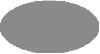
(a)	(b)
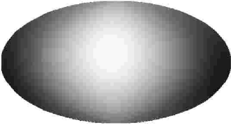
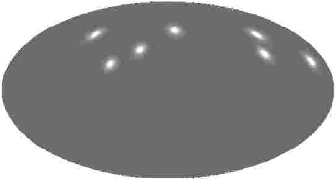
(c)	(d)

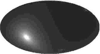
Figure 3: Density profiles for four different source models—(a): isotropic model; (b): dipole enhancement model $(\alpha=1.0)$; (c): seven source model $(F_{s}=0.28)$; (d): dark matter halo model $(r_{s}=10~{}{\rm kpc})$. All four figures are shown in a Hammer-Aitoff projection of equatorial coordinates (right ascension right to left). The highest density in each panel corresponds to the lightest (red) regions, the lowest density to the darkest (blue) regions.

We now calculate the information dimension, $D_{\rm I}$, for each of the our four models. Since these are smooth distributions with no statistical fluctuations, we will only use one, computationally limited value for the number of declinational bands for each model of $N_{\rm\delta}=1080$ (i.e. $\Delta\theta=\frac{1}{6}^{\circ}$), which implies:

$$P_{\rm i}=n_{\rm i}\biggr{[}\sum_{\rm i}n_{\rm i}\biggr{]}^{-1}.$$ (20)

Using equations 14 and 20 we can now calculate $D_{\rm I}$ for each of the four models. The results are in table 2 column 1. Note that three of the four values of $D_{\rm I}$ exceed the analytical limit of $2$ for a 2-D surface.

If we consider the analytic limit for the isotropic case, we have:

$$D_{\rm I}=-4\frac{(N_{\rm\delta})^{\rm 2}}{\pi}\frac{P_{\rm i}\log P_{\rm i}}{\log N_{\rm\delta}}.$$ (21)

If we then substitute in equation 20 we get:

$$D_{\rm I}=\frac{2\log N_{\rm\delta}+\log 4/\pi}{\log N_{\rm\delta}};\lim_{N_{\rm\delta}\to\infty}D_{\rm I}(N_{\rm\delta})=2.$$ (22)

The reason the we obtain values greater than $2$ is because we are working with a finite number of elements on a surface where the total area does not equal $(N_{\rm\delta})^{2}$.

Intrinsic $D_{\rm I}$ values for the different source models that we examined in figures 3 and 5.

	1	2
	$D_{\rm I}$ for Source Model	$D_{\rm I}$ for Source Model
SOURCE MODEL	without	with
	Detector Exposure	Detector Exposure
Isotropic	2.035	1.967
Dipole Enhancement	2.007	1.945
Seven Source	2.033	1.946
Dark Matter Halo Model	1.999	1.978

Table 2: The estimated values of $D_{\rm I}$ with $N_{\rm\delta}=1800$ for the four proposed source models for the entire sky independent of any real detector’s aperture (1) and for the four source models superimposed on the estimated aperture of an air-fluorescence detector at $40^{\circ}~{}N$. These values are mathematical descriptors of a data set that are whose number of significant digits are determined by how extensively each bin is sampled (in this case four digits). In the case of a real data set with a finite number of the observations, the number of significant digits is constrained by the fluctuations inherent to the sample size

4.2 Exposure-Dependent Source Descriptions

For the purpose of this paper, we assume a hypothetical air-fluorescence detector located at $40^{\circ}~{}N$. This analysis assumes an isotropic distribution for the azimuthal component of the arrival directions and a zenith angle distribution that remains constant in time. This is what one would expect for a detector with $360^{\circ}$ coverage with identical detector units and stable atmospheric conditions. The acceptance of our detector can thus be defined by two distributions: zenith angle and sidereal time which are shown in figure 4. The zenith angle distribution is characterized by $100\%$ acceptance until $\sim 50^{\circ}$, at which point it drops off dramatically due to the lack of a well-defined profile to assist monocular reconstruction. The sidereal time distribution is the combination of the seasonal availability of dark, moonless sky at $40^{\circ}~{}N$ and seasonal climatic changes in a desert locale (the rainy season is assumed to extend from February to May which results in a loss of $\sim 30\%$ of exposure).

By defining acceptance this way, we can calculate the exposure of the detector. By also considering the finite, asymmetric angular resolution, we can then superimpose the detector exposure upon the various source models that we previously examined (figure 3 and table 2 column 1). We then obtain an effective detector response for the air fluorescence detector for each of our four source models. The results are shown in figure 5. It should be emphasized that effective detector effect is due to the combined effect of asymmetric sky coverage and angular resolution smearing. A remarkable consequence of this combination is the possibility that point sources can take on an apparently asymmetric shapes due to preferential orientations of the plane of reconstruction for events arriving from a specific location in the physical sky.

(a)

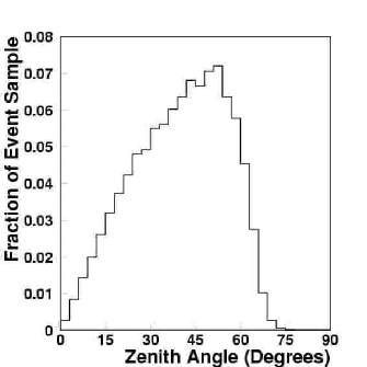
(b)

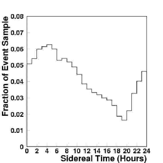
Figure 4: (a): The distribution of zenith angles for a monocular air-fluorescence detector; (b): the distribution sidereal times for a air-fluorescence detector located at $40^{\circ}~{}N$ in a desert locale (right)

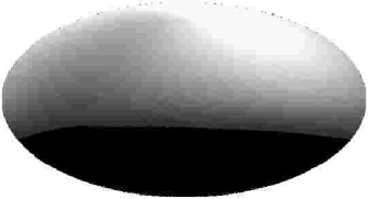
(a)	(b)
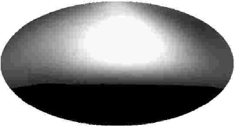
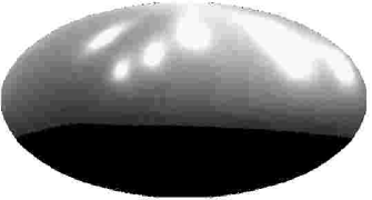
(c)	(d)

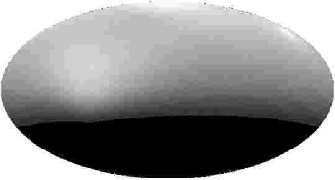
Figure 5: Effective detector response for the four different source models—(a): isotropic model; (b): dipole enhancement model $(\alpha=1.0)$; (c): seven source model $(F_{s}=0.28)$; (d): dark matter halo model $(r_{s}=10~{}{\rm kpc})$. All four figures are shown in a Hammer-Aitoff projection of equatorial coordinates (right ascension right to left). The highest density in each panel corresponds to the lightest (red) regions, the lowest density to the darkest (blue) regions.

We can now determine the value of $D_{\rm I}$ using the same method as before. The results are shown in table 2 column 2. It is interesting to note that the dark matter halo source model now has a larger value for $D_{\rm I}$ than the isotropic source model. By looking at figure 5, one can verify that the superposition of the detector exposure and source models actually yields a more uniform apparent distribution for the dark matter halo source model than it does for the isotropic source model.

5 Calculating $D_{\rm I}$ for Finite Event Samples

So far, we have only considered calculating $D_{\rm I}$ for smooth distributions. From an experimental standpoint, it is very difficult to collect enough data to obtain a smooth distribution. This is especially true for UHECRs. In order to make a measurement of $D_{\rm I}$, we must first determine what value(s) we should assign to $N_{\rm\delta}$. A reasonable approach is to assign a scale length to our sample. Choosing $\Delta\theta=0.5^{\circ}$, which approximately reflects the lowest value that can be obtained from $\sigma_{\rm 2}$ in equation 6, yields $N_{\rm\delta}=360$.

However, it can be beneficial to actually calculate $D_{\rm I}$ for a range of values around $N_{\rm\delta}$. In figure 6a,

(a)

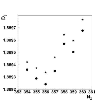
(b)

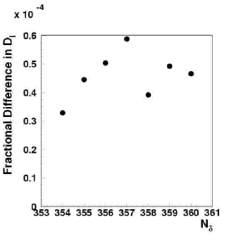
Figure 6: (a): $D_{\rm I}$ over a range of values of $N_{\rm\delta}$ for two similar finite event sets that have similar values for $D_{\rm I}$. (the dots indicate the values $D_{\rm I}$ for the first set while the stars indicate the values $D_{\rm I}$ for the second set); (b): the fractional difference in $D_{\rm I}$ for the same two sets over the range of $N_{\rm\delta}$ values.

we display the values $D_{\rm I}(N_{\rm\delta})$ over the range $N_{\rm\delta}=[354,360]$ for two separate simulated sets where $N_{\rm Shower}=500$. These sets yield very similar values for $D_{\rm I}$ over the full range of values for $N_{\rm\delta}$. However, if we examine figure 6b we can see that for the same two finite samples, the fractional difference between values of $D_{\rm I}$ can fluctuate substantially even over small intervals of $N_{\rm\delta}$. While these fluctuations are typically much smaller than the difference in $D_{\rm I}$ values between any two sets, we will take $D_{\rm I}$ to be $<\!\!D_{\rm I}(N_{\rm\delta})\!\!>$ for the interval: $N_{\rm\delta}=[354,360]$ in order to minimize the statistical fluctuations in $D_{\rm I}$ between individual sets. This range was chosen to optimize our computational ability.

To account for the fact that we no longer have a smooth distribution for the calculation of the values of $P_{\rm i}$, we refer back to equation 13 to see how to calculate $D_{\rm I}$ for a finite set of elements. This only requires us to determine a value for $N_{\rm Dist}$. We can set this value based upon what value we wish for $n_{\rm i}$ in combination with equation 12 (i.e. $<\!\!n_{\rm i}\!\!>=\frac{1}{(\Delta n)^{2}}$ where $\Delta n$ is the fractional Gaussian fluctuation of a bin with $n_{\rm i}=<\!\!n_{\rm i}\!\!>$). Then,

$$N_{\rm Dist}=\frac{\frac{4}{\pi}(N_{\rm\delta})^{2}<\!\!n_{\rm i}\!\!>}{N_{\rm Shower}}.$$ (23)

If we then combine equations 9, 13, and 23; we obtain:

$$P_{\rm i}(N_{\rm\delta})=\frac{n_{\rm i}}{<\!\!n_{\rm i}\!\!>}\frac{\pi^{3}}{4(N_{\rm\delta})^{4}\Delta\Omega_{\rm\delta}}.$$ (24)

We can then calculate $D_{\rm I}$ from equation 14:

$$D_{\rm I}=\biggr{<}\!\!-\frac{1}{\log N_{\rm\delta}}\sum_{i=1}^{N}P_{\rm i}(N_{\rm\delta})\log P_{\rm i}(N_{\rm\delta})\!\biggr{>},\>N_{\rm\delta}=[354,360].$$ (25)

Thus, If we want $<\!\!n_{\rm i}\!\!>=500$ and $N_{\rm Shower}=500$, we find that $N_{\rm Dist}\simeq 1.65\times 10^{5}$. If $N_{\rm Shower}=2000$, we have $N_{\rm Dist}\simeq 4.1\times 10^{4}$.

We now consider two cases: finite event sets with 500 events and finite event sets with 2000 events. These sets will have the angular resolution characteristics described in equations 5 and 6. The exposure will be modeled via the zenith angle and sidereal time distributions shown in figure 4. Figure 7 contains examples of event sets with all four source models and $N_{\rm Shower}=500$ and figure 8 contains examples of events sets with all four previously described source models and $N_{\rm Shower}=2000$.

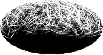
(a)	(b)
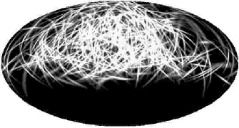
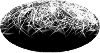
(c)	(d)

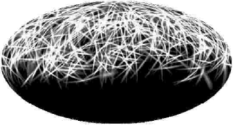
Figure 7: Simulated 500 event distributions for four different source models — (a): Isotropic model; (b): dipole enhancement model $(\alpha=1.0)$; (c): seven source model $(F_{s}=0.28)$; (d): dark matter halo model $(r_{s}=10~{}{\rm kpc})$. All four figures are shown in a Hammer-Aitoff projection of equatorial coordinates (right ascension right to left). The highest density in each panel corresponds to the lightest (red) regions, the lowest density to the darkest (blue) regions.

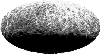
(a)	(b)
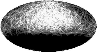
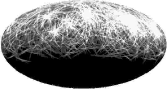
(c)	(d)

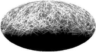
Figure 8: Simulated 2000 event distributions for four different source models — (a): Isotropic model; (b): dipole enhancement model $(\alpha=1.0)$; (c): seven source model $(F_{s}=0.28)$; (d): dark matter halo model $(r_{s}=10~{}{\rm kpc})$. All four figures are shown in a Hammer-Aitoff projection of equatorial coordinates (right ascension right to left). The highest density in each panel corresponds to the lightest (red) regions, the lowest density to the darkest (blue) regions.

In figures 7 and 8 one can see the that these distributions of arrival directions have a far greater degree of statistical fluctuation than the smooth distributions shown in figure 5. Because of the fluctuations in our simulated event samples, the value of $D_{\rm I}$ varies significantly (see figures 9 and 10) from one simulated set to the next. In figures 9 and 10, we examine the distribution of $D_{\rm I}$ values for $\sim 500$ sets (of 500 and 2000 events respectively). We see that the distribution of 500 event samples have both a lower mean value and larger width than the 2000 event samples.

(a)

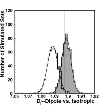
(b)

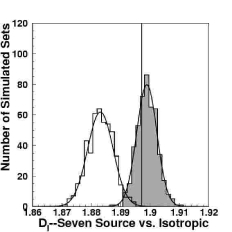
(c)

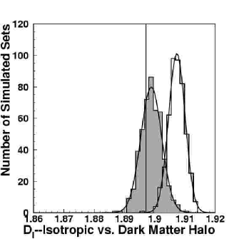
Figure 9: Comparison of distributions of $D_{\rm I}$ values for $\sim 500$ sets of 500 events between the isotopic source model (shaded) and the other three source models — (a): Dipole enhancement model vs. isotropic model $(\alpha=1.0)$; (b): Seven source model vs. isotropic model $(F_{s}=0.28)$; (c): Isotropic model vs. Dark matter halo source model $(r_{s}=10~{}{\rm kpc})$. The vertical line corresponds to the value of $D_{\rm I}$ for the “real” 500 event sample. In all cases the distributions of $D_{\rm I}$ values fit well to a Gaussian curve.

(a)

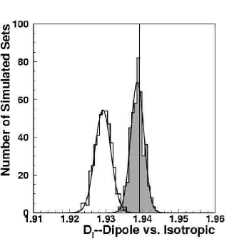
(b)

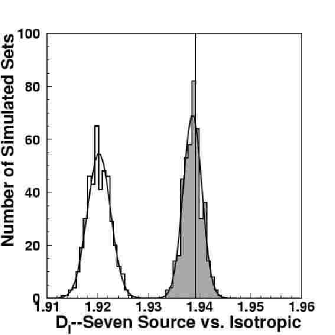
(c)

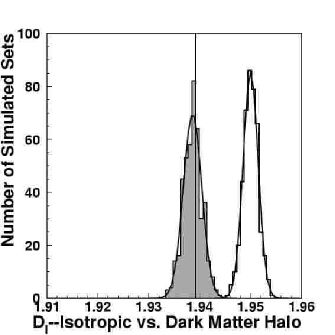
Figure 10: Comparison of distributions of $D_{\rm I}$ values for $\sim 500$ sets of 2000 events between the isotopic source model (shaded) and the other three source models — (a): Dipole enhancement model vs. Isotropic model $(\alpha=1.0)$; (b): Seven source model vs. Isotropic model $(F_{s}=0.28)$; (c): Isotropic model vs. Dark matter halo source model $(r_{s}=10~{}{\rm kpc})$. The vertical line corresponds to the value of $D_{\rm I}$ for the “real” 2000 event sample. In all cases the distributions of $D_{\rm I}$ values fit well to a Gaussian curve.

6 Application to Anisotropy Analysis

We now need to develop a scheme by which we can apply fractal dimensionality analysis to a real data set. In the case of a real data set, we will be dealing with only one value of $D_{\rm I}$. By itself $D_{\rm I}$ is insufficient to characterize the data set; $D_{\rm I}$ fluctuates a great deal due to variation in $N_{\rm Shower}$. However, a comparison between the value of $D_{\rm I}$ for a real event sample and a distribution of $D_{\rm I}$ values (with the same $N_{\rm Shower}$ and $N_{\rm Dist}$ values as the real data) for a series of simulated data sets of a given source model does provide a viable measurement of anisotropy.

We can demonstrate this by considering a single simulated event sample generated with an isotropic source model. We will suppose this sample to be our “real” data. We consider the isotropic simulated event samples shown in figures 7a and 8a. We will once again stipulate that $<\!\!n_{i}\!\!>=500$ which means that in the case of $N_{Shower}=500$, we have: $N_{\rm Dist}\simeq 1.6\times 10^{5}$ which leads to $D_{\rm I}=1.89715$ and in the case of $N_{Shower}=2000$, we have: $N_{\rm Dist}\simeq 4\times 10^{4}$ which leads to $D_{\rm I}=1.93920$.

In figures 9 and 10, we demonstrated that for a fixed scaling parameter the distribution of $D_{\rm I}$ values for a large number of simulated sets fits well to a Gaussian curve. By establishing the relationship between the distribution of $D_{\rm I}$ values and the scaling parameter in each model, we can establish a 90% confidence interval on the scaling parameter for that model.

6.1 Dipole Enhancement Source Model

In the case of the dipole enhancement source model in equation 17, the scaling parameter is $\alpha$. By varying $\alpha$ between $-1$ and $1$, we develop a curve which will show the relationship between $D_{\rm I}$ and $\alpha$. By considering the actual value of $D_{\rm I}$ for the “real” data set, we then establish a nominal value for $\alpha$ and a 90% confidence interval. The results for both $N_{Shower}=500$ and $N_{Shower}=2000$ are shown in figure 11. In the case of our simulated isotropic set with $N_{Shower}=500$, $\alpha=0.02\pm 0.21$ with a 90% confidence interval of $[-0.29,0.36]$. In the case of our simulated isotropic set with $N_{Shower}=2000$, $\alpha=0.075\pm 0.085$ with a 90% confidence interval of $[-0.065,0.24]$. These results tell us that our “real” data can, at the $1\sigma$ level of up to 0.2. We notice that in figure 11, there are potentially two suitable intervals of $\alpha$ that possess similar values of $D_{\rm I}$. This emphasizes the necessity of making density plots to assure by visual inspection that the appropriate interval is chosen.

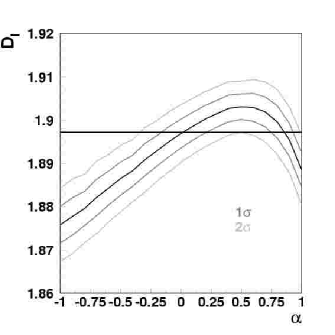
(a)	(b)
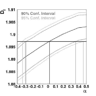
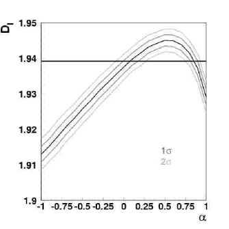
(c)	(d)

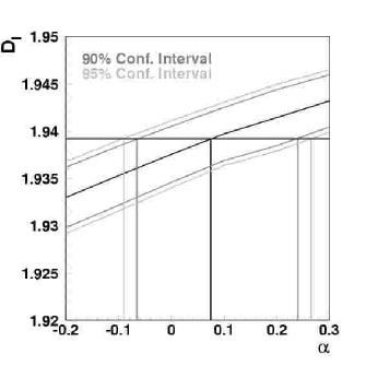
Figure 11: Study of the dependence of $D_{\rm I}$ upon $\alpha$ for a dipole enhancement source model—(a): $N_{Shower}=500$ $\alpha=.02\pm.21$; (b): $N_{Shower}=500$ (zoomed); 90% confidence interval: $[-0.29,0.36]$; (c): $N_{Shower}=2000$; $\alpha=.075\pm.085$; (d): $N_{Shower}=2000$ (zoomed); 90% confidence interval: $[-0.065,0.24]$. In each case, the solid solid horizontal line indicates the value of $D_{\rm I}$ for the simulated isotropic data set. The vertical lines in (b) and (d) indicate the projection of the nominal value and 90% and 95% confidence intervals of $\alpha$ on the $x$-axis.

6.2 Seven Source Model

In the case of the seven source model, the scaling parameter is $F_{s}$, the fraction of the total event sample that is produced by the discrete sources. By varying $F_{s}$ between $0$ and $0.40$, we develop a curve which shows the relationship between $D_{\rm I}$ and $F_{s}$. By considering the actual value of $D_{\rm I}$ for the “real” data set, we then establish a nominal value for $F_{s}$ and a 90% confidence upper limit for $F_{s}$. The results for both $N_{Shower}=500$ and $N_{Shower}=2000$ are shown in figure 12. In the case of our simulated isotropic set with $N_{Shower}=500$, we have a 90% confidence upper limit of $F_{s}=0.16$. In the case of our simulated isotropic set with $N_{Shower}=2000$, we have a 90% confidence upper limit of $F_{s}=0.04$. This tells us that our “real” data can have, at most, 16% (for 500 events) or 4% (for 2000 events) of these events coming from the seven sources.

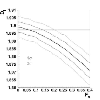
(a)	(b)
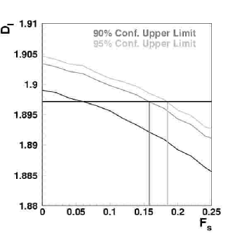
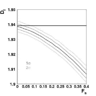
(c)	(d)

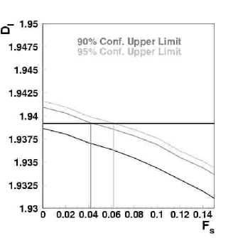
Figure 12: Study of the dependence of $D_{\rm I}$ upon $F_{s}$ for the seven source model—(a): $N_{Shower}=500$; (b): $N_{Shower}=500$ (zoomed); 90% confidence upper limit=0.16; (c): $N_{Shower}=2000$; (d): $N_{Shower}=2000$ (zoomed); 90% confidence upper limite=0.04;. In each case, the solid solid horizontal line indicates the value of $D_{\rm I}$ for the simulated isotropic data set. The vertical lines in (b) and (d) indicate the projection of 90% and 95% confidence upper limits of $r_{\rm s}$ on the $x$-axis.

6.3 Dark Matter Halo Source Model

In the case of the dark matter halo source model in equation 19, the variable parameter is $r_{\rm s}$, the critical radius in the NFW profile [19]. By varying $r_{\rm s}$ between $5.0$ kpc and $15.0$ kpc we develop the curve which will demonstrate the dependence of $D_{\rm I}$ upon $r_{\rm s}$. We can then show that the dark matter halo source model can be rejected with at level $\geq 3.6\sigma$ for $N_{Shower}=500$ and at a level of $\geq 7.0\sigma$ for $N_{Shower}=2000$ for the full range of hypothesized values for $r_{\rm s}$. The results are shown in figure 13.

(a)

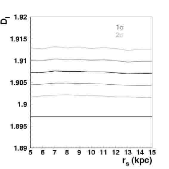
(b)

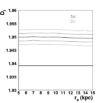
Figure 13: Comparison of the distribution of $D_{\rm I}$ values for a dark matter halo source model with a full range of hypothesized values for $r_{\rm s}$—(a): $N_{Shower}=500$, the dark matter halo model can be rejected at a level $\geq 3.6\sigma$; (b): $N_{Shower}=2000$, the dark matter halo model can be rejected at a level $\geq 7.0\sigma$. In each case, the solid horizontal line indicates the value of $D_{\rm I}$ for the simulated isotropic data set.

7 Discussion

Fractal dimensionality has several advantages over conventional anisotropy techniques. First of all, it naturally accommodates angular resolution. This is extremely important when considering event sets with asymmetric errors, when analysing event sets with variable values for the angular resolution (e.g. dependent on energy or geometry), or when combining multiple data sets from different detectors for a single analysis.

Another advantage that fractal dimensionality possesses is the ability to accommodate any aperture. Because this method makes a relative comparison between a sample and simulations using the same aperture, the physical aperture is simply folded into the analysis. This once again allows the combination of data from multiple detectors with very different apertures. It also allows the analysis of extremely complicated apertures without the need to include normalizing factors that needlessly complicate the predictability of the Poisson fluctuations in the data sample.

Perhaps the most striking feature of the fractal dimensionality method is that it only requires a single measurement of one’s data. While fractal dimensionality will not always provide better statistical significance than a direct measurement for a specific anisotropy, the fact that one considers only a single measurement of the data, for any number of potential anisotropic models, provides one the means to simultaneously reject or accept all of those models without the ensuing statistical penalty.

A possible way of increasing the sensitivity of the fractal dimensionality method is by considering the general case of case of $D_{q}$. By varying the value of $q$ to something other than $1$, it might be possible to increase the sensitivity of this method to various anisotropies.

The fractal dimensionality method does have some weaknesses. First and foremost is the potential for multiple solutions as was demonstrated in the dipole source model above. The method cannot be applied blindly. It requires a careful inspection of both the data sample and the simulated samples in order to resolve possible ambiguities. Another drawback is the amount of computation required to calculate $D_{\rm I}$ for a large number of simulated data sets. Producing just the plots in figure 11c consumed the equivalent of $\sim 1000$ CPU hours on 1GHz Athlon machine. Another limitation is the potential for different source models to effectively cancel each other out and yield a potentially deceiving value of $D_{\rm I}$ that resembles that of an isotropic source. One solution for this is to separately consider the value of $D_{\rm I}$ for different celestial regions in the data. Of course, this will incur a statistical penalty.

Two particularly useful roles for fractal dimensionality analysis are (a): as a first test to ascertain if a sample possesses the same heterogeneity as the expected isotropic background and (b): as a wholly independent observable that can be used to confirm the results of a direct measurement.

Today the HiRes detector continues to accumulate data. Soon the Auger detector will be acquiring data at seven times the rate of HiRes. As the number of observed UHECRs continues to rise, fractal dimensionality will grow ever more effective in its ability to discern the between potential source models in the continuing effort to solve the mystery of UHECRs.

8 Acknowledgments

This work is supported by US NSF grants PHY-9321949 PHY-9974537, and PHY-0140688. We would like to thank Professors Glennys Farrar and Benjamin Bromley for invaluable insights that went into the analysis used to produce this paper. We gratefully acknowledge the contributions from the University of Utah Utah Center for High Performance Computing.

References

- [1] M. Takeda et al., Astrophys. J. 522, 225 (1999) [arXiv:astro-ph/9902239].
- [2] J. Bellido et al., Proc. of 27th ICRC (Hamburg), 1, 364 (2001).
- [3] C. C. H. Jui et al., Proc. of 27th ICRC (Hamburg), 1, 354 (2001).
- [4] N. Hayashida et al., Proc. of 26th ICRC (Salt Lake City), 3, 256 (1999) [arXiv:astro-ph/9906056].
- [5] D. J. Bird et al., Proc. of 23rd ICRC (Calgary), 2, 51 (1993).
- [6] D. J. Bird et al., Proc. of 23rd ICRC (Calgary), 2, 30 (1993).
- [7] D. J. Bird et al., Ap. J. 511, 738 (1999) [arXiv:astro-ph/9806096].
- [8] T. Stanev et al., Phys. Rev. Lett. 75, 3056-3059 (1995) [arXiv:astro-ph/9505093].
- [9] A. N. Kolmogorov, Dokl. Akad. Nauk. SSSR 124, 754 (1959), Math. Rev. 21, 2035 (1959).
- [10] J. Balatoni and A. Reyni, Publ. Math. Inst. Hung. Acad. Sci. 1, 9 (1959).
- [11] A. H. Nayfeh and B. Balachandran, Applied Nonlinear Dynamics: Analytical, Computational, and Experimental Methods (Wiley, New York, 1995) pp. 545-547.
- [12] P. Grassberger, Phys. Lett. A 97, 227 (1983).
- [13] H. G. E. Hentschel and I. Procaccia, Physica D 8, 435, (1983).
- [14] T. Abu-Zayyad et al. [High Resolution Fly’s Eye Collaboration], arXiv:astro-ph/0208243.
- [15] T. Abu-Zayyad et al. [High Resolution Fly’s Eye Collaboration], arXiv:astro-ph/0208301.
- [16] D. J. Bird et al. [HIRES Collaboration], Astrophys. J. 424, 491 (1994).
- [17] M. Takeda et al., Phys. Rev. Lett. 81, 1163 (1998) [arXiv:astro-ph/9807193].
- [18] G. R. Farrar and T. Piran, arXiv:astro-ph/0010370.
- [19] J. F. Navarro, C. S. Frenk and S. D. M. White, Astrophys. J. 462, 563 (1996) [arXiv:astro-ph/9508025].