Detectability of Long GRB Afterglows from Very High Redshifts

Abstract

Gamma-ray bursts are promising tools for tracing the formation of high redshift stars, including the first generation. At very high redshifts the reverse shock emission lasts longer in the observer frame, and its importance for detection and analysis purposes relative to the forward shock increases. We consider two different models for the GRB environment, based on current ideas about the redshift dependence of gas properties in galaxies and primordial star formation. We calculate the observed flux as a function of the redshift and observer time for typical GRB afterglows, taking into account intergalactic photoionization and Lyman-$\alpha$ absorption opacity as well as extinction by the Milky Way Galaxy. The fluxes in the X-ray and near IR bands are compared with the sensitivity of different detectors such as Chandra, XMM, Swift XRT and JWST. Using standard assumptions, we find that Chandra, XMM and Swift XRT can potentially detect GRBs in the X-ray band out to very high redshifts $z\gtrsim$ 30. In the K and M bands, the JWST and ground-based telescopes are potentially able to detect GRBs even one day after the trigger out to $z\sim$ 16 and 33, if present. While the X-ray band is insensitive to the external density and to reverse shocks, the near IR bands provide a sensitive tool for diagnosing both the environment and the reverse shock component.

1 Introduction

Gamma-ray bursts are thought to be associated with the formation of massive stars (van Paradijs, Kouveliotou, & Wijers 2000). The evidence for this has been mainly in the class of long bursts, of $\gamma$-ray durations in excess of 2 seconds, making up two-thirds of the GRB population, which are the only ones so far for which X-ray, optical, IR and radio afterglows, as well as redshifts, have been measured. The strongest evidence yet comes from the recently confirmed association of long GRBs with core-collapse supernovae (Stanek et al. 2003; Hjorth et al. 2003; Uemura et al. 2003; Price et al. 2003). Short bursts, of durations less than 2 seconds, even if produced e.g. by neutron star mergers, would similarly be associated with massive star formation, and one expects the rate of occurrence of GRBs with redshift to follow closely the massive star formation rate. In currently favored $\Lambda$CDM cosmologies, star formation should start at redshifts higher than those where proto-galaxies and massive black holes at their centers develop (Miralda-Escudé 2003). Thus, GRBs could trace the pre-galactic star formation era preceding quasars.

Recent cosmic microwave background anisotropy data collected by WMAP reveal that the first objects in the Universe should be formed around $z\approx 18$ (Bennett et al. 2003). This is consistent with the theoretical modeling of the first star formation (Abel et al. 1998, 2000, 2002; Bromm et al. 1999). There is also indirect observational evidence for high-z GRBs. E.g., empirical relations have been found between the GRB luminosities and other measured quantities, such as the variability of the gamma-ray light curves (Fenimore & Ramirez-Ruiz 2000) and spectral lags (Norris et al. 2000). By extrapolating these empirical laws to a larger burst sample (e.g. the BATSE data), it is found that many BATSE bursts would be expected to have $z>6$ (Fenimore & Ramirez-Ruiz 2000).

The discovery of the highest redshift quasars, such as the current record holder at $z=6.43$ (Fan et al. 2003), grows increasingly difficult because the quasar formation rate drops rapidly at higher redshifts, peaking between redshift 2 and 3. Very few galaxies can be seen above $z>6$, which is also consistent with the upper limit for the redshift of galaxy formation $z_{gal}\leq 9$ based on theoretical analysis (e.g. Padmanadhan 2001). Although young galaxies may exist at very high redshifts, they are likely to be too faint to obtain good spectra (Haiman & Loeb 1997). On the other hand, the extreme brightness of GRBs during their first day or so make them the most luminous astrophysical objects in the Universe. Thus, GRBs appear to be promising tools to explore the very high redshift Universe (Miralda-Escudé, 1998).

The natural question which needs to be quantified is the degree of detectability of GRBs with current or future detectors, if they occur at much higher redshifts than those currently sampled. Lamb & Reichart (2000) used specific templates such as GRB 970228 observed at one day to estimate the highest redshifts at which such bursts could be observed using Swift. Ciardi & Loeb (2000) calculated the flux evolution with redshift of common GRBs and discussed the flux change with redshift at several epochs in the infrared bands. These papers considered only forward shock radiation as known before 2000 and some effects of the galactic mean density evolution but did not consider the primeval star-formation environment.

In this paper we have calculated the flux evolution of typical GRBs based on current knowledge about GRB physics in a more realistic way. Among the refinements introduced are: (1) The contribution from reverse shocks is considered as a crucial element. This should be very important for the early afterglow in the rest-frame (which at high redshifts gets dilated to longer observed times). Therefore, we expect that at higher redshifts the possibility of observing the reverse shock is much increased. (2) We have taken up to date GRB parameters, e.g. incorporating new estimates of the typical magnetic equipartition parameter $\epsilon_{B}$ about one order or more magnitude smaller than the electron parameter $\epsilon_{e}$ in the forward shock, and a possibly higher $\epsilon_{B}$ in the reverse shock. This has a significant effect on the GRB evolution. (3) We consider GRB external densities motivated both by views on the typical protogalaxy density evolution with redshift, and by views on the conditions around the first stars to form in the universe in the pre-galactic era. (4) We consider both the Lyman-$\alpha$ and photoionization absorption as well as our own galactic extinction. (5) We compare the expected fluxes in the X-ray and near IR bands to the sensitivity of various detectors such as Chandra, XMM, Swift XRT and JWST.

In §§2.1 and 2.2 we outline the basic forward and reverse shock flux calculations, the details of which are given in an appendix. We discuss the GRB density environment in §2.3, and the intergalactic and galactic absorption effects are estimated in §2.4. In §§3.1 and 3.2 we discuss the optical/IR and X-ray flux dependence on redshift, respectively, at various observer times, including the dependence on external density. We compare these to the Swift XRT, Chandra, XMM and JWST sensitivities for the detection of GRBs at different redshifts. We summarize the numerical results and discuss the implications in §4.

2 Afterglow characteristics

2.1 Forward Shock

We assume that the shock-accelerated electrons have a power-law distribution of Lorentz factors $\gamma_{e}$ with a minimum Lorentz factor $\gamma_{m}$: $N(\gamma_{e})d\gamma_{e}\propto\gamma_{e}^{-p}d\gamma_{e},\gamma_{e}\geq\gamma_{m}$. We also define a critical Lorentz factor $\gamma_{c}$ above which the electrons cool radiatively on a time shorter than the expansion time scale (Mészáros, Rees, & Wijers 1998). This leads to the standard (forward shock) broken power law spectrum of GRBs (Sari, Piran, & Narayan 1998). In the fast-cooling regime, when $\gamma_{m}>\gamma_{c}$, all the electrons cool rapidly down to a Lorentz factor $\approx\gamma_{c}$ and the observed flux at frequency $\nu$ is

$$F_{\nu}=F_{\nu,m,f}\left\{\begin{array}[]{l@{\quad\quad}l}(\nu/\nu_{c,f})^{1/3}&\nu<\nu_{c,f}\cr(\nu/\nu_{c,f})^{-1/2}&\nu_{c,f}\leq\nu<\nu_{m,f}\cr(\nu_{m,f}/\nu_{c,f})^{-1/2}(\nu/\nu_{m,f})^{-p/2}&\nu_{m,f}\leq\nu\end{array}\right.$$ (1)

Hereafter the subscripts ‘f’ and ‘r’ indicate forward and reverse shock, respectively.

In the slow-cooling regime, when $\gamma_{c}>\gamma_{m}$, only electrons with $\gamma_{e}>\gamma_{c}$ cool efficiently, and the observed flux is

$$F_{\nu}=F_{\nu,m,f}\left\{\begin{array}[]{l@{\quad\quad}l}(\nu/\nu_{m,f})^{1/3}&\nu<\nu_{m,f}\cr(\nu/\nu_{m,f})^{-(p-1)/2}&\nu_{m,f}\leq\nu<\nu_{c,f}\cr(\nu_{c,f}/\nu_{m,f})^{-(p-1)/2}(\nu/\nu_{c,f})^{-p/2}&\nu_{c,f}\leq\nu\end{array}\right.$$ (2)

where $F_{\nu,m,f}$ is the observed peak flux at the observed frequency $\nu=\min(\nu_{c,f},\nu_{m,f})$, while $\nu_{m,f}$ and $\nu_{c,f}$ are the observed frequencies corresponding to $\gamma_{m}$ and $\gamma_{c}$, respectively. Synchrotron self-absorption can also cause an additional break at very low frequencies, typically about $\leq 5\ {\rm GHz}$, in the radio range. Since here we focus on the IR and X-ray ranges, we will not consider this low-frequency regime in our calculations. For a fully adiabatic shock, the evolution of the typical frequency and peak flux are given by Sari et al. (1998):

$$\nu_{c,f} = 2.5\times 10^{12}\epsilon_{B,f}^{-3/2}E_{52}^{-1/2}n^{-1}t_{5}^{-1/2}\times(1+z)^{-1/2}\ {\rm Hz},$$ (3)

$$\nu_{m,f} = 4.6\times 10^{14}\epsilon_{B,f}^{1/2}\epsilon_{e}^{2}E_{52}^{1/2}t_{5}^{-3/2}\times(1+z)^{1/2}\ {\rm Hz},$$ (4)

$$F_{\nu,m,f} = 1.1\times 10^{5}\epsilon_{B,f}^{1/2}E_{52}n^{1/2}D_{28}(z)^{-2}\times(1+z)\ {\rm\mu Jy~{}}.$$ (5)

Hereafter the quantities without the subscript ‘s’ are in the observer frame, and the quantities with the subscript ‘s’ are for the observer in the local frame of the source, which is connected with the observer frame quantities with a certain power of $(1+z)$. The source is assumed at a luminosity distance $D_{L}(z)=10^{28}D_{28}(z)$ cm, and $\epsilon_{B}$ and $\epsilon_{e}$ are the fraction of the shock energy converted into energy of magnetic fields and accelerated electrons, respectively. The time is taken in units of $t=10^{5}t_{5}$ s ($\simeq$ 1 day), $E_{52}=E/10^{52}\ {\rm ergs}$ is the isotropic equivalent energy of the GRBs, and $n$ is the particle density in units of ${\rm cm^{-3}}$ in the ambient medium around the GRB.

2.2 Reverse Shock

As GRBs are measured at increasingly larger redshifts, a given constant observer time corresponds to increasingly shorter source frame times. This is favorable for observing at very high redshifts the evolution of phenomena which happen only in the earliest stages of the GRB, such as the reverse shock emission. So far, the reverse shock emission has been observed in only three GRBs in the optical band: GRB 990123 (Akerlof et al. 1999), GRB 021004 (Fox et al. 2003a) and GRB 021211 (Fox et al. 2003b; Li et al. 2003). At these early epochs, the reverse shock emission makes a significant contribution to the overall flux of the GRB afterglow. A description of the reverse shock spectrum is however more complicated than that of the forward shock. It depends on two factors: (1) whether one is in the thick shell or thin shell case, and (2) the ratio of the crossing time of the reverse shock across the shell to the observing time. We consider a relativistic shell with an isotropic equivalent energy $E$ and initial Lorenz factor $\eta\equiv L_{\gamma}/{\dot{M}}c^{2}$ expanding into a homogeneous interstellar medium of particle number density $n$. In the local frame, we can define a deceleration timescale when the accumulated ISM mass is $1/\eta$ of the ejecta mass, $t_{dec,s}=[(3E/4\pi\eta^{2}nm_{p}c^{2})^{1/3}/2\eta^{2}c]$, which is the conventional deceleration timescale. A critical initial Lorenz factor $\eta_{c}$ can be defined by the condition that the deceleration time $t_{dec,s}$ equals the intrinsic (i.e. central engine dominated) duration $T_{s}$ of the gamma-ray burst, which is $\eta_{c}\simeq 228.6E_{52}^{1/8}n^{-1/8}T_{s,1}^{-3/8}$. The thick shell case occurs when the duration $T_{s}>t_{dec,s}$, and the thin shell case occurs when $T_{s}<t_{dec,s}$. The time taken by the reverse shock to cross the shell is defined as $t_{\times,s}=\max(t_{dec,s},T_{s})$. In the observer frame, $t_{\times}=t_{\times,s}(1+z)$. For observation times $t<t_{\times}$, the reverse shock emission spectrum qualitatively resembles the forward shock spectrum. However, for $t>t_{\times}$, we take the approximation that there is no reverse shock emission above $\nu_{c,r}$, since all electrons have cooled below that energy. Thus the reverse shock spectrum at $t>t_{\times}$ is, in the fast cooling case

$$F_{\nu}=F_{\nu,m,r}\left\{\begin{array}[]{l@{\quad\quad}l}(\nu/\nu_{c,r})^{1/3}&\nu<\nu_{c,r}\cr 0&\nu_{c,r}\leq\nu<\nu_{m,r}\cr 0&\nu_{m,r}\leq\nu\end{array}\right.$$ (6)

In the slow cooling case the reverse shock spectrum is

$$F_{\nu}=F_{\nu,m,r}\left\{\begin{array}[]{l@{\quad\quad}l}(\nu/\nu_{m,r})^{1/3}&\nu<\nu_{m,r}\cr(\nu/\nu_{m,r})^{-(p-1)/2}&\nu_{m,r}\leq\nu<\nu_{c,r}\cr 0&\nu_{c,r}\leq\nu\end{array}\right.$$ (7)

where $\nu_{c,r},\nu_{m,r}$ and $F_{\nu,m,r}$ refer here to the reverse shock cooling frequency, typical frequency and peak flux, respectively. Since these quantities are usually different in the reverse and in the forward shocks, and have different functional forms and time evolution dependences in the thick and thin shell cases, the specific shock and shell cases will be differentiated in the treatment below.

Kobayashi (2000) has given expressions of cooling frequency, typical frequency of electrons and peak flux in the reverse shock. Motivated by recent observations of prompt flashes, a set of relations linking the cooling frequency, typical frequency and peak flux in the reverse and forward shocks at the crossing time was proposed by Kobayashi & Zhang (2003) and Zhang, Kobayashi, & Mészáros (2003). The flux calculated with these two different sets of formulae are consistent within a 10% error range. Here we use the relationships as discussed in the last two quoted references,

$$\frac{\nu_{m,r}(t_{\times})}{\nu_{m,f}(t_{\times})}=(\gamma_{\times}^{2}/\eta)^{-2}{\cal R_{B}}\;\;,\;\;\frac{\nu_{c,r}(t_{\times})}{\nu_{c,f}(t_{\times})}={\cal R_{B}}^{-3}\;\;,\;\;\frac{F_{\nu,m,r}(t_{\times})}{F_{\nu,m,f}(t_{\times})}=(\gamma_{\times}^{2}/\eta){\cal R_{B}}$$ (8)

where

$$\gamma_{\times}=\min(\eta,\eta_{c})~{}~{}~{},{\rm and}~{}~{}~{}{\cal R_{B}}\equiv B_{r}/B_{f}=\left(\epsilon_{B,r}/\epsilon_{B,f}\right)^{1/2}.$$ (9)

Here $\cal R_{B}$ reflects a possible stronger B field in reverse shock, as inferred from the analyses of the GRB 990123 and GRB 021200 data (Zhang et al. 2003). In our calculations we set ${\cal R_{B}}=1$ as the standard case, and take ${\cal R_{B}}=5$ as an alternative option. As an example, when the observer time is larger than the crossing time, $t\geq t_{\times}$=max($T,t_{dec}$), i.e. the fast cooling case, the observed cooling frequency, typical frequency and peak flux of the reverse shock are

$$\nu_{c,r} = (t_{\times}/t)^{3/2}{\cal R_{B}}^{-3}\nu_{c,f}(t_{\times})=2.5\times 10^{12}\epsilon_{B,r}^{-3/2}E_{52}^{-1/2}n^{-1}t_{5}^{-3/2}t_{\times,5}\times(1+z)^{-1/2}{\cal R_{B}}^{-3}\ Hz,$$

$$\nu_{m,r} = \gamma_{\times}^{-4}\eta^{2}(t_{\times}/t)^{3/2}{\cal R_{B}}\nu_{m,f}(t_{\times})=4.6\times 10^{14}\gamma_{\times}^{-4}\eta^{2}\epsilon_{B,r}^{1/2}\epsilon_{e}^{2}E_{52}^{1/2}t_{5}^{-3/2}\times(1+z)^{1/2}{\cal R_{B}}\ Hz,$$ (10)

$$F_{\nu,m,r} = \gamma_{\times}^{2}\eta^{-1}(t_{\times}/t){\cal R_{B}}F_{\nu,m,f}(t_{\times})=1.1\times 10^{5}\epsilon_{B,r}^{1/2}E_{52}n^{1/2}D_{28}(z)^{-2}\times(1+z)\gamma_{\times}^{2}\eta^{-1}t_{\times,5}t_{5}^{-1}{\cal R_{B}}\ \mu Jy.$$

In the appendix we give further details of the expressions for the flux evolution of the forward and reverse shocks in the thin and thick shell as well as in the fast or slow cooling cases.

2.3 GRB density environment

The typical environments considered for GRBs are either the (approximately) constant number density case $n_{0}\sim$ constant (i.e. independent of the distance $r$ from the center for the burst), or a power law dependence as might be expected in the stellar wind from the progenitor, e.g. $n\propto r^{-2}$ (Mészáros et al. 1998; Dai & Lu 1998; Chevalier & Li 1999; Whalen, Abel, & Norman, 2003). In our calculation, for simplicity we consider only the first case of $n\sim$ constant, which appears to satisfy most of the observed cases that have been analyzed (Panaitescu & Kumar 2001,2002; Frail et al. 2001). While this density is different for different bursts, we can assume a typical average value $n_{0}$ for $n$ at redshift $z=1$. One has to consider then how this typical density might evolve with redshift. We concentrate on two very different types of dependencies, motivated by different physics. (1) Based on hierarchical models of galaxy formation (Kauffmann, White, & Guiderdoni 1993; Mo, Mao, & White 1998), the mass and size of galactic disks is expected to evolve with redshift (Barkana & Loeb 2000). For a fixed host galaxy mass, this yields $n(z)=n_{0}(1+z)^{4}$ (Ciardi & Loeb 2000). (2) Recent numerical simulations of primordial star formation indicate that the particle number density around the first stars at very high redshift could be in the range $1\lesssim n_{0}\lesssim 10^{-2}$ cm^-3 (Whalen et al. 2003), approximately independent of redshift because of strong radiation pressure from the central massive star, which dominates and smooths any variations in the original galactic number density around the stars. The size scale of this region of dominance is about several parsecs, which is $\gtrsim$ the length scale of typical afterglows. Here we assume that, for this case (2), this stellar dominance applies to all GRBs originating from massive stars, so the number density in the relevant region around the GRB is the same constant at all redshifts, i.e. $n(z)=n$. Thus, the two density cases considered are

$$n(z)=n_{0}\times\left\{\begin{array}[]{l@{\quad\quad}l}(1+z)^{0}&\hbox{constant density model}\\ (1+z)^{4}&\hbox{density evolution model}\end{array}\right.$$ (11)

Here $n_{0}$ is normalized by $n_{0}=1$ cm^-3 at $z=1$, noting that uncertainties in the primordial star calculations could make this as low as $10^{-2}$ cm^-3. This number density $n$ refers to the local ISM density in the immediate neighborhood of the burst.

2.4 Intergalactic and galactic absorption

As it propagates through the intergalactic medium (IGM), the afterglow radiation from a burst occurring at some redshift $z$ is subject to several absorption processes. The most important are Lyman-$\alpha$ absorption, photoionization of neutral hydrogen, and photoionization of He II. At very high redshifts, before the intergalactic medium becomes re-ionized, which may be taken to occur between the limits $z_{i}\gtrsim 6.3$ (Fan et al. 2001; Miralda-Escudé 2003; Onken & Miralda-Escudé 2003) and $z_{i}\sim 17\pm 5$ (Spergel et al. 2003), most of the mass as well as most of the volume of the IGM is in the form of neutral gas. At redshifts below this, after re-ionization by the first stars or galaxies, an increasing fraction of the IGM volume becomes ionized, interspersed with clouds of neutral gas associated with the halos of protogalaxies, which continue to absorb radiation. The exact distribution of clouds as a function of redshift is not well known, but estimates of the effective number are obtained by counting the numbers of absorption line systems in quasar spectra. These are used for calculating the effective absorption optical depth at redshifts below the reionization redshift. Below the reionization redshift, the photoionization opacity by HI is given by Madau, Haardt, & Rees (1999), based on the observed absorber distribution in the spectra of high-redshift quasars. The Lyman-$\alpha$ absorption optical depth can be obtained in a similar way. Above the reionization redshift, both the photoionization and Lyman-$\alpha$ opacities are obtained by means of an integration through the neutral gas between the reionization redshift and the redshift at which the GRB is located (Barkana & Loeb 2001).

At high redshifts, intergalactic He II becomes important at rest-frame energies $\gtrsim 54.4$ eV, where the effects of hydrogen photoionization are still important (Perna & Loeb 1998). However, the combined effect of the cross sections and the abundances, as well as the hardness of the ionizing spectra combine together to make He II the dominant opacity at observed photon energies $h\nu\gtrsim 54.4\hbox{eV}/(1+z)$ for sources located at $z\gtrsim 3$ (Miralda-Escudé 2001). Bluewards of this energy, as the cross section drops as $\nu^{-3}$, He II photoionization is the last process to become optically thin, and is therefore the dominant IGM constituent which determines the re-emergence of the source spectrum at frequencies above the blue end of the Gunn-Peterson trough. Adopting current values of the cosmological parameters, this occurs (Mészáros & Rees 2003) at soft X-ray energies of $h\nu_{t}\sim 0.2$ keV or $\nu_{t}\sim 5\times 10^{16}$ Hz.

Absorption by our own galaxy also becomes important in the UV and soft X-ray band. The combined cross section including galactic metals $\sigma_{ph}$ is given by Morrison & McCammon (1983). The optical depth is given by $\tau=\sigma_{ph}N_{H,Galaxy}$, where $N_{H,Galaxy}$ is the equivalent column density along the line of sight, which varies depending on the galactic latitude. Here we set the column density to be $2\times 10^{20}$ cm^-2, typical of moderately high latitudes, which becomes optically thin at energies $\gtrsim 0.2$ keV, comparable to the effects discussed above for the intergalactic He II.

Thus, one expects that between the Lyman-$\alpha$ frequency corresponding to the source frame and approximately $5\times 10^{16}$ Hz (below which the galactic extinction for the above column density becomes large), the flux observed from a high redshift GRB will be totally suppressed. Outside this range, the observed flux is much less affected by the intergalactic and galactic absorption.

3 Initial Conditions and Numerical Results

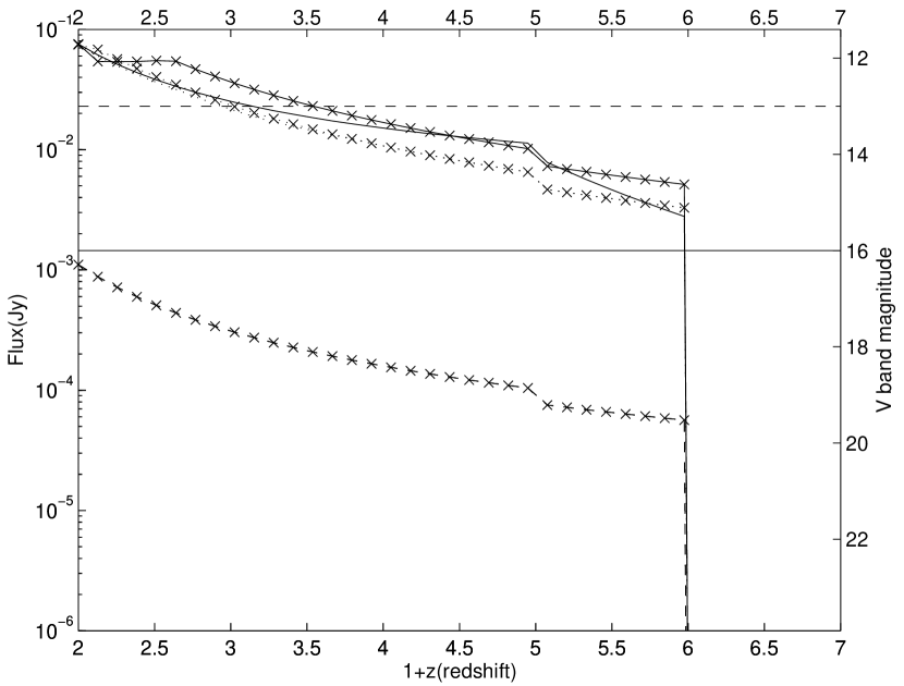
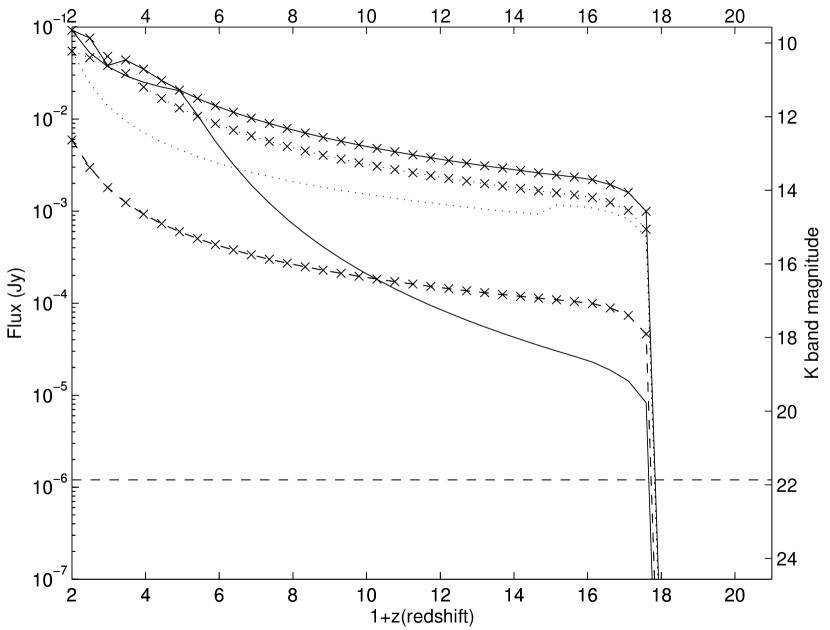
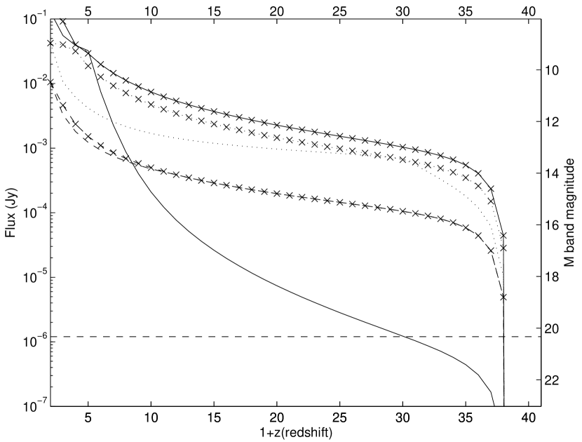
Figure 2: Combined forward and reverse shock observed flux as a function of redshift for $\epsilon_{B,f}=0.025$ and ${\cal R}_{B}=B_{r}/B_{f}=1$. Forward shock (symbols), reverse shock (without symbols). Solid, dashed and dotted lines indicate emission at different observer times t=10 mins, t=2 hour and t=1 day respectively. a): V-band ($\nu=5.45\times 10^{14}$ Hz); b): K-band ($\nu=1.36\times 10^{14}$ Hz); c): M-band ($\nu=6.3\times 10^{13}$ Hz). Straight lines: In V band sensitivities are for ROTSE at very early and late times; in K and M bands sensitivities for JWST K & M bands are estimated for a resolution R=1000, S/N=10 and integration time of 1 hour. Parameters: $n=1\ {\rm cm^{-3}},\epsilon_{e}=0.1,E_{52}=10,p=2.5,\eta=120.$

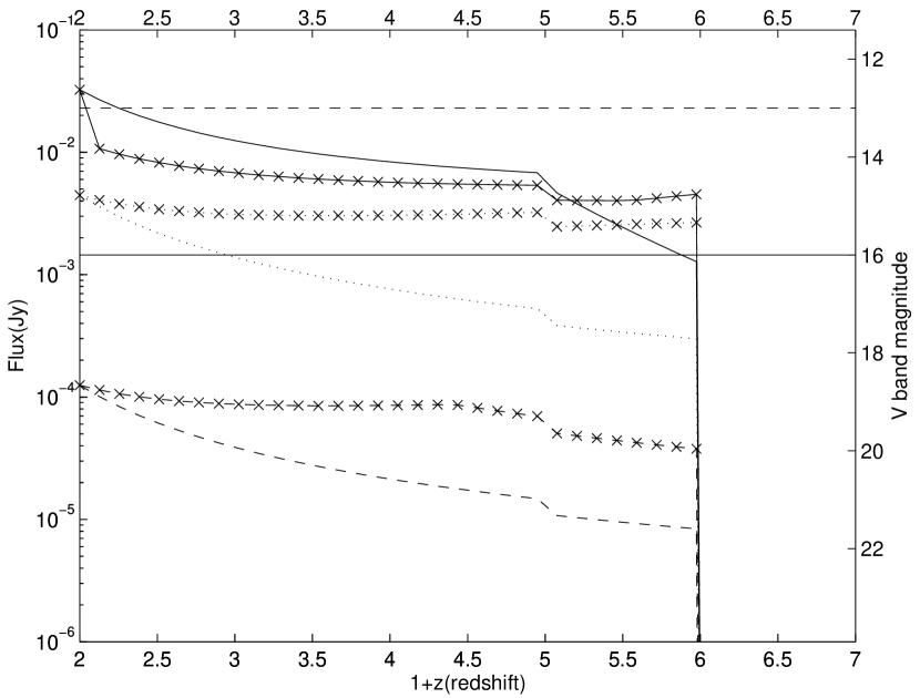
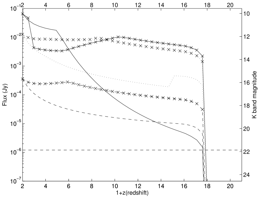
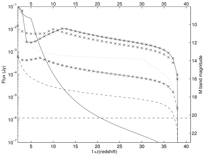
Figure 3: Combined forward and reverse shock observed flux as a function of redshift for the two density profiles $n=n_{0}=$ constant ( without symbols) and $n=n_{0}(1+z)^{4}$ (symbols) with $n_{0}=1$ cm^-3. solid, dashed and dotted lines indicate emission at different observer times t=10 mins, t=2 hour and t=1 day respectively. a): V-band ($\nu=5.45\times 10^{14}$ Hz); b): K-band ($\nu=1.36\times 10^{14}$ Hz); c): M-band ($\nu=6.3\times 10^{13}$ Hz). The limiting ROTSE and JWST sensitivities are the same as in Figure 2. Parameters: $\epsilon_{B,f}=0.001,{\cal R}_{B}=B_{r}/B_{f}=5,\epsilon_{e}=0.1,E_{52}=10,p=2.5,\eta=120.$

In our calculations, the nominal GRB parameter values adopted are an isotropic-equivalent energy $E_{52}=10$, shock parameters $\epsilon_{e}=0.1$, $\epsilon_{B,r}=0.025$, the ratio of magnetic field strength in reverse and forward shocks ${\cal R_{B}}=B_{r}/B_{f}=$ 1 or 5 ($\epsilon_{B,f}=0.025$ or $\epsilon_{B,f}=0.001$, respectively), and an initial Lorentz factor $\eta=120$. The GRB duration is assumed to be $T_{s}=10$ s in the source frame. The deceleration time $t_{dec,s}=[(3E/4\pi\eta^{2}nm_{p}c^{2})^{1/3}/2\eta^{2}c]$ in the source frame is determined mainly by GRB intrinsic parameters, except for the external ISM density $n$, which can depend on redshift in one of the scenarios considered. Substituting the parameters for $t_{dec,s}$, we have $t_{dec,s}=119.6n^{-1/3}\hbox{seconds}$. Therefore, for the $n$=const scenario, the reverse shock is exclusively in the thin shell case; for $n\propto(1+z)^{4}$ scenario the reverse shock will be in the thin shell case below some redshift, and above that redshift it will be in the thick shell case. We take a specific case where the reionization redshift of the Universe is at $z_{i}=15$, compatible with the WMAP value of Spergel et al (2003). As examples, we considered the burst properties at various observer’s times, e.g. 10 minutes, 2 hours and 1 day. The results are presented in Figs. 2 and 3, discussed below.

3.1 Light Curve

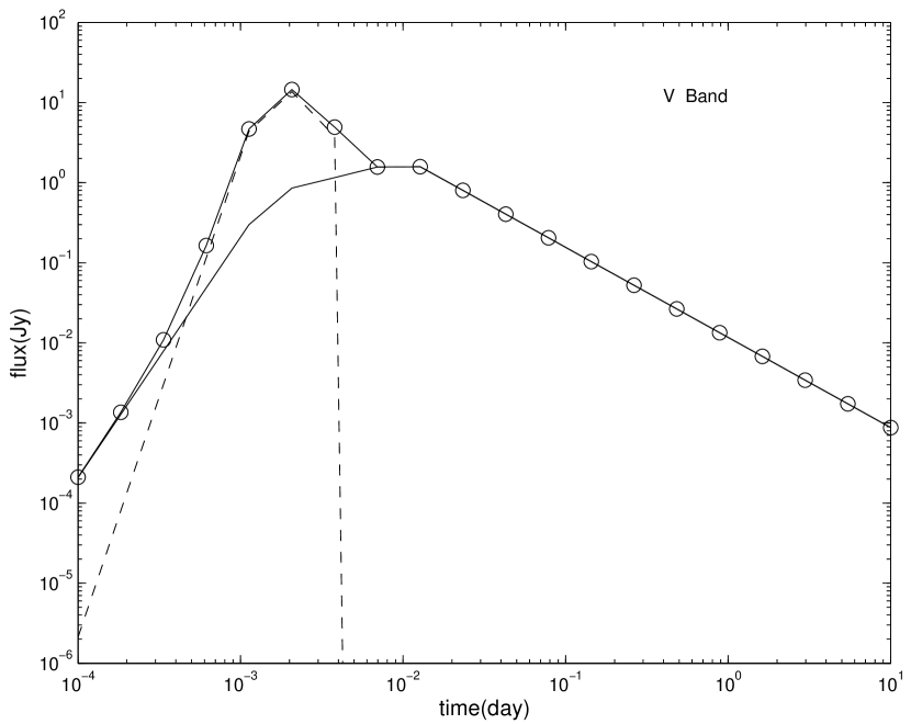
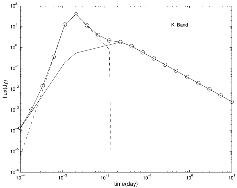
Figure 1: Typical light curves, for a redshift $z=1$. Reverse shock emission (dashed), forward shock emission (solid). total flux (symbols). Parameters:$\epsilon_{B,f}=0.001,{\cal R}_{B}=B_{r}/B_{f}=5,\epsilon_{e}=0.1,E_{52}=10,p=2.5,\eta=120,n_{0}=1\ {\rm cm^{-3}}$. a): V band ($\nu=5.45\times 10^{14}$ Hz); b): K band ($\nu=1.36\times 10^{14}$ Hz).

To show the distinct effects of the reverse and the forward shock on the flux behavior, we show the light curves for two different observational bands, V and K, here taken at a nominal redshift $z=1$. (Figure 1). As can be seen, the light curve evolution can be divided into 3 stages: (1) Forward shock dominant, before the reverse shock peaks. The timescale for this stage is relatively short. (2) Reverse shock dominant, after the reverse shock emission, which increases very quickly, exceeds the forward shock emission. The flux peaks when the reverse crosses the fireball shell. (3) Forward shock dominant. In this stage, after the reverse shock peak, the reverse shock emission decays very quickly and falls below the forward shock, so the forward shock is again dominant.

3.2 Infrared Flux Redshift Dependence

To test the self consistency of the code with the present optical observation like ROSTE, we plot the light curves in V band (Figures 2(a) and 3(a)). On these two figures the dashed an solid lines correspond to the sensitivities of ROTSE at very early and late times, respectively. The light curves show that we don’t expect to see many optical flashes, especially for high-$z$ GRBs. This is consistent with the present observations.

From the flux evolution equations (see appendix), it is seen that in the regime where the observing frequency is above the cooling frequency, $\nu>\nu_{c,f}$, the observed flux for the forward shock component is independent of the ISM number density (see (A4) & (A5)). We can define a critical redshift $z_{c}$, such that for $z>z_{c}$ the GRB afterglows for the forward shock component are in the density-independent regime (see eq.(3)).

$$(1+z_{c}) = 3.4\times 10^{2}(\epsilon_{B,f}/0.01)^{-3}E_{52}^{-1}n^{-2}t_{5}^{-1}(\lambda/2.2\mu\hbox{m})^{2}$$ (12)

$$= 1.1\times 10^{2}(\epsilon_{B,f}/0.01)^{-3}E_{52}^{-1}n^{-2}t_{5}^{-1}(1\hbox{eV}/h\nu)^{-2}$$

From the above equation (12), we see that the dependence of $z_{c}$ on $\epsilon_{B,f}$ is very sensitive, $\propto\epsilon_{B,f}^{-3}$. If we set $\epsilon_{B,f}=0.1$, we obtain the equations given by Ciardi & Loeb (2000). Taking $\epsilon_{B,f}$ smaller, the redshift $z_{c}$ can increase substantially. That is one of the main reasons why our curve of flux vs. redshift differs from that of Ciardi and Loeb (2000).

For the description of reverse shocks there are four relevant cases, depending on whether one is in the thin or thick shell limit, and on whether the times considered are before or after the shock crossing time. However, the cooling frequency evolution can be approximated by $\nu_{c,r}\propto t^{-3/2}$ for observer times $t>t_{\times}=\max(t_{dec},T)$. Also, if the observed frequency is larger than the cooling frequency $\nu\geq\nu_{c,r}$, the reverse shock emission disappears. Hence, we can define another critical redshift $z_{r}$ at which the reverse shock emission disappears,

$$(1+z_{r})=3.33\times 10^{-6}(\epsilon_{B,r}/0.01)^{-3}E_{52}^{-1}n^{-2}(t_{\times}/10\hbox{s})^{2}t_{5}^{-3}(\lambda/2.2\mu\hbox{m})^{2}{\cal R_{B}}^{-6}$$ (13)

which is a lower limit for $n\propto(1+z)^{4}$ and is an upper limit for $n=n_{0}=$constant, i.e. for $z\geq z_{r}$ when $n\propto(1+z)^{4}$ or for $z\leq z_{r}$ when $n$=const, there is no reverse shock emission (see below).

The two critical redshifts can be connected by the relations $\nu=\nu_{c,r}=(t_{\times}/t)^{3/2}{\cal R_{B}}^{-3}\nu_{c,f}(z_{r})$ and $\nu=\nu_{c,f}(z_{c})$. Cancelling out $\nu$ and substituting the expression for $\nu_{c,f}$, we obtain the relation

$$(1+z_{r})=(t_{\times}/t)^{3}{\cal R_{B}}^{-6}(1+z_{c}),$$ (14)

and we have the inequality

$$z_{r}<z_{c}$$ (15)

since ${\cal R_{B}}\geq 1$, and $t>t_{\times}$ by default, i.e. $z_{r}$ is defined for $t>t_{\times}$.

Using the parameters above and an observer frequency $\nu=1.36\times 10^{14}$ Hz ($6.3\times 10^{13}$ Hz) or $\lambda=2.2\ \mu$m ($4.8\ \mu$m), corresponding to the K-band (M-band) at observer times $t=10$ mins, 2 hour and 1 day, we have (${\cal R_{B}}=1$)

$$z_{r}=\cases{2.2,~{}0.1,~{}0~{}(3.0,~{}0.4,~{}0)&for $n\propto(1+z)^{4}$ ;\cr 0,~{}120.6,~{}\infty~{}(0,~{}24.5,~{}\infty)&for $n=1~{}\hbox{cm}^{3}$ .\cr}$$ (16)

From equation (2.2) we have, for the $n\propto(1+z)^{4}$ case,

$$\nu_{c,r,evolv}=2.5\times 10^{12}\epsilon_{B,r}^{-3/2}E_{52}^{-1/2}n_{z=0,evolv}^{-1}t_{5}^{-3/2}t_{dec,s,5}\times(1+z)^{-7/2}{\cal R_{B}}^{-3}\hbox{Hz}\propto(1+z)^{-29/6},$$ (17)

and for the $n=const$ case

$$\nu_{c,r,const}=2.5\times 10^{12}\epsilon_{B,r}^{-3/2}E_{52}^{-1/2}n_{z=0,const}^{-1}t_{5}^{-3/2}t_{dec,s,5}\times(1+z)^{1/2}{\cal R_{B}}^{-3}\hbox{Hz}\propto(1+z)^{1/2}.$$ (18)

From equations (13),(17),(18), we find some interesting differences between the two density profile cases. We discussed that for $\nu>\nu_{c,r}$ there is no emission from the reverse shock. However, the above behavior of $\nu_{c,r,evolv}\propto(1+z)^{-29/6}$ for $n\propto(1+z)^{4}$ and $\nu_{c,r,const}\propto(1+z)^{1/2}$ for the $n=n_{0}=$ constant case has some other consequences. For the same burst parameters, if there is no reverse shock emission at some observer time $t$ for $z=0$, in the $n\propto(1+z)^{4}$ case this implies that there will be no reverse shock emission at this same observer time at any redshift. For the $n=$ constant case, however, the chances are that the reverse shock emission will be observable above some redshift, because $\nu_{c,r,const}$ increases with redshift. This is caused by the effect of time dilation increasing as the redshift increases, which means that the same observer-frame time corresponds to earlier and earlier source-frame times. In the $n\propto(1+z)^{4}$ case, $\nu_{c,r,evolv}\propto(1+z)^{-29/6}$, and we can expect that $\nu_{c,r}$ will decay with $z$ quickly below $\nu$ even if $\nu_{c,r}$ is much larger than $\nu$ at low redshift. So, in this case, we can only observe the reverse shock emission at relatively low redshifts. On the other hand, in the $n=$ constant case we can observe the reverse shock emission at all redshifts if there is emission at low redshifts. We can see this from the fluxes in figure 2. If we substitute the values for the relevant parameters, we get $z\leq z_{r}=2.1$ and $z\leq z_{r}=0$ at $t=10$ mins and $t=1$ hour respectively for the $n\propto(1+z)^{4}$ case, whereas for the $n=const$ case, $z\geq z_{r}=0$ and $z\geq z_{r}=1975$ for those two corresponding times, and the emission from the reverse shock is observable in K band. This property provides one way of distinguishing these two different density profile regimes, based on the redshift distribution of the occurrence or absence of a reverse shock component.

From equations (14,15) we see that if $t>t_{\times}$ for the $n\propto(1+z)^{4}$ case, the reverse shock emission is absent already at redshifts lower than those beyond which the GRB emission would be in the density-independent regime. On the contrary, for the $n$=const case, reverse shock emission exists when the GRB emission is in the density-independent regime. Using this characteristic, we can again constrain the density profile around the GRBs.

Looking at Figure 2 which is the standard case of ${\cal R_{B}}=1$ in our calculation, several features can be noted: (1) At early times, e.g. $t=10\ {\rm mins}$ and $t=2$ hour, we can differentiate the constant density profile from the evolving density profile in both K and M bands. However, at late times it becomes difficult to do so in both bands, although the total flux in M band are somewhat different for both density profiles at relatively low redshifts. (2) For early observer times, e.g. $t=10\ {\rm mins}$, the amplitude of the total flux in the evolving density $n\propto(1+z)^{4}$ case at low redshifts shows some pronounced and complicated changes with redshift, as opposed to a more monotonous behavior in the constant density case. The changes in the former are caused by the transitions from one regime to another by the forward shock. Because in the evolving density example reverse shock emission disappearance above some very low redshift, over the redshift considered here forward shock emission component is dominant. On the other hand, in the constant density case, over the entire redshift range considered reverse shock emission is dominant. (3) The break in the light curve for the $n=$ constant case at $t=10$ minutes is caused by the transition from $t>t_{\rm dec,s}$ to $t<t_{\rm dec,s}$. (4) There is a sharp decline in the emitted flux in light curves at redshift $z\sim~{}17$ for K band and at $z\sim 36$, which are caused by the lyman-$\alpha$ and photoionization absorption of neutral hydrogen in IGM.

We also considered the ${\cal R_{B}}=5$ case (Figure 3) which indicates that magnetic field in the reverse shock is much stronger than that in the forward shock. Other parameters in this case are same as those in Figure 2. The most distinct feature for this case from the standard case is that there is one jump around redshift $z\sim 2$ in the evolving density case. This jump is caused by the disappearance of reverse shock above some redshift. Based on the equations (A12–A17), the flux ratio between reverse and forward shock increases with an increasing ${\cal R_{B}}$. So when the reverse shock emission disappears, we can expect a sudden jump in the light curve as a function of redshift.

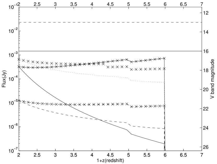
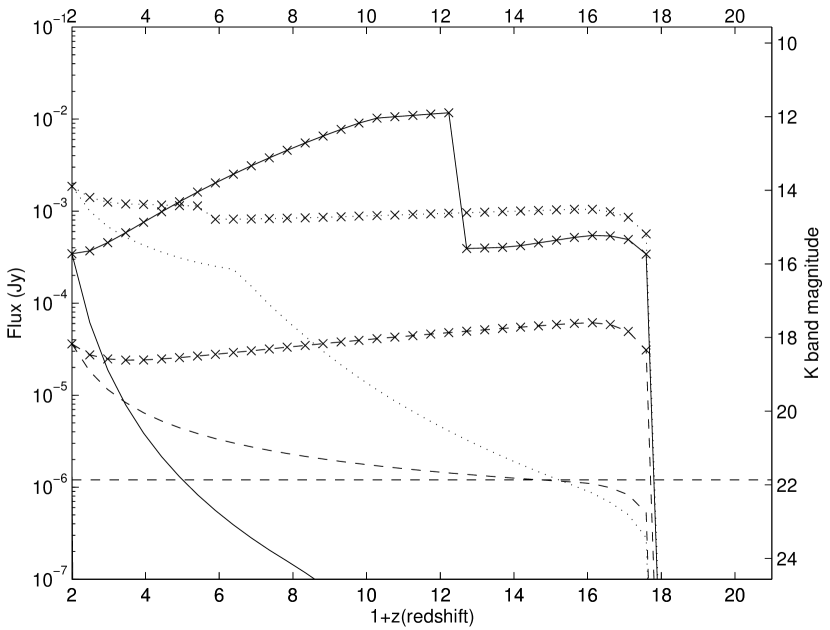
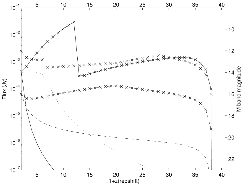
Figure 4: Combined forward and reverse shock observed flux as a function of redshift for the two density profiles $n=n_{0}=$ constant (without symbols) and $n=n_{0}(1+z)^{4}$ (symbols) with $n_{0}=0.01$ cm^-3. Solid, dashed and dotted lines indicate emission at different observer times t=10 mins, t=2 hour and t=1 day respectively. a): V-band ($\nu=5.45\times 10^{14}$ Hz); b): K-band ($\nu=1.36\times 10^{14}$ Hz); c): M-band ($\nu=6.3\times 10^{13}$ Hz). The limiting ROTSE and JWST sensitivities are the same as in Figure 2. Parameters: $\epsilon_{B,f}=0.001,{\cal R}_{B}=B_{r}/B_{f}=5,\epsilon_{e}=0.1,E_{52}=10,p=2.5,\eta=120.$

We further tested a different normalization, i.e. $n_{0}=0.01\ {\rm cm^{-3}}$, still for ${\cal R_{B}}=5$. The same total forward plus reverse shock flux for the two density profiles for this case are shown in Figure 4. An obvious feature is that the reverse shock is much more prominent for the lower normalization density ($n_{0}=0.01\ {\rm cm^{-3}}$) case than for the higher normalization density ($n_{0}=1\ {\rm cm^{-3}}$) case, in the density evolution model. From equations (A4, A5, A20 & A19), for slow cooling, the ratio of reverse shock to forward shock emission is proportional to $n^{(1/6-1/2)}=n^{-1/3}$ or $n^{(1/3-1/2)}=n^{-1/6}$. Therefore, the reverse shock emission becomes more prominent for a decreasing number density. However, we also note that the reverse shock emission is smaller than the forward shock flux in some cases. This is because the reverse shock is in the $\nu_{m,r}<\nu<\nu_{c,r}$ regime before the crossing time. So the ratio of the reverse shock to forward shock flux is proportional to $n^{(3p+1)/4}$. When the number density is smaller than 1 $\rm cm^{-3}$, we can expect the reverse shock flux to be smaller. The same is also expected for the constant density case at an early observer time. So in this case these two density models can be easily differentiated from each other.

3.3 X-ray Flux Redshift Dependence

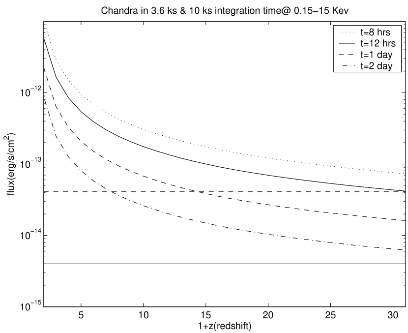
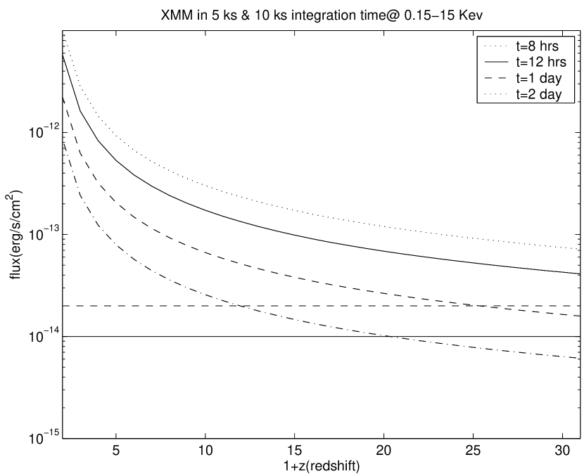
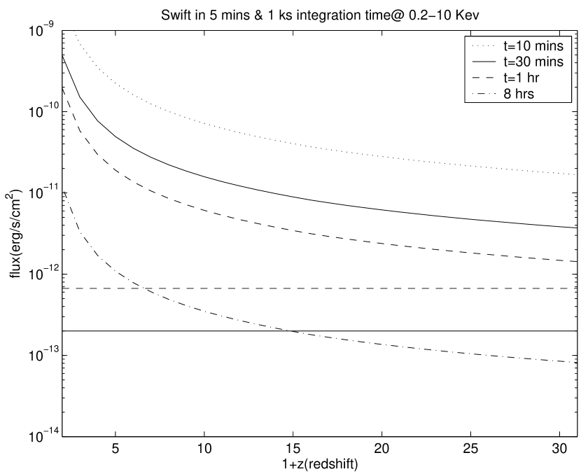
Figure 5: Observed X-ray fluxes for GRB afterglows at different redshifts, integrated over the observing energy ranges of 0.4-6 keV for Chandra, 0.15-15 Kev for XMM and 0.2-10 keV for Swift, respectively. The emission is in the density-independent regime, above $\nu_{c,f}$. a): for Chandra, the fluxes for the observer times $t_{obs}=$ 8 hour, 12 hours, 1 day and 2 days as compared to its sensitivities shown as horizontal lines for integration times of 3.6 ks (dashed) and 10 ks (solid). b): for XMM, same observer times as Chandra’s. The sensitivity horizontal lines are for integration times of 5 ks (dashed) and 10 ks (solid). c): for Swift XRT, the fluxes are for observer time $t_{obs}=$ 10 mins, 20 mins, 1 hour. The sensitivity horizontal lines are for integration times 300 s (dashed) and 1 ks (solid). Parameters: $\epsilon_{B,f}=0.001,{\cal R}_{B}=B_{r}/B_{f}=5,\epsilon_{e}=0.1,E_{52}=10,p=2.5,\eta=120.$

The X-ray band flux evolution and its redshift dependence is simpler than in the O/IR bands because the reverse shock emission is generally negligible, and we need only consider the forward shock emission. One obvious characteristic of Figure 5 is that the flux from the two different density profiles are the same at all the redshifts for a given time, because the emission in both cases is in the density-independent regime, being above the cooling frequency $\nu_{c,f}$. Based on equation (12), for an arbitrary choice of low X-ray energy of 0.1 keV and using the other parameters above, we obtain a critical redshift $z_{c}=0.83$ (n=const) or $z_{c}=0.98\ (n\propto(1+z)^{4})$ where the GRBs change from the density-dependent to the density-independent regime at an observer time $t=10$ mins. In addition, we know that $(1+z_{c})\propto t^{-1}\nu^{-2}$ based on eqn (12). As the observer time or observer’s frequency is increased, the critical redshift decreases, if the other parameters remain unchanged. Therefore, in the range of redshifts concerned, GRBs in these two different density profiles are always in the density-independent regime and the corresponding fluxes will always be same. On Figure 5 (a) and (b), the X-ray flux is calculated for observer times $t=8\ {\rm hours},\ 12\ {\rm hours},\ 1\ {\rm day}$ and $2\ {\rm days}$ for Chandra and XMM, respectively. The flux is integrated over the $0.4-6$ keV range of the Chandra ACIS instrument, and over 0.15-15 kev for XMM. Although it takes about 1 day or so for Chandra to slew onto the source, we see that Chandra is still able to detect GRBs with the typical parameters considered here up to $z\approx 30$ at 1 day with a 10 ks integration. XMM has proved itself capable of $\lesssim\ 8\ {\rm hours}$ slewing onto GRBs and has a similar sensitivity to Chandra, hence it might be able to detect higher redshift GRBs than Chandra does. In Figure 5(c), we have integrated the X-ray flux over the Swift XRT frequency range of $0.2-10$ keV. Although Swift XRF has a relatively lower sensitivity than Chandra and XMM, this is compensated by its quick slewing time, less than 1 minute. In Figure 5(c) we see that Swift XRT can easily detect typical GRBs up to redshifts $\sim 30$, if they are observed within 1 hour after the trigger. Therefore, if GRBs exist at very high redshift, we can expect these detectors to be able to measure them in x-ray band.

4 Summary and Conclusions

In this paper, we have calculated the spectral time evolution and the flux in the near-IR K- and M-bands as well as in the X-ray band from GRBs at very high redshifts and different times. In previous work, Ciardi & Loeb (2000) calculated IR fluxes as a function of redshift and time for the standard forward shock model of afterglows. Lamb & Reichart (2000) discussed the optical/IR as well as gamma-ray fluxes of some observed bursts at an observer time of 1 day when placed at different redshifts. Here we have introduced several new elements in our analysis, motivated by recent developments in the observations as well as in the modeling of bursts. The most important of these is that we consider, in addition to the forward shock, also the reverse shock, which has now been inferred in three GRBs from prompt follow-ups. The quick response capability of a number of ground and space observing facilities coming on-line in the near future means that one is far likelier to observe the early stages of the GRB and of its afterglow evolution. Thus there are excellent prospects for observing the reverse shock thought to be responsible for the prompt optical flashes, which is prominent only at early times in the burst evolution. The observation of reverse shocks will, in addition, provide significant independent information on early GRB evolution, such as the initial Lorenz factor, the strength of magnetic fields, etc. (e.g. Zhang et al. 2003). Another difference with previous flux calculations is that we have used significantly updated model parameters, based on new data acquired in the past two years. Thus, for instance, we make use of the emerging consensus view that $\epsilon_{B,f}$ is usually smaller than $\epsilon_{e,f}$. As is seen from the calculations presented here, the magnetic field equipartition value has a significant effect on the flux.

We have calculated the flux from high redshift GRBs taking typical parameters, which gives a sense for how far GRBs can be detected using current or forthcoming instruments. In reality, these parameters would vary over a wide range, which would also affect the detectability. Zhang et al. (2003) have reexamined the three cases of GRB 990123, GRB 021004 and GRB 021211 and found evidence for an enhancement of the magnetic field in the reverse shock over that in the forward shock, by as much as a factor of ${\cal R}_{B}=B_{r}/B_{f}\approx 15$ (GRB 990123), i.e. $\epsilon_{B}$ in reverse shock is much larger that in the forward shock. If so, based on eqns. (A12-A17), we can see that if $\cal R_{B}$ increases, the observed (optical/IR) flux for the reverse shock component increases significantly as illustrated by comparing Figures (2) and (3). Separately, it has recently been recognized that there are burst to burst variations in the total beaming-corrected energy, and thus, the forward shock peak afterglow fluxes may also be significant (Bloom, Frail, & Kulkarni 2003). The so-called ‘fGRBs’ exhibit rapid, jet-break like decays at early times, before the $\lesssim 1$ day point at which they would usually be expected. Thus we can expect that the reverse shocks in this kind of GRBs are less bright.

Most of the radiation in the optical and ultraviolet bands from high redshift extragalactic sources, including GRBs, is absorbed by the intergalactic medium and the diffuse gas in our own galaxy. The X-ray and infrared bands are therefore of major importance for detecting and tracking high-redshift GRBs. Several major ground-based telescopes as well as smaller robotic facilities have or will have infrared sensitivity in the K, L and M-bands. Next generation spacecraft such as Swift have X-ray and optical/UV detectors, while the James Webb Space Telescope (JWST) frequency range extends out to 27 $\mu$m, being most sensitive in the 1-5 $\mu$m J,H,K,L and M bands. In the X-ray band, the Chandra and XMM sensitivities in 0.2-10 keV are substantially higher than that of Swift XRT, but their slewing time ($\lesssim 1$ day) limitations make Swift XRT a unique instrument for X-ray follow-up during the first day after a GRB trigger, when the burst is brighter. In spite of this, all three spacecraft should be able to detect very distant GRBs, if they exist, e.g. at $z\gtrsim 30$.

For the nominal GRBs considered here, the luminosities are comparable to those of the currently detected ones. According to theoretical modeling, the fractional number of GRBs expected at $z\gtrsim 5$ is $\gtrsim 50\%$ of which $\sim 15\%$ may be detectable in flux-limited surveys such as Swift’s (Bromm & Loeb 2002). It was reported that HETE-2 sees 13 out of 14 GRB optical afterglows by Sep. 2003, which means that the high-$z$ GRB fraction is small (Ricker 2003). However, recently another high-z GRB candidate (GRB 031026) was detected and proposed (e.g. Atteia et al. 2003), which increases the high-$z$ fraction to be close to 15$\%$. We note also that at $z\gtrsim 6-10$ the first generation of (pop III) stars are likely to lead to black holes with masses $10-30~{}M_{\odot}$, and hence to GRBs whose luminosities could be factors 10-30 times higher (e.g. Mészáros & Rees 2003) than assumed here. In this case, the fraction at $z\gtrsim 5$ detectable in Swift’s flux-limited survey could be $\gtrsim 20-30\%$ of the total, or $\gtrsim 20$/year.

In the K and M bands (2.2 and 4.8 $\mu$m) the JWST and other telescopes should be able to detect afterglows out to $z\lesssim 16$ and 33 within observer times 1 day for integrations times (with JWST) of 1 hour (at a resolution R=1000 and S/N=10; see Figure 3 and Figure 4). These bands are accessible also to ground-based telescopes already on line, before the JWST launch. The effect of reverse shocks, which are brighter in the O/IR at early source times for some bursts, makes for a significantly increased sensitivity at high redshifts at observer times $\lesssim$ 1 day.

We have also considered the effect of two different types of the near-burst environment, one assuming that the external density evolves with redshift similarly to that in protogalactic disks, and the other assuming approximately redshift-independent conditions regulated by radiation pressure, based on primordial star formation calculations. The predicted X-ray fluxes, being due mainly to forward shocks above the cooling frequency, are independent of the external density regime, as well as insensitive to the existence of reverse shocks. However the IR fluxes are sensitive to which of these density regimes prevails, and at early times are very sensitive to the presence and strength of a reverse shock component, in particular at early times and redshifts $\lesssim 15$. Combining these two types of IR and X-ray flux information will thus provide very important tools for detecting GRBs (if present) out to very high redshifts, for studying their local environments, and for investigating the effects of reverse shocks as well as the prompt phases of the bursts and their afterglows.

Appendix A Appendix: Flux Evolution

A.1 Forward Shock

The radiation emitted by a source at a redshift z at frequency $\nu_{s}$ over a time $\delta t$ will be observed at z=0 at a frequency $\nu_{0}(z=0)=\nu_{s}/(1+z)$ over a time $\delta t_{0}(z=0)=(1+z)\delta t_{s}$. The luminosity distance for a flat universe $\Omega_{\Lambda}+\Omega_{M}=1$, $\Omega_{M}=0.27$ and Hubble constant $(H/100)\ km/s/Mpc=0.7h_{70}$ can be approximated, in units of $10^{28}$ cm, as $D_{28}(z)\approx 4.49(1+z)[1-1.115(1+z)^{-1/2}]$ (Pen 1999). Substituting this redshift dependence and eqn. (5) into equations (1) and (2), we have for the fast cooling case

$$F_{\nu}=\left\{\begin{array}[]{l@{\quad\quad}l}C_{1}\epsilon_{B,f}E_{52}^{7/6}t_{5}^{1/6}n^{5/6}\nu^{1/3}(1+z)^{-5/6}x^{-2}&\nu<\nu_{c,f}\\ C_{2}\epsilon_{B,f}^{-1/4}E_{52}^{3/4}t_{5}^{-1/4}\nu^{-1/2}(1+z)^{-5/4}x^{-2}&\nu_{c,f}<\nu\leq\nu_{m,f}\\ C_{3}\epsilon_{B,f}^{(p-2)/4}\epsilon_{e}^{(p-1)}E_{52}^{(p+2)/4}t_{5}^{-(3p-2)/4}\nu^{-p/2}(1+z)^{(p-6)/4}x^{-2}&\nu_{m,f}\leq\nu\\ \end{array}\right.$$ (A1)

For the slow cooling case, we have

$$F_{\nu}=\left\{\begin{array}[]{l@{\quad\quad}l}C_{4}\epsilon_{B,f}^{1/3}\epsilon_{e}^{-2/3}E_{52}^{5/6}t_{5}^{1/2}n^{1/2}\nu^{1/3}(1+z)^{-7/6}x^{-2}&\nu<\nu_{m,f}\\ C_{5}\epsilon_{B,f}^{(p+1)/4}\epsilon_{e}^{(p-1)}E_{52}^{(p+3)/4}t_{5}^{-3(p-1)/4}n^{1/2}\nu^{(1-p)/2}(1+z)^{(p-5)/4}x^{-2}&\nu_{m,f}\leq\nu<\nu_{c,f}\\ C_{3}\epsilon_{B,f}^{{(p-2)}/4}\epsilon_{e}^{(p-1)}E_{52}^{(p+2)/4}t_{5}^{-(3p-2)/4)}\nu^{-p/2}(1+z)^{(p-6)/4}x^{-2}&\nu_{c,f}\leq\nu\\ \end{array}\right.$$ (A2)

where $C_{1}$=0.402, $C_{2}=8.65\times 10^{9}$, $C_{3}=(8.6\times 10^{9})\times(4.6\times 10^{14})^{(p-1)/2}=8.5\times 10^{20}\ (p=2.5)$, $C_{4}=0.071$,and $C_{5}=5.5\times 10^{3}\times(4.58\times 10^{14})^{(p-1)/2}=5.4\times 10^{14}\ (p=2.5)$ and $x$ is defined as

$$x=[1-1.115(1+z)^{-1/2}].$$ (A3)

Here, $\epsilon_{B,f},\epsilon_{e},E_{52}$ have been assumed to be constant parameters, while others like $D_{28}(z)$ and $n$ may be redshift dependent in different cases. $\nu$ is the observed frequency. For simplicity, we present here the scaling relation for the flux with several parameters which may change with redshift. We substitute each of these quantities into the expressions above, and get the scaling relations with redshift for different cases.

Fast cooling case:

$$F_{\nu}\propto\left\{\begin{array}[]{l@{\quad\quad}l}n^{5/6}(1+z)^{-5/6}x^{-2}&\nu<\nu_{c,f}\\ n^{0}(1+z)^{-5/4}x^{-2}&\nu_{c,f}<\nu<\nu_{m,f}\\ n^{0}(1+z)^{(p-6)/4}x^{-2}&\nu_{m,f}<\nu\\ \end{array}\right.$$ (A4)

Slow cooling case:

$$F_{\nu}\propto\left\{\begin{array}[]{l@{\quad\quad}l}n^{1/2}(1+z)^{-7/6}x^{-2}&\nu<\nu_{m,f}\\ n^{1/2}(1+z)^{(p-5)/4}x^{-2}&\nu_{m,f}<\nu<\nu_{c,f}\\ n^{0}(1+z)^{(p-6)/4}x^{-2}&\nu_{c,f}<\nu\\ \end{array}\right.$$ (A5)

Substituting the redshift dependence of the number density into the relations above gives straightforwardly the scaling relations for the different density cases.

A.2 Reverse Shock

The scalings here are taken from Kobayashi (2000) and Zhang et al. (2003). Here the crossing time is defined as $t_{\times}=max(T,t_{dec})$, where $T$ is the burst duration and $t_{dec}$ is defined as $[(3E/4\pi\eta^{2}nm_{p}c^{2})^{1/3}/2\eta^{2}c](1+z)$ in the observer frame. Also, $\hat{\eta}={\rm min}(\eta,\eta_{c}^{2}/\eta)$, where $\eta$ is the initial Lorentz factor and $\eta_{c}$ is defined as the critical initial Lorentz factor $\eta_{c}=125E_{52}^{1/8}n^{-1/8}T_{2}^{-3/8}(\frac{1+z}{2})^{3/8}$ (Zhang et al 2003). For the thin shell case, one has $t_{\times}=t_{dec}$ and $\hat{\eta}=\eta$, while for the thick shell case, one has $t_{\times}=T$ and $\hat{\eta}=\eta_{c}^{2}/\eta$.

In the thick shell case, the typical parameters at crossing time $t_{\times}$ are:

$$\nu_{m,r}(t_{\times})=(\hat{\eta})^{-2}{\cal R_{B}}\nu_{m,f}(t_{\times}),\ \nu_{c,r}(t_{\times})={\cal R_{B}}^{-3}\nu_{c,f}(t_{\times}),\ F_{\nu,max,r}(t_{\times})=\hat{\eta}{\cal R_{B}}F_{\nu,max,f}(t_{\times})$$ (A6)

where ${\cal R_{B}}\equiv B_{r}/B_{f}=\left(\epsilon_{B,r}/\epsilon_{B,f}\right)^{1/2}$.

The scaling relations before and after the shock crossing time $t_{\times}$ are

$$t<t_{\times}:~{}~{}~{}\nu_{m,r}\propto t^{0},\\ \nu_{c,r}\propto t^{-1},\\ \ F_{\nu,m,r}\propto t^{1/2}$$ (A7)

$$t>t_{\times}:~{}~{}~{}\nu_{m,r}\propto t^{-73/48}\simeq t^{-3/2},\\ \nu_{c,r}\propto t^{-73/48}\simeq t^{-3/2},\\ \ F_{\nu,m,r}\propto t^{-47/48}\simeq t^{-1}$$ (A8)

For the thin shell case, at the crossing time, one has,

$$\nu_{m,r}(t_{\times})=\eta^{-2}{\cal R_{B}}\nu_{m,f}(t_{\times}),\ \nu_{c,r}(t_{\times})={\cal R_{B}}^{-3}\nu_{c,f}(t_{\times}),\ F_{\nu,m,r}(t_{\times})=\eta{\cal R_{B}}F_{\nu,m,f}(t_{\times})$$ (A9)

The scaling relations before and after the shock crossing time $t_{\times}$ are

$$t<t_{\times}:~{}~{}~{}\nu_{m,r}=t^{6},\\ \nu_{c,r}\propto t^{-2},\\ \ F_{\nu,m,r}\propto t^{3/2}$$ (A10)

$$t>t_{\times}:~{}~{}~{}\nu_{m,r}\propto t^{-54/35}\simeq t^{-3/2},\\ \nu_{c,r}\propto t^{-54/35}\simeq t^{-3/2},\\ \ F_{\nu,m,r}\propto t^{-34/35}\simeq t^{-1}$$ (A11)

Before the crossing time, for the thin shell case observed flux can be expressed as:

$$F_{\nu}=\left\{\begin{array}[]{l@{\quad\quad}l}[F_{\rm{\nu,f}}\nu_{\rm{c,f}}^{-1/3}\nu^{1/3}][\hat{\eta}{\cal R_{B}}^{2}(t/t_{\times})^{5/6}]&\nu<\nu_{c,r}\\ {[F_{\rm{\nu,f}}\nu_{\rm{c,f}}^{1/2}\nu^{-1/2}]}[\hat{\eta}{\cal R_{B}}^{-1/2}(t/t_{\times})^{1/2}]&\nu_{c,r}<\nu\leq\nu_{m,r}\\ {[F_{\rm{\nu,f}}\nu_{\rm{m,f}}^{(p-1)/2}\nu_{\rm{c,f}}^{1/2}\nu^{-p/2}]}[{\hat{\eta}}^{(2-p)}{\cal R_{B}}^{(p-2)/2}(t/t_{\times})^{(3p-5/2)}]&\nu_{m,r}\leq\nu\\ \end{array}\right.$$ (A12)

$$F_{\nu}=\left\{\begin{array}[]{l@{\quad\quad}l}[F_{\rm{\nu,f}}\nu_{\rm{m,f}}^{-1/3}\nu^{1/3}][{\hat{\eta}}^{(5/3)}{\cal R_{B}}^{2/3}(t/t_{\times})^{5/6}]&\nu<\nu_{m,r}\\ {[F_{\rm{\nu,f}}\nu_{\rm{m,f}}^{(p-1)/2}\nu^{-(p-1)/2}]}[{\hat{\eta}}^{(2-p)}{\cal R_{B}}^{(p+1)/2}(t/t_{\times})^{3p+3/2}]&\nu_{m,r}<\nu\leq\nu_{c,r}\\ {[F_{\rm{\nu,f}}\nu_{\rm{m,f}}^{(p-1)/2}\nu_{\rm{c,f}}^{1/2}\nu^{-p/2}]}[{\hat{\eta}}^{(2-p)}{\cal R_{B}}^{(p-2)/2}(t/t_{\times})^{(3p-5/2)}]&\nu_{c,r}\leq\nu\\ \end{array}\right.$$ (A13)

while for the thick shell the flux is:

$$F_{\nu}=\left\{\begin{array}[]{l@{\quad\quad}l}[F_{\rm{\nu,f}}\nu_{\rm{c,f}}^{-1/3}\nu^{1/3}][\hat{\eta}{\cal R_{B}}^{2}(t/t_{\times})^{5/6}]&\nu<\nu_{c,r}\\ {[F_{\rm{\nu,f}}\nu_{\rm{c,f}}^{1/2}\nu^{-1/2}]}[\hat{\eta}{\cal R_{B}}^{-1/2}]&\nu_{c,r}<\nu\leq\nu_{m,r}\\ {[F_{\rm{\nu,f}}\nu_{\rm{m,f}}^{(p-1)/2}\nu_{\rm{c,f}}^{1/2}\nu^{-p/2}]}[\hat{\eta}^{(2-p)}{\cal R_{B}}^{(p-2)/2}]&\nu_{m,r}\leq\nu\\ \end{array}\right.$$ (A14)

$$F_{\nu}=\left\{\begin{array}[]{l@{\quad\quad}l}[F_{\rm{\nu,f}}\nu_{\rm{m,f}}^{-1/3}\nu^{1/3}][\hat{\eta}^{(5/3)}{\cal R_{B}}^{2/3}(t/t_{\times})^{1/2}]&\nu<\nu_{m,r}\\ {[F_{\rm{\nu,f}}\nu_{\rm{m,f}}^{(p-1)/2}\nu^{-(p-1)/2}]}[\hat{\eta}^{(2-p)}{\cal R_{B}}^{(p+1)/2}(t/t_{\times})^{1/2}]&\nu_{m,r}<\nu\leq\nu_{c,r}\\ {[F_{\rm{\nu,f}}\nu_{\rm{m,f}}^{(p-1)/2}\nu_{\rm{c,f}}^{1/2}\nu^{-p/2}]}[\hat{\eta}^{(2-p)}{\cal R_{B}}^{(p-2)/2}]&\nu_{c,r}\leq\nu\\ \end{array}\right.$$ (A15)

After the crossing time, for both the thick shell and thin shell cases the expressions for the flux are:

$$F_{\nu}=\left\{\begin{array}[]{l@{\quad\quad}l}[F_{\rm{\nu,f}}\nu_{\rm{c,f}}^{-1/3}\nu^{1/3}][{\hat{\eta}}{\cal R_{B}}^{2}(t/t_{\times})^{-1/2}]&\nu<\nu_{c,r}\\ 0&\nu_{c,r}<\nu\leq\nu_{m,r}\\ 0&\nu_{m,r}\leq\nu\\ \end{array}\right.$$ (A16)

$$F_{\nu}=\left\{\begin{array}[]{l@{\quad\quad}l}[F_{\rm{\nu,f}}\nu_{\rm{m,f}}^{-1/3}\nu^{1/3}][{\hat{\eta}}^{5/3}{\cal R_{B}}^{3/2}(t/t_{\times})^{-1/2}]&\nu<\nu_{m,r}\\ {[F_{\rm{\nu,f}}\nu_{\rm{m,f}}^{(p-1)/2}\nu^{-(p-1)/2}]}[{\hat{\eta}}^{(2-p)}{\cal R_{B}}^{(p+1)/2}(t/t_{\times})^{(1-3p)/4}]&\nu_{m,r}<\nu\leq\nu_{c,r}\\ 0&\nu_{m,r}\leq\nu\\ \end{array}\right.$$ (A17)

Substituting the redshift dependence into equations above for the reverse shock, we obtain similar scaling relations as those for the forward shock.

For the thin shell case before crossing time:

Fast cooling case:

$$F_{\nu}\propto\left\{\begin{array}[]{l@{\quad\quad}l}n^{19/18}(1+z)^{-5/6}x^{-2}&\nu<\nu_{c,r}\\ n^{13/12}(1+z)^{-5/4}x^{-2}&\nu_{c,r}<\nu<\nu_{m,r}\\ n^{(5p-4)/4}(1+z)^{(p-6)/4}x^{-2}&\nu_{m,r}<\nu\\ \end{array}\right.$$ (A18)

Slow cooling case:

$$F_{\nu}\propto\left\{\begin{array}[]{l@{\quad\quad}l}n^{11/18}(1+z)^{-7/6}x^{-2}&\nu<\nu_{m,r}\\ n^{(3p+3)/4}(1+z)^{(p-5)/4}x^{-2}&\nu_{m,r}<\nu<\nu_{c,r}\\ n^{(5p-4)/4}(1+z)^{(p-6)/4}x^{-2}&\nu_{c,r}<\nu\\ \end{array}\right.$$ (A19)

For the thin shell case after the crossing time:

Fast cooling case:

$$F_{\nu}\propto\left\{\begin{array}[]{l@{\quad\quad}l}n^{11/18}(1+z)^{-5/6}x^{-2}&\nu<\nu_{c,r}\\ 0&\nu_{c,r}<\nu<\nu_{m,r}\\ 0&\nu_{m,r}<\nu\\ \end{array}\right.$$ (A20)

Slow cooling case:

$$F_{\nu}\propto\left\{\begin{array}[]{l@{\quad\quad}l}n^{1/6}(1+z)^{-7/6}x^{-2}&\nu<\nu_{m,r}\\ n^{1/3}(1+z)^{(p-5)/4}x^{-2}&\nu_{m,r}<\nu<\nu_{c,r}\\ 0&\nu_{c,r}<\nu\\ \end{array}\right.$$ (A21)

One sees that if the number density around the GRBs does not change with the redshift, i.e. $n=$ constant for all $z$, the reverse shock emission depends on redshift in the same way as the forward shock emission. However, in the $n\propto(1+z)^{4}$ case, the behavior for the reverse and forward shock emission is different. The thick shell behavior can be obtained in a similar way.

References

- (1) Abel,T., Anninos, P., Norman, M. L., & Zhang, Y. 1998, ApJ, 508, 518
- (2) Abel T., Bryan G.L, & Norman M.L. 2000, ApJ, 540, 39
- (3) Abel, T., Bryan, G.L., & Norman, M.L. 2002, Science, 295, 93
- (4) Akerlof, C.W. et al. 1999, Nature, 398, 400
- (5) Atteia, J.L. et al. 2003, GCN #2432
- (6) Barkana, R., & Loeb, A. 2000, ApJ, 531, 613
- (7) Barkana, R., & Loeb, A. 2001, Physics Reports, 349, 125
- (8) Bennett, C.L., Halpern, M., Hinshaw, G., et al. 2003, ApJS, 148, 1
- (9) Bloom, J.S., Frail, D.A.,& Kulkarni, S.R. 2003, ApJ, 594, 674
- (10) Bromm, V., Coppi, P.S., & Larson, R.B. 1999, ApJ, 527, L5
- (11) Bromm, V., & Loeb, A. 2002, ApJ, 575, 111
- (12) Ciardi, B., & Loeb, A. 2000, ApJ, 540, 687
- (13) Chevalier, R., & Li, Z.Y. 1999, ApJ, 520,L29
- (14) Dai, Z.G., & Lu, T. 1998, MNRAS, 298, 87
- (15) Fan X.H., et al. 2001, AJ, 121, 54
- (16) Fan X.H., et al. 2003, AJ, 125, 1649
- (17) Fenimore, E.E., & Ramirez-Ruiz,. E. 2000, astro-ph/0004176
- (18) Fox, D.W. et al. 2003a, Nature, 422, 284
- (19) Fox, D.W. et al. 2003b, ApJ, 586, L5
- (20) Frail, D.A. et al. 2001, ApJ, 562, L55
- (21) Lamb, D.Q., & Reichart, D.E. 2000, ApJ, 536, 1
- (22) Li, W.D. et al. 2003, ApJ, 586, L9
- (23) Haiman, Z., & Loeb, A. 1997, ApJ, 483, 21
- (24) Hjorth, J, et al. 2003, Nature, 423, 847
- (25) Kauffmann, G., White, S.D.M., & Guiderdoni, B. 1993, MNRAS, 264, 201
- (26) Kobayashi, S. 2000, ApJ, 545, 807
- (27) Kobayashi, S., & Zhang, B. 2003, ApJ, 582, L75
- (28) Madau, P., Haardt, F., & Rees, M.J. 1999, ApJ, 514, 648
- (29) Mészáros, & Rees, M. 2003, ApJ, 591, L91-L94
- (30) Mészáros, & Rees, M., & Wijers, R.A.M.J. 1998, ApJ, 499, 301
- (31) Miralda-Escudé, J. 1998, ApJ, 501, 15
- (32) Miralda-Escudé, J. 2001, ApJ, 528, L1
- (33) Miralda-Escudé, J. 2003, Science, 300, 1904
- (34) Mo, H.J., Mao, S.D., & White, S.D.M. 1998, MNRAS, 295, 319
- (35) Norris, J.P., Marani, G., & Bonnel, J. 2000, ApJ, 534, 248
- (36) Morrison, R., & McCammon, D. 1983, ApJ, 270, 119
- (37) Onken, P., & Miralda-Escudé, J. 2003, ApJ, submitted (astro-ph/037184)
- (38) Padmanadhan, T. 2001, Theoretical Astrophysics, v1, p25 (Cambridge University Press)
- (39) Panaitescu, A., & Kumar, P. 2001, ApJ, 560, 49
- (40) Panaitescu, A., & Kumar, P. 2002, ApJ, 571, 779
- (41) Pen, U.L. 1999, A&ASS, 120, 49
- (42) Perna, R., & Loeb, A. 1998, ApJ, 501, 467
- (43) Price P.A., et al. 2003, Nature, 423, 844
- (44) Ricker G. 2003 GRB conference, Santa Fe
- (45) Sari, R., Piran,T., & Narayan, R. 1998 ApJ, 497, L17
- (46) Spergel, D. N., et al. 2003, ApJS, 148, 175
- (47) Stanek, K., et al. 2003, ApJ, 591, L17
- (48) Uemura M., et al. 2003, Nature, 423, 843
- (49) van Paradijs, J., Kouveliotou, C., & Wijers, R.A.M. J. 2000, ARA&A, 38, 379
- (50) Whalen, D., Abel, T., & Norman, M. L. 2003, ApJ, submitted (astro-ph/0310284)
- (51) Zhang, B., Kobayashi, S., & Mészáros, P. 2003, ApJ, 595, 950