Broad redshifted line as a signature of outflow

Abstract

We formulate and solve the diffusion problem of line photon propagation in a bulk outflow from a compact object (black hole or neutron star) using a generic assumption regarding the distribution of line photons within the outflow. Thomson scattering of the line photons within the expanding flow leads to a decrease of their energy which is of first order in $v/c$, where $v$ is the outflow velocity and $c$ is the speed of light. We demonstrate that the emergent line profile is closely related to the time distribution of photons diffusing through the flow (the light curve) and consists of a broad redshifted feature. We analyzed the line profiles for the general case of outflow density distribution. We emphasize that the redshifted lines are intrinsic properties of the powerful outflow that are supposed to be in many compact objects.

1 Introduction

The problem of photon propagation in an optically thick fluid in bulk motion has been studied in detail in a number of papers. The idea that photons may change their energy in repeated scatterings with cold electrons in a moving fluid was suggested more than 20 years ago by Payne & Blandford (1981), hereafter PB81 and Cowsik & Lee (1982). This process, often referred to as dynamical or bulk flow Comptonization, is similar in many ways to Comptonization by hot electrons once the thermal velocity is replaced by bulk velocity $\bf v$; there is however a qualitative difference, in that their energy gain is linear in the velocity $v$, rather than quadratic as is in the case of Compton scattering in a medium at rest. Photons diffusing and scattering in a medium with bulk flow can gain or lose energy to the flow depending on the divergence of its velocity field: they gain energy for $\nabla\cdot{\bf v}<0$, while they lose energy in the opposite case. The case of a converging radial inflow, where $\nabla\cdot{\bf v}<0$, has been treated by (among others) PB81, Nobili, Turolla, & Zampieri 1993, Turolla et al. (1996) and Titarchuk, Mastichiadis & Kylafis (1996; 1997), (hereafter TMK96, TMK97 respectively). These investigations showed that, when monochromatic radiation with $\nu=\nu_{*}$ is injected at large Thomson depth in a spherical inflow, the emergent spectrum develops a broad, power-law tail at $\nu>\nu_{*}$. The power law index is related to a combination of the flow Thomson depth and its velocity gradient, and this has been invoked to explain the high energy spectra of accreting BH candidate sources in their “high” state (Laurent & Titarchuk 1999; Shrader & Titarchuk 1999).

In this Paper we treat the problem of an outflow and show that a similar broad spectrum is formed but now at energies $\nu<\nu_{*}$, with the power law index dependent on the velocity gradient. This problem is also relevant observationally because of the well known presence of red wings in the fluorescent Fe K$\alpha$ line profiles observed in the AGN and galactic BH spectra. Turolla et al. (1996) were first who analyzed the radiative transfer in an expanding atmosphere. They found a particular solution of the PB81 equation for diverging flow using Fourier transformation. They showed that the overall behavior of the spectra is similar to that of the converging flow but somehow reversed, since now photons can drift only to frequencies lower than $\nu_{*}$. Furthermore, they found that adiabatic expansion produces a drift of injected monochromatic photons towards lower frequencies and the formation of a power-law, low energy tail with spectral index 3.

Photons can also lose energy in scattering with cold electrons due to recoil. This process was treated by Sunyaev & Titarchuk (1980; hereafter ST80), who demonstrated that the emergent spectrum of the high energy photons injected in the static cold electron cloud is determined by the initial photon distribution in radius, which in turn dictates the photon escape probability distribution in time. The resulting spectrum for monochromatic injection is a redshifted feature of spectral width $\Delta\nu$ which depends on the line frequency $\nu_{*}$ and the Thomson depth $\tau_{0}$, i.e. $\Delta\nu\sim-\nu_{*}(h\nu_{*}/m_{e}c^{2})\tau_{0}^{2}$. The observation of red-skewed K${\alpha}-$lines observed in a number of AGN (and galactic black hole systems) (Fabian et al. 1995), led to the consideration of the role of this process in producing the observed Fe line profiles. This was however dismissed by Fabian et al. (1995), who correctly pointed out that the required Thomson downscattering of the line photons would also introduce a (non-observed) break in the spectrum at energy $E\simeq m_{e}c^{2}/\tau_{0}^{2}\simeq 20$ keV. An approach along the same lines by Misra & Kembhavi (1998) was rebutted on the basis of line and continuum variability observations by Reynolds & Wilms (2000).

Following these works, the prevailing process for producing the observed profile of the Fe K$\alpha-$line was considered to be Doppler broadening by the kinematics of a cold ($kT<0.25$ keV) accretion disk reprocessing the X-ray radiation of an overlying corona into fluorescent Fe K$\alpha-$line and reflection continuum. It was shown (Fabian et al. 1989) that such an arrangment could produce lines of the desired width and asymmetry provided that the disk extended to its innermost stable orbit (3 Schwarzschild radii). However plausible, this interpretation is not entirely without problems; for instance, the (occasionaly) exceedingly broad red wing of the line observed requires (in such cases) that the disk illumination be concentrated very close to its inner edge ($F_{x}\propto r^{-8}$; Nandra et al. 1999) more than most models would allow; this led Reynolds & Begelman (1997) to consider fluorescent emission from within the innermost stable orbit, by matter inspiraling into the black hole. Also, as indicated by the models of Nayakshin et al. (2000); Ballantyne et al. (2001), the ionization of such a disk by the intense X-ray radiation might invalidate some of basic assumptions associated with this interpretation. Of additional interest is also the fact that there is a marked absence of a blue-shifted wing in the line, a feature expected for a random orientation of accretion disks and the observers’ lines of sight.

Motivated by the above facts and the importance of the Fe K$\alpha-$line in probing the strong field limit gravity we believe it is important that all potential alternatives to line broadening be considered in detail. To this end we examine in the present Paper under what conditions these broad Fe line profiles could be also attributed to the effects of an outflow rather than solely to accretion disk kinematics. The formulation of the photon diffusion problem in an outflow and its solutions are described in §2, and in §3 our results are discussed and certain conclusions are drawn.

2 Radiative Transfer in a Bulk Outflow

2.1 Main equations and parameters

Let $N(r)=N_{0}(r_{0}/r)^{\beta}$ be the radial number density profile of an outflow and let its radial outward speed be

$$v_{b}/c=(\dot{M}_{out}/4\pi cN_{0}r_{0}^{2})(r_{0}/r)^{2-\beta}=\dot{m}_{out}(r_{0}/r)^{2-\beta}$$ (1)

obtained from mass conservation in a spherical geometry (here $\dot{M}_{out}=4\pi r^{2}v_{b}N$). The Thomson optical depth of the flow from some radius r to infinity is given by

$$\tau=\int_{r}^{\infty}N_{e}(r)\sigma_{\rm T}~{}dr=\sigma_{\rm T}N_{0}r_{0}(r_{0}/r)^{\beta-1}/(\beta-1),$$ (2)

where $N_{e}(r)=N(r)$ is the electron density, $\sigma_{\rm T}$ is the Thomson cross section, $r_{0}$ is a radius at the base of the outflow (this definition of optical depth makes the tacit assumption that $\beta>1$) and $\tau_{T,0}=\tau(r_{0})=\sigma_{\rm T}N_{0}r_{0}/(\beta-1)$.

The transfer of radiation within the flow in space and energy is governed by the photon kinetic equation (BP81, Eq. 18) for the photon occupation number $n(r,\nu)$, which in steady state reads

$$-{\bf v_{b}}\cdot\nabla n+\frac{1}{3}\nabla\cdot(\frac{c}{\kappa}\nabla n)+\frac{1}{3}(\nabla\cdot{\bf v_{b}})\,\nu\frac{\partial n}{\partial\nu}=-{\tilde{j}}(r,\nu),$$ (3)

where $\kappa=N_{e}(r)\sigma_{\rm T}$ is the inverse of the scattering mean free path, ${\bf v_{b}}=v_{b}{\bf e_{r}}$, is the flow velocity, ${\bf e_{r}}$ is the radial unit vector and $\tilde{j}(r,\nu)$ is the photon source term.

The spectral flux $F(r,\nu)$ (PB81) is given in terms of $n(r,\nu)$ by

$$F(r,\nu)=-\frac{1}{3\kappa(r)}\nabla n-\frac{1}{3}v_{b}\,\nu\frac{\partial n}{\partial\nu},$$ (4)

and must satisfy the following boundary conditions: (a) Conservation of the frequency integrated flux over the outer boundary, namely

$$\int F(r,\nu)d\nu\propto r^{-2}~{}~{}~{}{\rm as}~{}~{}{\rm r\rightarrow\infty}.$$ (5)

(b) The occupation number should be zero at the inner boundary $r=r_{0}$, where the bulk outflow starts and the outflow radiation is zero, i.e.

$$n(r_{0})=0.$$ (6)

2.2 Solution for a general case of any optical depth $\tau_{0}$

According to a theorem (Titarchuk 1994, appendix A), the solution of any equation whose LHS operator acting on the unknown function $n(r,\nu)$ is the sum of two operators $L_{r}$ and $L_{\nu}$, which depend correspondingly only on space and energy and the RHS, $j(r,\nu)$, is factorizable, i.e.

$$L_{r}n+L_{\nu}n=-j(r,\nu)=-f(r)\varphi(\nu)$$ (7)

with boundary conditions independent of the energy $\nu$, i.e.

$$L^{(1)}_{r}n=0~{}~{}~{}~{}{\rm as}~{}~{}{\rm r\rightarrow\infty},~{}~{}~{}~{}L^{(2)}_{r}n=0~{}~{}~{}~{}{\rm for}~{}~{}{\rm r=r_{0}}~{},$$ (8)

is given by the convolution of the solutions of the time-dependent problem of each operator, namely

$$n(r,\nu)=\int_{0}^{\infty}P(r,u)X(\nu,u)du.$$ (9)

Above $u=N_{0}\sigma_{\rm T}ct$ is the dimensionless time and $P(r,u)$ is the solution of the initial value problem of the spatial operator $L_{r}$

$$\frac{\partial P}{\partial u}=L_{r}P,~{}~{}~{}~{}~{}P(r,0)=f(r)$$ (10)

with boundary conditions

$$L^{(1)}_{r}P=0~{}~{}~{}~{}{\rm as}~{}~{}{\rm r\rightarrow\infty},~{}~{}~{}~{}L^{(2)}_{r}P=0~{}~{}~{}~{}{\rm at}~{}~{}{\rm r=r_{0}},$$ (11)

and $X(\nu,u)$ the solution of the initial value problem of the energy operator $L_{\nu}$

$$\frac{\partial X}{\partial u}=L_{\nu}X,~{}~{}~{}~{}~{}X(\nu,0)=\varphi(\nu)$$ (12)

with boundary conditions

$$\nu^{3}X\rightarrow 0~{}~{}~{}~{}{\rm when}~{}~{}~{}\nu\rightarrow 0,~{}\infty.$$ (13)

In the case where the photon energy change is due to the electron recoil (see details in ST80), we have

$$L_{r}n=\frac{1}{3\kappa}\nabla\cdot\left[\frac{1}{\kappa}\nabla n\right]$$ (14)

and

$$L_{\nu}n=\frac{1}{z^{2}}\frac{\partial}{\partial z}(z^{4}n).$$ (15)

where $z=h\nu/m_{e}c^{2}$. The solution of the time-dependent problem for the energy operator $L_{\nu}$ (the Green’s function) and $\varphi(z)=\delta(z-z_{\ast})/z^{3}$ is (see ST80)

$$J(z,u)=z^{3}X(z,u)=\left\{\begin{array}[]{ll}\delta[(1/z-u)^{-1}-z_{\ast}]/z&\mbox{if $z\leq z_{\ast}~{}{\rm and}~{}0\leq u\leq 1/z$}\\ 0&\mbox{otherwise,}\end{array}\right.\$$ (16)

where $J(z,u)=z^{3}X(z,u)$ is the radiation intensity. Substitution of Eq.(16) into Eq.(9) gives the form of the response function (the Green’s function) to monochromatic line injection in a static cloud

$$G_{z_{\ast}}(z)=z^{3}n(r_{out},z)=\frac{1}{z_{\ast}z}P[r_{out},(1/z-1/z_{\ast})].$$ (17)

For a local photon injection the time-dependent diffusion distribution in a bounded medium has the form of a fast rise and exponential decay (see ST80 and Wood et al. 2001), where the characteristic dimensionless time ($u=\sigma_{\rm T}N_{0}ct$) for the exponential decay is always proportional to $\tau_{\rm T,0}^{2}$, independent of the source distribution. Thus the asymptotic form of the redshifted wing of the downscattering line (i.e. for $\nu\ll\nu_{*}$) is always exponential, $G_{z_{\ast}}(z)\propto z^{-1}\exp(-A_{0}/z\tau_{\rm T,0}^{2})$. It is evident from this formula that a significant line redshift can occur only when $h\nu/m_{e}c^{2}\tau_{\rm T,0}^{2}\sim A_{0}$ where $A_{0}$ is of order of a few.

To obtain the Green’s function of the same problem for a diverging flow we use the same method applied in the downscattering case. The time-dependent problem for the energy Green’s function is (see Eq.3 and Eqs. 12-13)

$$\frac{\partial X}{\partial u}=L_{\nu}X=\nu\frac{\partial X}{\partial\nu}$$ (18)

$$X(\nu,0)=\delta(\nu-\nu_{\ast})/\nu^{3}$$ (19)

with boundary conditions

$$\nu^{3}X\rightarrow 0~{}~{}~{}~{}{\rm when}~{}~{}~{}\nu\rightarrow 0,~{}\infty.$$ (20)

The problem (18-20) is an initial value problem for the first order partial differential equation and it can be found using the method of characteristics (see e.g. Zel’dovich & Raizer, 2002) Because the occupation number $X(\nu,0)$ is conserved along the characteristics $u=\ln\nu_{0}/\nu$ of equation (18) the solution of the problem (18-20) is

$$J_{\nu_{\ast}}(\nu,u)=\nu^{3}X(\nu,u)=e^{-3u}\delta(\nu e^{u}-\nu_{\ast}).$$ (21)

Substitution of $J_{\nu_{\ast}}(\nu,u)$ from Eq.(21) into Eq.(9) gives us the Green’s function

$$G_{\nu_{\ast}}(\nu)=\nu^{3}n(r_{out},\nu)=\frac{1}{\nu_{\ast}}\left(\frac{\nu}{\nu_{\ast}}\right)^{3}P[r_{out},\ln(\nu_{\ast}/\nu)].$$ (22)

The time distrubition $P(r_{out},u)$ can be found from the solution of the time-dependent problem of the space operator and initial condition (see Eq. 10)

$$\frac{\partial P}{\partial u}=L_{r}P=\frac{\nabla\cdot[(1/\kappa)\nabla P]}{\nabla\cdot({\bf v_{b}}/c)}-3\frac{({\bf v_{b}}/c)\cdot\nabla P}{\nabla\cdot({\bf v_{b}}/c)},$$ (23)

$$P(r,0)=f(r)$$ (24)

with two boundary conditions

$$-(1/\kappa)\nabla P\propto r^{-2}~{}~{}~{}~{}{\rm at}~{}~{}{\rm r\rightarrow\infty},~{}~{}~{}~{}P=0~{}~{}~{}~{}{\rm at}~{}~{}{\rm r=r_{0}}.$$ (25)

Introducing $\tau=\tau_{\rm T}$ as a spatial variable Eq.(23) can be rewritten as follows

$$\frac{\partial P}{\partial u}=L_{r}P=\frac{\beta-1}{\beta}\left\{C_{v_{b}}^{-1}\tau^{\gamma}\left[\frac{\partial^{2}P}{\partial\tau^{2}}-\frac{2}{(\beta-1)\tau}\frac{\partial P}{\partial\tau}\right]+3\tau\frac{\partial P}{\partial\tau}\right\},$$ (26)

where $C_{v_{b}}=(\dot{M}_{out}/4\pi cN_{0}r_{0}^{2})\tau_{0}^{(\beta-2)/(\beta-1)}=\dot{m}_{out}\tau_{0}^{(\beta-2)/(\beta-1)}$, $\gamma=(2\beta-3)/(\beta-1)$. In order to solve the above time-dependent problem we look for solution of the eigenvalue problem for the operator $L_{r}$ (Eq. 26) with the appropriate boundary conditions, namely

$$L_{r}R+\lambda^{2}R=0,$$ (27)

with the boundary conditions

$$dR/d\tau\propto\tau^{2/(\beta-1)}\propto r^{-2}~{}~{}{\rm as}~{}~{}{\tau\rightarrow 0}~{}~{}({\rm or}~{}~{}r\rightarrow\infty)~{}~{}~{}{\rm and}~{}~{}~{}R=0~{}~{}{\rm at}~{}~{}{\rm\tau=\tau_{0}}.$$ (28)

The nontrivial solution of equation (27) satisfying the boundary conditions (28) (i.e. eigenfuction) is

$$R_{\lambda}(\tau)=\tau^{(\beta+1)/(\beta-1)}\Phi[\beta+1+\lambda^{2}\beta/3,\beta+2,-3C_{v_{b}}(\beta-1)\tau^{1/(\beta-1)}],$$ (29)

where $\Phi(a,b,z)$ is the confluent (or degenerate) hypergeometric function. The boundary conditions (28), along with formula (29), implies that the eigenvalues are roots of the equation

$$\Phi(\beta+1+\lambda^{2}\beta/3,\beta+2,-\tau_{eff,0})=0,$$ (30)

where $\tau_{eff,0}=3\dot{m}_{out}(\beta-1)\tau_{0}$. Using the asymptotic form of the confluent hypergeometric function $\Phi(a,b,z)$ for large arguments $z\gg 1$ (Abramowitz & Stegun 1970, Eq.[13.1.4])

$$\Phi(a,b,z)=\frac{\Gamma(b)}{\Gamma(b-a)}(-z)^{-a}[1+O(|z|^{-1})]$$ (31)

and equation (30) we can find the eigenvalues for $\tau_{eff,0}=3(\beta-1)\dot{m}_{out}\tau_{0}\gg 1$ as roots of the following equation

$$1/\Gamma(1-\lambda^{2}\beta/3)=0,$$ (32)

where $\Gamma(z)$ is the gamma-function. Because $\Gamma(z)$ goes to $\infty$ for nonpositive integers, $z=-(k-1)$, ($k=1,$ 2, 3,…), the eigenvalues are

$$\lambda_{k}^{2}=3k/\beta.$$ (33)

If the monochromatic line sources are distributed according to the eigenfunction $f(r)=R_{k}(\tau)$ then $P(\tau,u)$ is

$$P_{k}(\tau,u)=R_{k}(\tau)\exp(-\lambda_{k}^{2}u).$$ (34)

Thus when $f(r)\propto R_{k}(\tau)$ the Green’s function $G_{\nu_{\ast}}(\nu)$ [see formula (22)] is a power law

$$G_{\nu_{\ast}}(\nu)\propto\frac{1}{\nu_{\ast}}\left(\frac{\nu}{\nu_{\ast}}\right)^{3+\lambda_{k}^{2}}.$$ (35)

For $\tau_{eff,0}\gg 1$ the spectral index

$$\alpha_{k}=3+\lambda_{k}^{2}=3(1+k/\beta)$$ (36)

and the least spectral index $\alpha=\alpha_{1}=3(1+1/\beta)$. In Figure 1 we present numerical calculations of the least photon index $\Gamma=\alpha-1$ using Eq.(30) for various values of $\beta$ and $\tau_{eff,0}$. As it is seen from this figure $\Gamma-$values converge to the asymptotic values $\Gamma_{as}=2+3/\beta$ for $\tau_{eff,0}\gg 1$.

In the general case of a given source distribution $f(r)$, $m_{out}$, $\tau_{0}$, and $\beta$ one should calculate the eigenvalues using Eq. (30) and the expansion coefficients $b_{k}$ using the following formulae

$$b_{k}=\int_{0}^{\tau_{0}}\psi(\tau)R_{k}(\tau)f(\tau)d\tau/H_{k}(\tau_{0}),$$ (37)

$$H_{k}=\int_{0}^{\tau_{0}}\psi(\tau)R_{k}^{2}(\tau)d\tau,$$ (38)

where $\psi(\tau)=\tau^{(1-2\beta)/(\beta-1)}\exp(\xi)$ is a weight function, $\xi=3C_{v_{b}}(\beta-1)\tau^{1/(\beta-1)}$ is inversely proportional to the radius $r$ (see Eq. 2) and $C_{v_{b}}=\dot{m}_{out}\tau_{0}^{(\beta-2)/(\beta-1)}$. It is worth noting that the variable $\xi$ is equal to the trapping radius for advection, $r_{t}$, divided by the radius $r$, where $r_{t}=(GM/c^{2})(\dot{M}_{out}/\dot{M}_{E})$, with $\dot{M}_{E}=4\pi GMm_{H}/c\sigma_{T}$ denoting the Eddington accretion rate (see e.g. Becker & Begelman 1986, TMK97).

Equations (37-38) are obtained using the orthogonality properties of the eigenfunctions $R_{k}(\tau)$. In appendix A we show that the square norm $H_{k}$ can be computed analytically in closed form, namely that

$$H_{k}=p(\tau_{0})\frac{\partial R(\lambda_{k}^{2},\tau_{0})}{\partial(\lambda^{2})}\frac{\partial R_{k}(\tau_{0})}{\partial\tau},$$ (39)

where $p(\tau)=[(\beta-1)/\beta C_{v_{b}}]\tau^{\gamma}\psi(\tau)$ [see definition of $\gamma$ in Eq. (26) above]. Convenient formulae for calculations of derivatives of $R_{k}$ above are given in Appendix A. The numerator of equation (37) $c_{k}$ [a scalar product of $f(\tau)$ and $R_{k}(\tau)$] can be also calculated analytically in the case of the $\delta-$function source distribution [$f(\tau)=\delta(\tau-\tau_{\ast})$, where $\tau_{\ast}<\tau_{0}$]: $c_{k}=\psi(\tau_{\ast})R_{k}(\tau_{\ast})$.

The formula for the flux ${\cal F}(\nu)=[(r/r_{0})^{2}F(r,\nu)]|_{r\rightarrow\infty}$ (see Eq. 4) is

$${\cal F}(\nu)=[\tau^{2/(1-\beta)}F(\tau,\nu)]|_{\tau\rightarrow 0}\propto\frac{1}{\nu_{\ast}}\left(\frac{\nu}{\nu_{\ast}}\right)^{3}\sum_{k=1}^{\infty}b_{k}\left(\frac{\nu}{\nu_{\ast}}\right)^{\lambda_{k}^{2}}.$$ (40)

In order to calculate $R_{k}$ for $k\gg 1$ in equations (29, 37-38) one should use the asymptotic form of the confluent functions $\Phi(a,b,z)$ for large values of $a$ and $z>1$ (Abramowitz & Stegun 1970, Eq.[13.5.13]).

$$\Phi(a,b,z)=\Gamma(b)e^{z}(Z/4)^{(1/4-b/2)}\pi^{-1/2}\cos{(Z^{1/2}-b\pi/2+\pi/4),}$$ (41)

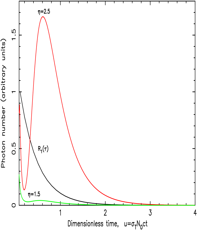
Figure 2: Plot of ${\cal P}(u)$ {${\cal P}(u)\propto[\tau^{2/(1-\beta)}\partial P/\partial\tau[\tau,u]|_{\tau\rightarrow 0}$} for three monochromatic source distributions: $f(\tau)=\exp{(\eta\xi)}$, for $\eta=1.5,~{}2.5$ and distributed according to the first eigenfunction $R_{1}(\tau)$ (see text). Plot for $\eta=0$ is not displayed here, because it is concentrated very close to $u=0$ in the presented scale. Calculations are made for $\beta=2$, $\dot{m}_{out}=0.8$ and $\tau_{0}=2$.

where $Z=(4a-2b)(-z)$. In Figure 2 we present the results of calculation of the time distribution ${\cal P}(u)\propto[\tau^{2/(1-\beta)}\partial P/\partial\tau[\tau,u]|_{\tau\rightarrow 0}$ using the expression [see Eq. (34) for the definition of $P_{k}(\tau,u)$]

$$P(\tau,u)=\sum_{k=1}^{\infty}b_{k}P_{k}(\tau,u)$$ (42)

and equations (29-30, 37-38). These particular calculations are made for a constant velocity wind ($\beta=2$), $\dot{m}_{out}=0.8$ and $\tau_{0}=2$, using as initial conditions a monochromatic source [$\varphi(\nu)=\delta(\nu-\nu_{\ast})$] and four different spatial distributions given by $f(\tau)=\exp{(\eta\xi)}$, with $\eta=0,~{}1.5,~{}2.5$ (i.e. sources increasingly concentrated towards the base of the flow for increasing $\eta$) and $f(\tau)=R_{1}(\tau)$, i.e. a distribution according to the first eigenfunction.

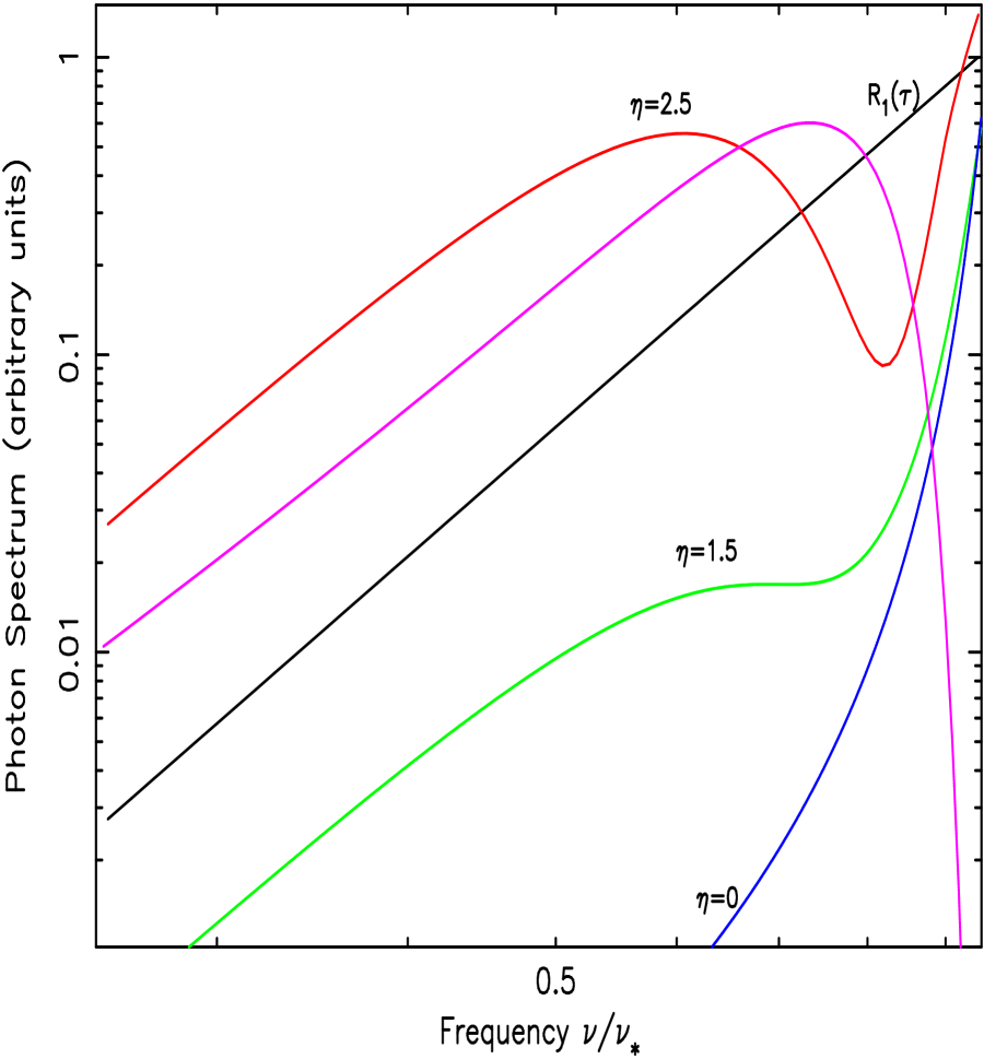
Figure 3: Plot of emergent photon redshifted line spectra. There are four spectra for monochromatic source distributions. $f(\tau)=\exp{(\eta\xi)}$, for $\eta=0,~{}1.5,~{}2.5$ and distributed according to the first eigenfunction $R_{1}(\tau)$ (see text). All these four spectra are related to ${\cal P}(u)$ through transformation (22) (see text). Calculations are made for $\beta=2$, $\dot{m}_{out}=0.8$ and $\tau_{0}=2$. The fifth photon spectrum (magenta) is for the asymptotic case of $\tau_{0}\gg 1$ (see formula 50). The monochromatic $\delta-$ function source is located at $\xi=\xi_{*}=2$, and $\beta=2$.

All spectra are related to $P(\tau,u)$ through the transformation of Eq. (22). In Figure 3 we show the evolution of the emergent spectra as a function of the initial source distribution $f(\tau)$. These calculations are made using expression (40).

2.3 Solution for the asymptotic case $\tau_{0}\gg 1$

Turolla et al. (1996) hereafter TZZN, analyzed this case in detail and they found analytical solution of this problem using Fourier transformation of the main equation (3). Below we show the asymptotic of our solution for $\tau_{0}\gg 1$.

Because $\beta\lambda_{k}/3=k$ for $\tau\gg 1$ (see formula 33) we can rewrite formula (29) for the eigenfunction as follows

$$R_{k}(\tau)=\tau^{(\beta+1)/(\beta-1)}\Phi[\beta+1+k,\beta+2,-\xi].$$ (43)

The confluent hypergeometric function $\Phi(a,b,x)$ assumes the transformation [see Gradshteyn & Ryzhik 2000 (hereafter GR00), equation 9.212.1]:

$$\Phi(b-a,b,-x)=e^{-x}\Phi(a,b,x).$$ (44)

In our case $a=1-k$ and $b=\beta+2$. Then we can express $R_{k}$ through Laguerre polynomial

$$R_{k}(\tau)=\tau^{(\beta+1)/(\beta-1)}e^{-\xi}L_{k-1}^{\beta+1}(\xi)$$ (45)

keeping in mind that

$$\Phi[1-k,\beta+2,\xi]\propto L_{k-1}^{\beta+1}(\xi)$$ (46)

(see GR00, equation 8.972.1). We neglect the constant factor in front of the right hand side of relation (46) to derive formula (45) because the eigenfunctions $R_{k}$ are always determined within a constant factor.

Thus the square norm of $R_{k}$ is:

$$H_{k}=\int_{0}^{\infty}e^{-\xi}\tau^{3/(\beta-1)}[L_{k-1}^{\beta+1}(\xi)]^{2}d\tau=(\beta-1)B^{-(\beta+2)}\int_{0}^{\infty}e^{-\xi}\xi^{\beta+1}[L_{k-1}^{\beta+1}(\xi)]^{2}d\xi.$$

We transform the integral above using the definition of $\xi=3C_{v_{b}}(\beta-1)\tau^{1/(\beta-1)}=B\tau^{1/(\beta-1)}$ and we obtain

$$H_{k}=(\beta-1)B^{-(\beta+2)}\frac{\Gamma(\beta+1+k)}{(k-1)!},$$ (47)

where we have used equation (7.414.3) from GR00, to evaluate the integral above for case $n=m$. It is evident that the constant factor in the right hand side of equation (47) is independent of k and depends on $\beta$ and $C_{v_{b}}$ only.

In order to determine the expansion coefficient $b_{n}$ for the $\delta-$function source distribution [$f(\tau)=\delta(\tau-\tau_{\ast})$] we need to integrate the numerator in Eq. (37) in $\tau$ over a small region around $\tau=\tau_{\ast}<\tau_{0}$. Taking into account Eq. (47) this yields

$$b_{k}\propto(k-1)!/\Gamma(\beta+1+k)L_{k-1}^{\beta+1}(\xi_{\ast})$$ (48)

where $\xi_{\ast}=3C_{v_{b}}(\beta-1)\tau^{1/(\beta-1)}_{\ast}$ and we have neglected the constant factor in the right hand side of equation (48) which is independent of k and depends on $\beta$ and $\tau_{*}$ only. Our solution for the flux $\cal F$ is therefore given by (see Eq. 40)

$${\cal F}(\nu)\propto\frac{1}{\nu_{\ast}}\left(\frac{\nu}{\nu_{\ast}}\right)^{3}\sum_{k=1}^{\infty}\frac{(k-1)!}{\Gamma(\beta+1+k)}L_{k-1}^{\beta+1}(\xi_{*})\left(\frac{\nu}{\nu_{\ast}}\right)^{3k/\beta}.$$ (49)

In fact, using formula (8.976.1) of GR00, for this series the final, closed-formed solution for the Green’s function can be written as

$${\cal F}(\nu)\propto\frac{1}{\nu_{\ast}}\left(\frac{\nu}{\nu_{\ast}}\right)^{3(1+1/\beta)}\exp\left[-\frac{(\nu/\nu_{\ast})^{3/\beta}\xi_{*}}{1-(\nu/\nu_{\ast})^{3/\beta}}\right]\left[1-\left(\frac{\nu}{\nu_{\ast}}\right)^{3/\beta}\right]^{-(\beta+2)},$$ (50)

where in formula (8.976.1) of GR00 we have taken the limit $y\to 0$ and used the asymptotic form of the modified Bessel function $I_{\beta+1}(w)=(w/2)^{\beta+1}/\Gamma(\beta+2)$ for the argument $w\ll 1$. The shape the spectrum (Eq. 50) is not identical to that obtained by TZZN. In fact, the low-frequency limit of the spectrum is a power law

$${\cal F}(\nu)\propto\left(\frac{\nu}{\nu_{\ast}}\right)^{3(1+1/\beta)}$$ (51)

with the index $\alpha=\alpha_{1}=3(1+1/\beta)$. The difference between our result and that of TZZN can be explained by the different boundary conditions in two cases. It is easy to show that the TZZN solution obtained using the Fourier transform technique is a particular solution of Eq. (3) with a reflection inner boundary condition, while our solution is related to an absorption boundary condition. A reflection boundary condition, by conserving the number of photons, as does the pure scattering involved in the process we examine, leads, not surprizingly, to a Wien-like spectrum, i.e. to $\alpha=3$. The situation is different with an absorptive boundary which does not conserve the number of photons, leading to a harder spectrum as the boundary is more likely to absorb the photons that scatter longer, i.e. the lower energy ones. It is therefore not by chance that the TZZN index is 3 but our index is $3(1+1/\beta)$. A similar situation is obtaind for the spectra of converging flows. The spectral indices are different depending on either reflection or absorption inner boundary conditions assumed. TMK96 and TMK97 (see also Turolla, Zane & Titarchuk 2002) find that the spectral indices of the power-law $\nu^{-\alpha}$ are close to $0$ and $2$ in the reflection and absorption cases respectively.

3 Discussion and Conclusions

We have presented above an idealized treatment of the radiative transfer of monochromatic photons within a divergent flow, a problem of also observational interest, in view of the observations of broad, redshifted Fe lines in the extragalactic and galactic black hole candidate spectra. Not surprisingly, the diverging flow leads to a redshift of the line the photon energy to produce lines with broad, red wings, not unlike those of the Fe K$\alpha$ lines observed. In our view, one of the more interesting aspects of our proposal and the results of our calculations is the natural absence of a corresponding blue wing in this feature without the need to invoke a specific geometrical arrangement for the emission.

Jets and outflows as a means for producing the observed broad red wings of the Fe K$\alpha$ lines have also been considered by Fabian et al. (1995). However, these authors had a rather different mechanism in mind: excitation of the line in an optically thin, cold jet by external X-ray illumination. The redshifted wing in this case would, they correctly argued, ought to be effected by the transverse Doppler effect or a gravitational red shift. We concur with their assesment that such and set-up for producing the observed line profiles would require a rather special geometric arrangement, as even a large (but smaller than $90^{\circ}$) angle of the outflow to the observer’s line of sight should result in blue shifted lines which are generally not seen (see however Pounds et al. 2001). Our proposed process is different in that the line is produced in an (effectively) optically thick medium. Its red wing is the result of multiple scattering and the associated first order redshift in each such scattering. This process produces a red wing to the line without a particularly fine tuned geometric arrangement.

As indicated by our calculations, the most crucial parameter in determining the line shape is the effective scattering depth of the flow $\tau_{eff,0}$ and the photon source distribution. Clearly, a very extended source distribution allows for a large number of photons to be produced at regions of very low scattering depth (case of $\eta=0$ in Figure 3) leading to a rather narrow line profile. An increase in the value of $\eta$ (i.e. producing a larger fraction of the photons deep into the flow) leads to much broader profiles which can even exhibit a shoulder or a secondary minimum, not unlike the Fe K$\alpha$ line feature that was interpreted as evidence for infalling matter in NGC 3516 (Nandra et al. 1999). The origin of this feature is well understood within our model: the line narrow core corresponds to photons produced at low values of $\xi$ (large distances $r$), which escape without much scattering in the flow, while the broader, redshifted profile is formed by the photons (trapped in the flow) produced at high values of $\xi$ which diffuse their way out through the expanding flow. This behavior can be guessed from Fig. 2 where the time distribution of photons escaping the flow is presented: There is a narrow peak near zero, representing the photons escaping directly (essentially with little energy change) and a broader peak comprising the photons diffusing through the flow while at the same time suffering the energy losses that distribute them on the red wing of the line. It is worthwhile emphasizing that the narrow core would completely vanish in the spectrum for the asymptotic case of $\tau_{0}\gg 1$ and only the broad feature followed by the low frequency power-law are present there. We should also point out that photon scattering in diverging flows introduces besides redshifted line profiles also negative time lags in the spectra (see Figs. 2-3 and formula 22). In fact, a photon of initial energy $\nu_{*}$ loses energy on the way out. If it escapes after time $u$ ($u$ scatterings) its final energy will be $\nu=e^{-u}\nu_{*}$ and it will escape later (how much that depends on the specifics of the scattering plasma) than a photon of energy $\nu_{*}$ which has not scattered at all. We suggest the combination of these features to be intrinsic signatures of any diverging flow.

Finally, while our results are for simplicity specific to a particular flow profile, different density and velocity profiles associated with more general types of outflow, such as ADIOS (Blandford & Belgelman 1999), could in fact offer much broader parameter space to explore with more diverse results. We defer such an exploration to a future publication.

L.T. acknowledges the support of this work by the Center for Earth Observing an Space Research of George Mason University. D.K. would like to acknowledge support by a $Chandra$ GO grant and would like to thank Frank C. Jones for helpful discussions. We also acknowledge the thorough analysis of this paper by the referee and his/her constructive and interesting suggestions.

Appendix A Orthogonality of the eigenfinctions $R_{k}(\tau)$ and analytical evaluation of the square norm $H_{k}$

We remind the reader the procedure for proving the orthogonality of eigenfunctions $R_{k}$ related to different eigenvalues $\lambda_{k}^{2}$ of the boundary problem (27-28). One can check that equation (28) can be written in the self-adjoint form

$$\frac{d}{d\tau}\left(p(\tau)\frac{dR_{k}}{d\tau}\right)+\lambda_{k}^{2}\psi(\tau)R_{k}=0$$ (A1)

where

$$p(\tau)=[(\beta-1)/C_{v_{b}}\beta]\tau^{\gamma}\psi(\tau),$$ (A2)

and

$$\psi(\tau)=\tau^{(1-2\beta)/(\beta-1)}e^{\xi}.$$ (A3)

Let us suppose that $\lambda_{n}^{2}$ and $\lambda_{m}^{2}$ are eigenvalues corresponding to the eigenfunctions $R_{n}(\tau)$ and $R_{m}^{2}$ respectively. Then we use equation (A1) to write

$$R_{m}\left\{\frac{d}{d\tau}\left(p(\tau)\frac{dR_{n}}{d\tau}\right)+\lambda_{k}^{2}\psi(\tau)R_{n}\right\}=0,$$ (A4)

$$R_{n}\left\{\frac{d}{d\tau}\left(p(\tau)\frac{dR_{m}}{d\tau}\right)+\lambda_{k}^{2}\psi(\tau)R_{m}\right\}=0.$$ (A5)

Subtracting the second from the first yields, upon integration,

$$(\lambda^{2}_{n}-\lambda^{2}_{m})\int_{0}^{\tau_{0}}\psi(\tau)R_{n}(\tau)R_{m}(\tau)d\tau=p(\tau)\left[R_{n}(\tau)\frac{dR_{m}}{d\tau}-R_{m}(\tau)\frac{dR_{n}}{d\tau}\right]\Bigg{|}^{\tau_{0}}_{0}.$$ (A6)

Because of homogeneous boundary conditions (28) the right-hand side of equation (A6) vanishes, and consequently we conclude that

$$(R_{n},R_{m})=\int_{0}^{\tau_{0}}\psi(\tau)R_{n}(\tau)R_{m}(\tau)d\tau=0,~{}~{}~{}~{}{\rm if}~{}~{}\lambda_{n}^{2}\neq\lambda_{m}^{2}.$$ (A7)

This result establishes the orthogonality of the family of eigenfunctions $R_{k}(\tau)$. Ordinarly, one must resort to numerical integration in order to compute the square norm $H_{k}=||R_{k}||^{2}$ of the eigenfunctions $R_{k}(\tau)$. Suppose that $\lambda_{n}^{2}$ is the eigenvalue corresponding to the eigenfunction $R_{n}(\tau)$, and $\lambda$ is an arbitrary value associated with the general solution $R(\lambda^{2},\tau)$ given by equation (27). Then, in analogy with equation (A6), we can show that

$$\int_{0}^{\tau_{0}}\psi(\tau)R(\lambda,\tau)R_{k}(\tau)d\tau=\frac{p(\tau)\left[R\frac{dR_{k}}{d\tau}-R_{k}\frac{dR}{d\tau}\right]\Bigg{|}^{\tau_{0}}_{0}}{(\lambda^{2}-\lambda^{2}_{k})}.$$ (A8)

The integral that we seek is obtained in limit $\lambda^{2}\to\lambda_{k}^{2}$. However, in this limit, both the numerator and denominator in equation (A8) vanish, and therefore must use L’Hôpital’s rule to obtain

$$H_{n}=||R_{k}||^{2}=\lim_{\lambda^{2}\to\lambda_{k}^{2}}\int_{0}^{\tau_{0}}\psi(\tau)R(\lambda,\tau)R_{k}(\tau)d\tau$$

$$=\lim_{\lambda^{2}\to\lambda_{k}^{2}}p(\tau)\left[\frac{\partial R}{\partial(\lambda^{2})}\frac{dR_{k}}{d\tau}-R_{k}\frac{\partial^{2}R}{\partial\tau\partial(\lambda^{2})}\right]\Bigg{|}^{\tau_{0}}_{0}.$$ (A9)

Because $R_{k}(\tau)$ goes to zero when $\tau\to 0$ and $\tau=\tau_{0}$ and $dR_{k}/d\tau\to 0$ when $\tau\to 0$ (see Eq. 28) our expression for $H_{k}$ reduces to

$$H_{k}=p(\tau_{0})\frac{\partial R(\lambda_{k}^{2},\tau_{0})}{\partial(\lambda^{2})}\frac{dR_{k}(\tau_{0})}{d\tau}.$$ (A10)

Thus there is no need to employ numerical integration to determine the values of $H_{k}$.

Using the differential property of the confluent function $\Phi(a,b,x)$ (Abramowitz & Stegan 1070, Eq. 13.4.8) and the condition (29) we find that

$$\frac{dR_{k}(\tau_{0})}{d\tau}=-3\dot{m}_{out}\tau_{0}^{3/(\beta-1)}\frac{\beta+1+\lambda_{k}^{2}\beta/3}{\beta+2}\Phi[\beta+2+\lambda_{k}^{2}\beta/3,\beta+3,-3\dot{m}_{out}(\beta-1)\tau_{0}].$$ (A11)

The derivative

$$\frac{\partial R(\lambda_{k}^{2},\tau_{0})}{\partial(\lambda^{2})}=\tau_{0}^{{\beta+1}/(\beta-1)}(\beta/3)\Phi^{\prime}_{a}[\beta+1+\lambda_{k}^{2}\beta/3,\beta+2,-3\dot{m}_{out}(\beta-1)\tau_{0}]$$ (A12)

can be calculated using the function $\Psi(z)$ defined as $\Psi(z)=\Gamma^{\prime}(z)/\Gamma(z)$. In fact,

$$\Phi^{\prime}_{a}(a,b,z)=\frac{z}{b}+\frac{(a)_{2}^{\prime}z^{2}}{(b)_{2}2!}+\frac{(a)_{3}^{\prime}z^{3}}{(b)_{3}3!}+...+\frac{(a)_{n}^{\prime}z^{n}}{(b)_{n}n!}+..$$ (A13)

where $(a)_{n}=a(a+1)(a+2)...(a+n-1),~{}(a)_{0}=1$ and

$$(a)_{n}^{\prime}=(a)_{n}[\Psi(a+n)-\Psi(a)].$$ (A14)

One can calculate $(a)_{n}^{\prime}$ using the expansion of $\Psi-$function for large value arguments $z\gg 1$ (Stegan & Abramowitz 1970, Eq. 6.3.18)

$$\Psi(z)\sim\ln~{}z-1/2z-1/12z^{2}+1/120z^{4}-1/252z^{6}+...$$ (A15)

Figure 1: Plot of the photon index $\Gamma=\Gamma_{1}$ vs. effective optical depth $\tau_{eff,0}=3(\beta-1)\dot{m}_{out}\tau_{0}$ for various values of $\beta$.

References

- Abramowitz & Stegun (1970) Abramowitz, M. & Stegun, L. 1970, Handbook of Mathematical Functions (New York: Dover)
- Ballantyne, Ross & Fabian, (2001) Ballantyne, D.R., Ross, R.R. & Fabian, A.C. 2001, MNRAS, 327, 10
- Becker, & Begelman (1986) Becker, P. A., & Begelman, M. C., 1986, ApJ, 310, 534.
- Blandford & Payne (1981) Blandford, R.D. & Payne, D.G. 1981, MNRAS, 194, 1033
- Blandford & Begelman (1999) Blandford, R.D. & Begelman, M.C. 1999, MNRAS, 303, L1
- Cowsik & Lee (1982) Cowsik, R. & Lee, M.A. 1982, Proc.R.Soc. London A, 383, 409
- Fabian et al. (1995) Fabian, A.C. et al. 1995, MNRAS, 242, 14P
- Fabian et al. (1989) Fabian, A.C. et al. 1989, MNRAS, 277, L11
- Gradshteyn & Ryzhik (2000) Gradshteyn, I.S. & Ryzhik, I.M. 2000, Table of Integrals, Series and Products (sixth edition; Eds. A. Jeffrey and Z. Zwillinger) (New York: Academic Press) (GR00)
- Laurent & Titarchuk (1999) Laurent, P. & Titarchuk, L. 1999, ApJ, 511, 289
- Misra & Kembhavi (1998) Misra, R. & Kembhavi, A.K. 1998, ApJ, 499, 205
- Nandra et al. (1999) Nandra, K. et al. 1999, ApJ, 523, L17
- Nayakshin, Kazanas & Kallman (2000) Nayakshin, S., Kazanas, D. & Kallman, T.R. 2000, ApJ, 537, 833
- Nobili, Turolla & Zampieri (1993) Nobilli, L., Turolla, R. & Zampieri, L. 1993, ApJ, 404, 686
- Payne & Blandford (1981) Payne, D.G. & Blandford, R.D. 1981, MNRAS, 196, 781 (PB81)
- Pounds et al. (2001) Pounds, K. et al. 2001, ApJ, 559, 181
- Reynolds & Begelman (1997) Reynolds, C.S. & Begelman, M.C. 1997, ApJ, 488, 109
- Reynolds & Wilms (2000) Reynolds, C.S. & Wilms, J. 2000, ApJ, 533, 831
- Shrader & Titarchuk (1999) Shrader, C.R. & Titarchuk, L. 1999, ApJ, 521, L121
- Sunyaev & Titarchuk (1980) Sunyaev, R.A. & Titarchuk, L.G. 1980, A&A, 86, 121 (ST80)
- Titarchuk (1994) Titarchuk, L. 1994, ApJ, 434, 570
- Titarchuk, Mastichiadis & Kylafis (1996) Titarchuk, L., Mastichiadis, A. & Kylafis, N.D. 1996, A&AS, 120, 171 (TMK96)
- Titarchuk, Mastichiadis & Kylafis (1996) Titarchuk, L., Mastichiadis, A. & Kylafis, N.D. 1997, ApJ, 487, 834 (TMK97)
- Turolla et al. (2002) Turolla, R., Zane, S., & Titarchuk, L. 2002, ApJ, 576, 349
- Turolla et al. (1996) Turolla, R., Zane, S., Zampieri, L. & Nobilli, L. 1996, MNRAS, 283, 881 (TZZN)
- Wood et al. (2001) Wood, K.S., Titarchuk, L., Ray, P.S., Wolff, M.T., Lovellette, M.N., & Bandyopadhyay, R.M. 2001, ApJ, 563, 246
- Zeld́ovich, & Raizer (2002) Zel’dovich, Ya.B. & Raizer, Yu. P. 2002, Physics of shock Waves and High-Temperature Hydrodynamics Phenomena (New York: Dover)