Non-Gaussian Signatures in the Temperature Fluctuation Observed by the Wilkinson Microwave Anisotropy Probe

Abstract

We present results from a test for the Gaussianity of the whole sky sub-degree scale CMB temperature anisotropy measured by the Wilkinson Microwave Anisotropy Probe (WMAP). We calculate the genus from the foreground-subtracted and Kp0-masked WMAP maps and measure the genus shift parameters defined at negative and positive threshold levels ($\Delta\nu_{-}$ and $\Delta\nu_{+}$) and the asymmetry parameter ($\Delta g$) to quantify the deviation from the Gaussian relation. At WMAP Q, V, and W bands, the genus and genus-related statistics imply that the observed CMB sky is consistent with Gaussian random phase field. However, from the genus measurement on the Galactic northern and southern hemispheres, we have found two non-Gaussian signatures at the W band resolution ($0\aas@@fstack{\circ}35$ scale), i.e., the large difference of genus amplitudes between the north and the south and the positive genus asymmetry in the south, which are statistically significant at $2.6\sigma$ and $2.4\sigma$ levels, respectively. The large genus amplitude difference also appears in the WMAP Q and V band maps, deviating the Gaussian prediction with a significance level of about $2\sigma$. The probability that the genus curves show such a large genus amplitude difference exceeding the observed values at all Q, V, and W bands in a Gaussian sky is only 1.4%. Such non-Gaussian features are reduced as the higher Galactic cut is applied, but their dependence on the Galactic cut is weak. We discuss possible sources that can induce such non-Gaussian features, such as the Galactic foregrounds, the Integrated Sachs-Wolfe and the Sunyaev-Zel’dovich effects, and the reionisation-induced low $\ell$-mode non-Gaussianity that are aligned along the Galactic plane. We conclude that the CMB data with higher signal-to-noise ratio and the accurate foreground model are needed to understand the non-Gaussian signatures.

1 Introduction

Recently the Wilkinson Microwave Anisotropy Probe (WMAP) satellite mission has opened a new door to the precision cosmology. The WMAP has measured the cosmic microwave background (CMB) temperature anisotropy and polarisation with high resolution and sensitivity (Bennett et al. 2003a). The WMAP data implies that the observed CMB fluctuations are consistent with predictions of the concordance $\Lambda$CDM model with scale-invariant and adiabatic fluctuations which have been generated during the inflationary epoch (Hinshaw et al. 2003; Kogut et al. 2003; Spergel et al. 2003; Page et al. 2003; Peiris et al. 2003).

An important feature of the simplest inflation models is that the primordial density fluctuation field has a Gaussian random phase distribution (Guth & Pi 1982; Hawking 1982; Starobinsky 1982; Bardeen, Steinhardt & Turner 1983; see Riotto 2002 for a review). Therefore, an observational test of the Gaussianity of the initial density fluctuation field will provide an important constraint on inflation models. Fortunately, the CMB temperature anisotropy, which reflects the density fluctuation on the last scattering surface, is expected to be the best probe of the primordial Gaussianity.

There have been many tests for the Gaussianity of the CMB anisotropy at large ($\sim 10\degr$; Kogut et al. 1996; Colley, Gott, & Park 1996; Ferreira, Magueijo, & Górski 1998; Heavens 1998; Pando, Valls-Gabaud, & Fang 1998; Novikov, Feldman, & Shandarin 1999; Bromley & Tegmark 1999; Magueijo 2000; Banday, Zaroubi, & Górski 2000; Mukherjee, Hobson, & Lasenby 2000; Barreiro et al. 2000; Aghanim, Forni, & Bouchet 2001; Phillips & Kogut 2001; Komatsu et al. 2002), intermediate ($\sim 1\degr$; Park et al. 2001; Shandarin et al. 2002), and small angular scales ($\sim 10\arcmin$; Wu et al. 2001; Santos et al. 2002, 2003; Polenta et al. 2002; De Troia et al. 2003). Most of the results implies that the primordial density fluctuation is consistent with Gaussian random phase. Recently, Komatsu et al. (2003) have presented limits to the amplitude of non-Gaussian primordial fluctuations in the WMAP 1-year CMB maps by measuring the bispectrum and Minkowski functionals, and found that the WMAP data are consistent with Gaussian primordial fluctuations. Similar result has been obtained by Colley & Gott (2003), who independently have measured the genus, one of the Minkowski functionals, from the WMAP maps. Gaztañaga & Wagg (2003) and Gaztañaga et al. (2003) also have concluded that the WMAP maps are consistent with Gaussian fluctuations from the measurement of the three-point correlation function and the higher-order moment of the two-point correlations, respectively. On the other hand, Chiang et al. (2003) argue that non-Gaussian signature has been detected from the foreground-cleaned WMAP map produced by Tegmark, de Oliveira-Costa, & Hamilton (2003) using the phase mapping technique. However, it should be noted that their analysis has been done for the whole sky map whose Galactic plane region still has significant foreground contamination.

In this paper, we perform an independent test for the Gaussianity of the CMB anisotropy field using the WMAP 1-year maps by measuring the genus and the genus-related statistics. Previous works on the genus measurement from the WMAP simulation can be found in Park et al. (1998) and Park, Park, & Ratra (2002, hereafter PPR). This paper is organized as follows. In $\S 2$, we summarise how the recent release of the WMAP 1-year CMB sky maps are reduced for data analysis. In $\S 3$, we describe how the genus is measured from the CMB maps, and give results from the WMAP 1-year maps. The genus for the north and the south hemispheres of the WMAP maps are compared in $\S 4$. Possible sources that can cause non-Gaussian features in the genus curve are discussed in $\S 5$. We conclude in $\S 6$.

2 WMAP 1-year Maps

The WMAP mission was designed to make the full sky CMB maps with high accuracy, precision, and reliability. The sky map data products derived from the WMAP observations have 45 times the sensitivity and 33 times the angular resolution of the COBE/DMR mission (Bennett et al. 2003a). There are four W band ($\sim 94$ GHz), two V band ($\sim 61$ GHz), two Q band ($\sim 41$ GHz), one Ka band ($\sim 33$ GHz), and one K band ($\sim 23$ GHz) differencing assemblies, with $0\aas@@fstack{\circ}21$, $0\aas@@fstack{\circ}33$, $0\aas@@fstack{\circ}49$, $0\aas@@fstack{\circ}62$, and $0\aas@@fstack{\circ}82$ FWHM beam widths, respectively. The maps are prepared in the HEALPix format with ${\rm nside}=512$ (Górski, Hivon, & Wandelt 1999). The total number of pixels of each map is $12\times{\rm nside}^{2}=3,145,728$. Since the K and Ka band maps are dominated by Galactic foregrounds, we use only Q, V, and W band data in our analysis.

The Galactic dust, free-free, and synchrotron emissions are highly non-Gaussian sources, and their contribution to the measured genus is not negligible even at high Galactic latitude (PPR). Therefore, we use the 100 $\mu{\rm m}$ dust (Schlegel, Finkbeiner, & Davis 1998; Finkbeiner, Davis, & Schlegel 1999), H$\alpha$ (Finkbeiner 2003), and synchrotron (Haslam et al. 1981, 1982) emission maps multiplied with coefficients given in Table 3 of Bennett et al. (2003b) to reduce the foreground emission in each differencing assembly map of the Q, V, and W bands. At each frequency band, we combine the foreground-subtracted WMAP differencing assembly maps with noise weight given by $N_{\rm obs}/\sigma_{0}^{2}$, where $N_{\rm obs}$ is the effective number of observations at each pixel, and $\sigma_{0}$ is the global noise level of the map (Bennett et al 2003a, Table 1). Finally, we obtain three foreground-subtracted WMAP CMB maps for Q, V, and W bands. The WMAP team also presented the Internal Linear Combination (ILC) by computing a weighted combination of the maps that have been band-averaged within each of the five WMAP frequency bands, all smoothed to $1\degr$ resolution (Bennett et al. 2003b). Tegmark et al. (2003) independently produced a foreground- and noise-cleaned WMAP map with W band resolution using a foreground-subtraction technique different from that of WMAP team. As compared to the combined Q, V, and W band maps, Tegmark et al.’s cleaned map (TCM) has higher signal-to-noise ratio, and can be used as an independent probe of Gaussianity.

These maps are stereographically projected on to a plane before the genus is measured. The stereographic mapping is conformal and locally preserves shapes of structures (see, e.g., Calabretta & Greisen 2002, $\S 5$). The final Q, V, and W band maps have resolution of $0\aas@@fstack{\circ}60$, $0\aas@@fstack{\circ}45$, and $0\aas@@fstack{\circ}35$ FWHM, respectively, due to the additional smoothing during the projection. We mask 23.2% of the sky that has significant foreground contamination from our Galaxy and point sources using the conservative Kp0 mask (Bennett et al. 2003b). We also remove additional 0.3% of the sky corresponding to the small islands outside the north and south caps. The remaining survey area in the genus measurement is 76.5% of the sky.

3 Genus Measurement

We use the two-dimensional genus statistic introduced by Melott et al. (1989) and Gott et al. (1990) as a quantitative measure of topology of the CMB anisotropy field. For the two-dimensional CMB anisotropy temperature field, the genus is the number of hot spots minus the number of cold spots. Equivalently, the genus at a given threshold level $\nu$ is

$$g(\nu)={1\over{2\pi}}\int_{C}\kappa ds,$$ (1)

where $\kappa$ is the signed curvature of the iso-temperature contours $C$, and the threshold level $\nu$ is the number of standard deviations from the mean. At a given threshold level, we measure the genus by integrating the curvature along iso-temperature contours. The curvature is positive (negative) if the interior of a contour has higher (lower) temperature than the specified threshold level. Compared to the CONTOUR2D algorithm (Melott et al. 1989) that was used in Colley & Gott (2003), this direct contour-integration method has an advantage that it can accurately calculate the genus when the survey region is enclosed by complicated boundaries (see Fig. 4$a$ below).

Figure 1: Genus per steradian measured from ($a$) the foreground-subtracted WMAP Q, V, and W band maps with angular resolution of $0\aas@@fstack{\circ}60$, $0\aas@@fstack{\circ}45$, and $0\aas@@fstack{\circ}35$ FWHM, respectively, and from ($b$) ILC ($\simeq 1\degr$), TCM, and Wiener-filtered TCM (WF, $0\aas@@fstack{\circ}35$). Before the genus is measured, all maps are stereographically projected. The Kp0 mask is applied. Curves in each panel show the functional forms expected for a random-phase Gaussian field, $A\nu e^{-\nu^{2}/2}$, and have been fitted to the measured genus points by adjusting $A$.

Figure 2: Average genus per steradian measured from 500 WMAP Q (triangles), V (open circles), and W band (filled circles) mock observations. The error bars are given by the standard deviations of the genus values estimated from the mock observations, and the fitting curves are the functional form expected for a random-phase Gaussian field (see the caption of Figure 1).

We present the genus curves as a function of the area fraction threshold level $\nu_{A}$. The $\nu_{A}$ is defined to be the temperature threshold level at which the corresponding iso-temperature contours encloses a fraction of the survey area equal to that at the temperature threshold level $\nu_{A}$ for a Gaussian field

$$f_{A}={1\over{(2\pi)^{1/2}}}\int_{\nu_{A}}^{\infty}e^{-x^{2}/2}dx.$$ (2)

The $\nu_{A}=0$ level corresponds to the median temperature because this threshold level divides the map into high and low regions of equal area. Unlike the genus with the temperature threshold level, the genus with the area fraction threshold level is less sensitive to the higher order information (e.g., skewness) coming from the one-point distribution (Vogeley et al. 1994). For each map we calculate area fraction threshold levels on a sphere with HEALPix format and with the same resolution as the stereographically projected map. This is because the stereographic mapping does not preserve the areas.

For a two-dimensional random phase Gaussian field, the genus has a form of $g(\nu)=A\nu e^{-\nu^{2}/2}$ (Gott et al. 1990). The amplitude $A$ is normalised so that $g(\nu)$ is the genus per steradian. Non-Gaussian feature in the CMB anisotropy will appear as deviations of the genus curve from this relation. Non-Gaussianity can shift the observed genus curve to the left or right directions, and also alter the amplitudes of the genus curve at positive and negative levels differently, causing $|g(\nu\approx-1)|\neq|g(\nu\approx+1)|$. We define shifts at negative and positive threshold levels, $\Delta\nu_{-/+}$, with respect to the Gaussian relation by minimizing the $\chi^{2}$ between the genus points and the fitting function

$$G=A_{-/+}\nu^{\prime}e^{-\nu^{\prime 2}/2},$$ (3)

where $\nu^{\prime}=\nu-\Delta\nu_{-/+}$ and the fitting is performed over the range $-2.4\leq\nu\leq-0.2$ and $0.2\leq\nu\leq 2.4$, respectively. Asymmetry parameter is defined as

$$\Delta g\equiv 2\left({{A_{+}-A_{-}}\over{A_{+}+A_{-}}}\right).$$ (4)

Positive $\Delta g$ means that more hot spots are present than cold spots. The Galactic foreground emission as well as point sources have significant effects on the genus curve even at high Galactic latitudes. The Galactic foregrounds make the genus shifted to the left at all threshold levels while the radio point sources cause positive genus asymmetry (see Table 3 of PPR).

Table 1: Genus-Related Statistics Measured from the WMAP CMB Maps

Maps	$A$	$\Delta\nu_{-}$	$\Delta\nu_{+}$	$\Delta g$
Kp0 mask
WMAP Q (Foreground-Subtracted)	$842$	$+0.003$	$+0.005$	$+0.006$
WMAP V (Foreground-Subtracted)	$1361$	$+0.008$	$-0.015$	$+0.017$
WMAP W (Foreground-Subtracted)	$2029$	$+0.019$	$-0.017$	$+0.018$
WMAP W (Foreground-Subtracted, North)	$2132$	$+0.024$	$-0.019$	$-0.016$
WMAP W (Foreground-Subtracted, South)	$1939$	$+0.006$	$-0.014$	${\bf+0.047}$
ILC	$231$	$+0.042$	$-0.002$	$+0.017$
TCM (WF)	$546$	$+0.019$	$+0.012$	$+0.029$
TCM	$1509$	$+0.018$	$-0.009$	$+0.030$
TCM (North)	$1611$	$+0.015$	$-0.006$	$-0.006$
TCM (South)	$1421$	$+0.013$	$-0.009$	${\bf+0.057}$
Kp0 mask & $b=30\degr$ cut
WMAP W	$2031$	$+0.015$	$-0.022$	$+0.025$
WMAP W (North)	$2107$	$+0.020$	$-0.027$	$+0.007$
WMAP W (South)	$1960$	$+0.011$	$-0.015$	${\bf+0.045}$
TCM	$1523$	$+0.013$	$-0.016$	$+0.020$
TCM (North)	$1587$	$+0.008$	$-0.015$	$+0.005$
TCM (South)	$1464$	$+0.019$	$-0.013$	${\bf+0.047}$
Kp0 mask & $b=40\degr$ cut
WMAP W	$1982$	$+0.015$	$-0.022$	$+0.018$
WMAP W (North)	$2038$	$+0.014$	$-0.023$	$+0.005$
WMAP W (South)	$1944$	$+0.016$	$-0.020$	$+0.033$
TCM	$1486$	$+0.017$	$-0.027$	$+0.016$
TCM (North)	$1536$	$+0.008$	$-0.022$	$+0.002$
TCM (South)	$1456$	$+0.026$	$-0.024$	$+0.033$

As shown in Figure 1$a$, the genus measured from the foreground-subtracted Q, V, and W band maps appear to have shapes consistent with Gaussian random phase field. Compared to the Gaussian fitting curves, there is not any noticeable shift and asymmetry in the genus curves at all bands. The genus measured from the ILC, TCM, and Wiener filtered TCM also show features similar to those of WMAP Q, V, and W band maps (Fig. 1$b$). Table 1 summarises the genus-related statistics, namely the genus amplitude ($A$), the shift ($\Delta\nu_{-}$ and $\Delta\nu_{+}$), and the asymmetry ($\Delta g$) parameters for the observed WMAP CMB maps of different bands. The measured genus shifts at both negative and positive threshold levels as well as the genus asymmetry are very small.

Table 2: Genus-Related Statistics Measured from the WMAP Gaussian Mock Maps

Maps	$A$	$\Delta\nu_{-}$	$\Delta\nu_{+}$	$\Delta g$
Kp0 mask
WMAP Q	$832\pm 25$	$+0.003\pm 0.015$	$-0.006\pm 0.015$	$-0.002\pm 0.020$
WMAP V	$1351\pm 34$	$+0.007\pm 0.012$	$-0.010\pm 0.012$	$-0.001\pm 0.016$
WMAP W	$1992\pm 44$	$+0.012\pm 0.010$	$-0.013\pm 0.011$	$-0.001\pm 0.014$
WMAP W (North)	$2002\pm 64$	$+0.011\pm 0.014$	$-0.013\pm 0.014$	$-0.001\pm 0.019$
WMAP W (South)	$1986\pm 59$	$+0.012\pm 0.014$	$-0.013\pm 0.015$	$-0.001\pm 0.020$
Kp0 mask & $b=30\degr$ cut
WMAP W	$1950\pm 52$	$+0.014\pm 0.012$	$-0.017\pm 0.013$	$-0.001\pm 0.017$
WMAP W (North)	$1957\pm 75$	$+0.014\pm 0.018$	$-0.016\pm 0.018$	$-0.001\pm 0.023$
WMAP W (South)	$1947\pm 72$	$+0.014\pm 0.018$	$-0.016\pm 0.019$	$-0.001\pm 0.025$

To quantify the significance level for the non-Gaussianity from the measured genus shift and asymmetry, we simulate 500 WMAP Gaussian CMB maps for each differencing assembly at each band. To make the genus amplitudes for the mock observations similar to those for the observed WMAP maps, we use the unbinned WMAP power spectrum (Spergel et al. 2003) at low $\ell$’s ($\leq 342$) and the CMBFAST-generated power spectrum (Seljak & Zaldarriaga 1996) that fits the WMAP power spectrum together with the CBI and ACBAR results at high $\ell$’s ($>342$). For each mock observation, the same initial condition for $a_{\ell m}$’s is used for all frequency channels, where $a_{\ell m}$’s are coefficients in spherical harmonic expansion of the temperature anisotropy field. During the map generation, the WMAP beam transfer function $B_{\ell}$ is used for each differencing assembly, and the instrument noise at each pixel is randomly drawn from the Gaussian distribution with variance of $\sigma_{0}^{2}/N_{\rm obs}$. The average genus measured from the 500 mock WMAP observations are shown in Figure 2.

The genus-related statistics for the 500 mock observations are listed in Table 2, where the mean and standard deviation for each genus-related parameter are shown. Due to the complex noise property in the WMAP data, the genus shift parameters have means far deviating from zero, with $\Delta\nu_{-}$ and $\Delta\nu_{+}$ having opposite signs with each other. Figure 3 shows the distribution of genus shift and asymmetry parameters drawn from the 500 WMAP W band Gaussian mock observations. The shift and asymmetry parameters well follow the Gaussian distribution. Comparing the observed genus-related statistics with those for mock observations, we conclude that the WMAP temperature fluctuation is consistent with the Gaussian field. This confirms the recent results of Komatsu et al. (2003) and Colley & Gott (2003).

Figure 3: Histograms of genus ($a$) shifts $\Delta\nu_{-}$ (solid), $\Delta\nu_{+}$ (dotted lines) and ($b$) asymmetry ($\Delta g$) parameters drawn from the 500 WMAP W band Gaussian mock observations. Gaussian functions with standard deviations given in Table 2 are used to fit the histograms by adjusting the amplitudes.

The theoretical genus curve expected from the WMAP observation can be obtained by (Park et al. 1998)

$$g(\nu)={1\over 2(2\pi)^{3/2}}{{\sum\ell(\ell+1)(2\ell+1)\left[C_{\ell}W_{\ell}^{2}+N_{\ell}\right]F_{\ell}^{2}}\over{\sum(2\ell+1)\left[C_{\ell}W_{\ell}^{2}+N_{\ell}\right]F_{\ell}^{2}}}\nu e^{-\nu^{2}/2},$$ (5)

where $C_{\ell}$ and $N_{\ell}$ are WMAP CMB and noise power spectra, $W_{\ell}=B_{\ell}P_{\ell}$ is the window function that describes the combined smoothing effects of the beam ($B_{\ell}$) and the finite sky map pixel size ($P_{\ell}$), and $F_{\ell}$ is the additional smoothing filter which in our case has been used during the stereographic projection. We use $N_{\ell}$ as the average noise power spectrum derived from the noise power model given in Hinshaw et al. (2003). The theoretical genus amplitudes expected from the WMAP power spectrum are $A=866$, $1313$, and $2034$ for Q, V, and W bands, respectively, and are very similar to those from mock observations.

4 Genus in Northern and Southern Hemispheres

As we have shown in the previous section, the CMB temperature fluctuation measured by the WMAP appears to be consistent with Gaussian random phase field. However, the temperature distributions of the Galactic northern and southern hemispheres look very different with each other, especially due to the presence of large cold spots near the Galactic plane in the southern hemisphere (see Fig. 4). There are two big cold spots near $(\ell,b)\approx(330\degr,-10\degr)$ and $(200\degr,-20\degr)$. Figures 4$b$ and 4$c$ compare the temperature distributions of the ILC northern and southern hemispheres, showing that both are quite different from each other.

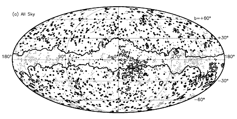
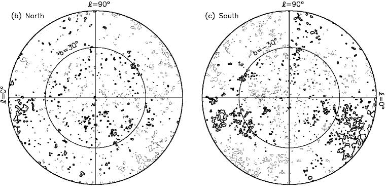
Figure 4: Iso-temperature contours of the ILC with about $1\degr$ resolution for ($a$) the whole sky, ($b$) the north, and ($c$) the south hemispheres at $\nu_{A}=-2.0$ (thick curves) and $\nu_{A}=+2.0$ (thin curves) threshold levels. Mollweide projection is used for the whole sky, where the Kp0 mask regions for removal of the strong Galactic emission and the bright radio point sources are denoted as very thick solid curves and dots. The maps for both hemispheres are stereographically projected. The temperature levels corresponding to $\nu_{A}=-2.0$ and $+2.0$ are $\Delta T=-144$ $\mu$K and $138$ $\mu$K, respectively, and have been estimated from the Kp0-masked ILC.

The northern hemisphere has very few big spots while the southern hemisphere has many.

We calculate the genus separately from the northern and the southern parts of the WMAP maps and the TCM, and also measure the genus-related statistics. The results for the observed maps and for the 500 mock observations are included in Tables 1 and 2, respectively. At the W band ($0\aas@@fstack{\circ}35$ scale), the asymmetry parameter for the southern hemisphere is very large ($\Delta g=+0.047$), which is a non-Gaussian feature that is statistically significant at $2.4\sigma$ level. However, the $\Delta g$ for the north is consistent with zero. Such a large asymmetry does not appear in the lower resolution Q and V maps.

Table 3: Genus Amplitude Differences between Northern and Southern Hemispheres for WMAP Maps

Maps	Amp. Diff.	Observed	Simulated
Kp0 mask
WMAP W	$A_{-}^{\rm N}-A_{-}^{\rm S}$	255	$17\pm 90$
	$A_{+}^{\rm N}-A_{+}^{\rm S}$	131	$15\pm 91$
WMAP V	$A_{-}^{\rm N}-A_{-}^{\rm S}$	140	$9\pm 69$
	$A_{+}^{\rm N}-A_{+}^{\rm S}$	142	$7\pm 71$
WMAP Q	$A_{-}^{\rm N}-A_{-}^{\rm S}$	108	$6\pm 51$
	$A_{+}^{\rm N}-A_{+}^{\rm S}$	103	$5\pm 53$
TCM	$A_{-}^{\rm N}-A_{-}^{\rm S}$	235
	$A_{+}^{\rm N}-A_{+}^{\rm S}$	145
ILC	$A_{-}^{\rm N}-A_{-}^{\rm S}$	56
	$A_{+}^{\rm N}-A_{+}^{\rm S}$	33
Kp0 mask & $b=30\degr$ cut
WMAP W	$A_{-}^{\rm N}-A_{-}^{\rm S}$	184	$9\pm 107$
	$A_{+}^{\rm N}-A_{+}^{\rm S}$	110	$10\pm 110$
WMAP V	$A_{-}^{\rm N}-A_{-}^{\rm S}$	107	$4\pm 83$
	$A_{+}^{\rm N}-A_{+}^{\rm S}$	125	$4\pm 86$
WMAP Q	$A_{-}^{\rm N}-A_{-}^{\rm S}$	82	$3\pm 62$
	$A_{+}^{\rm N}-A_{+}^{\rm S}$	94	$2\pm 64$
TCM	$A_{-}^{\rm N}-A_{-}^{\rm S}$	152
	$A_{+}^{\rm N}-A_{+}^{\rm S}$	93
ILC	$A_{-}^{\rm N}-A_{-}^{\rm S}$	32
	$A_{+}^{\rm N}-A_{+}^{\rm S}$	40

Figure 5$a$ shows the genus for the northern and southern hemispheres measured from the W band data. Both genus curves have different genus amplitudes, especially at the negative threshold levels. We measure amplitude differences, $A_{-}^{\rm N}-A_{-}^{\rm S}$ and $A_{+}^{\rm N}-A_{+}^{\rm S}$, from the observed W band map (Kp0-masked) and its 500 mock maps, and list the result in Table 3. Here $A_{-}^{\rm N(S)}$ is the amplitude obtained by fitting the genus points at $\nu_{A}<0$ measured in the northern (southern) hemisphere with a fitting function in equation (3), and likewise for $A_{+}^{\rm N(S)}$. The $A_{-/+}^{\rm N}-A_{-/+}^{\rm S}$ have non-zero mean values even for the Gaussian mock observations. The measured value $A_{-}^{\rm N}-A_{-}^{\rm S}=255$ for the W band map is 2.6 times larger than the standard deviation of those expected from the simulated Gaussian observations ($[255-17]/90\simeq 2.6$). On the other hand, $A_{+}^{\rm N}-A_{+}^{\rm S}$ has smaller value due to the large genus asymmetry ($\Delta g$) in the south.

We also have measured $A_{-/+}^{\rm N}-A_{-/+}^{\rm S}$ from the WMAP Q and V band maps, TCM, and ILC. From Table 3, we find that the large genus amplitude difference between the north and the south also appear at both Q and V bands (Fig. 5$b$ and 5$c$), deviating the Gaussian prediction with significance levels of about $2\sigma$ ($A_{-/+}^{\rm N}-A_{-/+}^{\rm S}=1.9\sigma$ – $2.0\sigma$), which shows that this non-Gaussian feature does not have any frequency dependence. We have computed a probability of finding such a significant deviation from the Gaussian prediction in the mock WMAP CMB fields with the Gaussian statistics. The probability that the genus curves show such a large genus amplitude differences exceeding the observed values in Table 3 at all Q, V, and W bands is only 1.4%.

Figure 5: Genus per steradian measured from the WMAP maps and the TCM for the northern (filled circles) and southern (open circles) hemispheres, together with Gaussian fitting curves (solid and dotted curves, respectively).

With a Galactic cut at $b=30\degr$, the large cold spots are removed (Fig. 4$c$). However, the trend of the genus amplitudes and asymmetries in the north and south are not significantly changed by the Galactic cuts (see Tables 1 and 3). For the Galactic cut at $b=30\degr$, $A_{-}^{\rm N}-A_{-}^{\rm S}$ and $\Delta g$ still deviate from the Gaussian prediction at $1.6\sigma$ and $1.8\sigma$ levels, respectively. Since the genus amplitude significantly decreases with higher Galactic cut, it is natural that the difference between $A_{-/+}^{\rm N}$ and $A_{-/+}^{\rm S}$ should be smaller while its standard deviation in the mock observations becomes larger due to sample variance. However, the probability that such genus amplitude differences are larger than the measured values for $b=30\degr$ cut is still 4.6%. All non-Gaussian features of the W band map described above are also seen in the TCM (Tables 1 and 3; Fig. 5$d$).

5 Origin of the Non-Gaussianity

Let us consider possible sources that may induce the non-Gaussian signatures shown in $\S 4$. First, the foreground effect on the genus may not be negligible, causing non-Gaussianity. The residual of the foregrounds after foreground-template correction is known to be very low. Bennett et al. (2003b) estimate that the residual Galactic contamination after the template correction is 2.2%, 0.8%, and $<0.4$% of the CMB power in Q, V, and W band, respectively, when the less conservative Kp2 mask is applied. Tegmark et al. (2003) also show that the foregrounds in their TCM are subdominant in all but the very innermost Galactic plane, for $\ell\la 100$. Furthermore, Galaxy foregrounds induce non-Gaussian feature by making the genus shifted to the left at all threshold levels. As for the positive $\Delta g$ on the southern hemisphere in the high resolution W band data, it is more reliable that such non-Gaussianity is caused by point sources that have not been removed by the Kp0 mask because positive $\Delta g$ means that more hot spots are present than cold spots. Furthermore, another non-Gaussian signature, the large genus amplitude difference between the north and the south, does not show frequency dependence since all WMAP band maps (Q, V, and W), ILC and TCM show the similar non-Gaussian feature. It should be noted that the three independent methods of foreground-subtraction were applied to make the WMAP band maps, ILC, and TCM. However, we cannot conclude that the non-Gaussian signatures are free from the effect of foreground contamination. The $\Delta g$ and $A_{-/+}^{N}-A_{-/+}^{S}$ decrease as the higher Galactic cut is applied, though their dependence on the Galactic cut is weak.

Second, the non-Gaussianity can appear due to the Integrated Sachs-Wolfe (ISW) and the Sunyaev-Zel’dovich (SZ) effects. The large-scale structures, which intersect the paths of CMB photons, can affect the primary CMB anisotropy. In a $\Lambda$-dominated CDM universe, the CMB anisotropies are expected to be correlated with matter density fluctuations at $z\la 2$ through the ISW effect (Crittenden & Turok 1996). Nolta et al. (2003) have detected cross-correlation of the NRAO VLA Sky Survey radio source catalog with the WMAP data. Boughn & Crittenden (2003), Fosalba & Gaztañaga (2003), Fosalba, Gaztañaga, & Castander (2003), and Scranton et al. (2003) have reported that there exists a correlation between the WMAP temperature anisotropy and the galaxy distribution. Diego, Silk, & Sliwa (2003) estimate the cross-power spectrum between the WMAP CMB and the ROSAT X-ray maps, and did not find any significant correlation between two data sets. The SZ clusters appear in arcminute scales and the angular resolution and the sensitivity of WMAP are not ideal for detection of the typical SZ effect. However, if a large number of SZ clusters contribute to the CMB map, their imprint can be statistically measurable. Recently, the positive cross-correlation between the X-ray clusters and the WMAP map has been detected. Hernández-Monteagudo & Rubiño-Martín (2003) claim their detection at $2\sigma$ – $5\sigma$ level, which corresponds to the amplitude of typically 20 – 30 $\mu$K in the WMAP map (see also Boughn & Crittenden 2003; Fosalba & Gaztañaga 2003; Fosalba et al. 2003; Myers et al. 2003).

Third, the non-Gaussian signatures may be caused by the inhomogeneous photon damping during the reionisation at the earlier epoch. Reionisation damping depends on the total optical depth $\tau$ and the angular scale subtended by the horizon at the last scattering surface defined during the reionisation epoch. The primary CMB anisotropy $\Delta T$ is damped to $\Delta Te^{-\tau}$ by the Thompson scattering with electrons, and the damping contribution to the anisotropy depends on scales. The characteristic damping scale $\ell_{r}$ is given by $\ell_{r}=(1+z_{r})^{1/2}(1+0.084\ln\Omega_{0})-1$ (Hu & White 1997; Griffiths, Barbosa, & Liddle 1999), where $z_{r}$ denotes the reionisation epoch. For $z_{r}\approx 20$ and $\Omega_{0}\approx 0.3$, the characteristic damping scale is $\ell_{r}\approx 3$. Therefore the damping is also important at low $\ell$-modes. For homogeneous reionisation, the reionisation process damps the CMB anisotropy linearly and keeps the Gaussianity of the primordial fluctuations. However, if the reionisation is inhomogeneous, for example, due to the inhomogeneous ionisation fraction or the patchy reionisation, the CMB anisotropy of low $\ell$-modes can be partially contaminated by the inhomogeneous Thompson scattering, and becomes non-Gaussian. These low $\ell$-modes (quadrupole and octopole) happen to be aligned along the Galactic plane, make the biggest spots near the Galactic plane (Tegmark et al. 2003; de Oliveira-Costa et al. 2003), and may change the temperature distributions of the Galactic north and south hemispheres differently.

Finally, the non-Gaussian signatures that have been detected may have the primordial origin. While the simple inflation predicts that the primordial fluctuation field is Gaussian, the non-linear couplings between the inflaton and the fluctuation fields or between the quantum and the classical fluctuation fields can produce weakly non-Gaussian fluctuations (Komatsu & Spergel 2001, references therein). Multi-field inflationary models predict that the primordial metric fluctuations do not need to obey Gaussian statistics (e.g., Bernardeau & Uzan 2002). There are also many mechanisms that can generate non-Gaussian density perturbations during the inflation (e.g., Bartolo, Matarrese, & Riotto 2002; Dvali, Gruzinov, & Zaldarriaga 2003).

6 Conclusions

We have investigated the topology of CMB anisotropy from the WMAP 1-year maps by measuring the genus and its related statistics. The measured WMAP genus curves clearly deviate from the Gaussian prediction in two distinctive manners. First, the genus asymmetry parameter $\Delta g$ is positive on the Galactic southern hemisphere in the WMAP W band map ($0\aas@@fstack{\circ}35$ scale), a non-Gaussian feature that is significant at $2.4\sigma$ level, while $\Delta g$ on the Galactic northern hemisphere is consistent with zero. Second, the genus amplitude difference between the north and the south hemispheres ($A_{-/+}^{\rm N}-A_{-/+}^{\rm S}$) deviates from Gaussian prediction at $2.0\sigma$ – $2.6\sigma$ levels at WMAP Q, V, and W bands. Compared to the 500 Gaussian mock observations, the observed genus amplitude differences indicate that the Gaussianity of CMB anisotropy field is ruled out at about 99% (95%) confidence level when the Kp0 mask (Kp0 mask and $b=30\degr$ Galactic cut) is applied. These non-Gaussian features have weak dependence on the Galactic cut. Similar results based on the power spectrum analysis have also been reported by Eriksen et al. (2003).

To investigate the nature of the non-Gaussian features that have been detected, we need CMB data with higher signal-to-noise ratio as well as the accurate models for the Galactic foregrounds. We wish that the next release of WMAP data or those of the future CMB experiments would enable us to resolve these problems. As for the possibility of reionisation-induced non-Gaussianity at large scales, we also need to study the topology of the CMB polarisation map (e.g., Park & Park 2002).

References

- Aghanim, Forni, & Bouchet (2001) Aghanim N., Forni O., Bouchet F.R., 2001, A&A, 365, 341
- Banday, Zaroubi, & Górski (2000) Banday A.J., Zaroubi S., Górski K.M., 2000, ApJ, 533, 575
- Bardeen et al. (1983) Bardeen J.M., Steinhardt P.J., Turner M.S., 1983, Phys. Rev. D, 28, 679
- Barreiro et al. (2000) Barreiro R.B., Hobson M.P., Lasenby A.N., Banday A.J., Górski K.M., Hinshaw G., 2000, MNRAS, 318, 475
- Bartolo, Matarrese, & Riotto (2002) Bartolo N., Matarrese S., Riotto A., 2002, Phys. Rev. D, 65, 103505
- Bennett et al. (2003a) Bennett C.L. et al., 2003a, ApJS, 148, 1
- Bennett et al. (2003b) Bennett C.L. et al., 2003b, ApJS, 148, 97
- Bernardeau & Uzan (2002) Bernardeau F., Uzan J.-P., 2002, Phys. Rev. D, 66, 103506
- Boughn & Crittenden (2003) Boughn S., Crittenden R., 2003, preprint (astro-ph/0305001)
- Bromley & Tegmark (1999) Bromley B.C., Tegmark M., 1999, ApJ, 524, 79
- Calabretta & Greisen (2002) Calabretta M.R., Greisen E.W., 2002, A&A, 395, 1077
- Chiang et al. (2003) Chiang L.-Y., Naselsky P.D., Verkhodanov O.V., Way M.J., 2003, ApJ, 590, L65
- Colley & Gott (2003) Colley W.N., Gott J.R., 2003, MNRAS, 344, 686
- Colley, Gott, & Park (1996) Colley W.N., Gott J.R., Park C., 1996, MNRAS, 281, L82
- Crittenden & Turok (1996) Crittenden R.G., Turok N., 1996, Phys. Rev. Lett., 76, 575
- de Oliveira-Costa et al. (2003) de Oliveira-Costa A., Tegmark M., Zaldarriaga M., Hamilton A., 2003, preprint (astro-ph/0307282)
- De Troia et al. (2003) De Troia G. et al., 2003, MNRAS, 343, 284
- Diego et al. (2003) Diego J.M., Silk J., Sliwa W., 2003, preprint (astro-ph/0302268)
- Dvali et al. (2003) Dvali G., Gruzinov A., Zaldarriaga M., 2003, preprint (astro-ph/0303591)
- Eriksen et al. (2003) Eriksen H.K., Hansen F.K., Banday A.J., Górski K.M., Lilje P.B., 2003, ApJ, in press (astro-ph/0307507)
- Ferreira, Magueijo, & Górski (1998) Ferreira P.G., Magueijo J., Górski K.M., 1998, ApJ, 503, L1
- Finkbeiner (2003) Finkbeiner D.P., 2003, ApJS, 146, 407
- Finkbeiner, Davis, & Schlegel (1999) Finkbeiner D.P., Davis M., Schlegel D.J., 1999, 524, 867
- Fosalba & Gaztañaga (2003) Fosalba P., Gaztañaga E., 2003, preprint (astro-ph/0305468)
- Fosalba, Gaztañaga, & Castander (2003) Fosalba P., Gaztañaga E., Castander F., 2003, ApJ, 597, L89
- Gaztañaga & Wagg (2003) Gaztañaga E., Wagg J., 2003, Phys. Rev. D, 68, 021302
- Gaztañaga et al. (2003) Gaztañaga E., Wagg J., Multamäki T., Montaña A., Hughes D.H., 2003, MNRAS, 346, 47
- Górski et al. (1999) Górski K.M., Hivon E., Wandelt B.D., 1999, in Banday A.J., Sheth R.K., da Costa L.N., eds, Proceedings of the MPA/ESO Cosmology Conference, Evolution of Large-Scale Structure: from recombination to Garching. PrintPartners Ipskamp, NL, p.37
- Gott et al. (1990) Gott J.R., Park C., Juszkiewicz R., Bies W.E., Bennett D.P., Bouchet F.R., Stebbins A., 1990, ApJ, 352, 1
- Griffiths, Barbosa, & Liddle (1999) Griffiths L.M, Barbosa D., Liddle A.R., 1999, MNRAS, 308, 854
- Guth & Pi (1982) Guth A.H., Pi S.-Y., 1982, Phys. Rev. Lett., 49, 1110
- Haslam et al. (1981) Haslam C.G.T., Klein U., Salter C.J., Stoffel H., Wilson W.E., Cleary M.N., Cooke D.J., Thomasson P., 1981, A&A, 100, 209
- Haslam et al. (1982) Haslam C.G.T., Stoffel H., Salter C.J., Wilson W.E., 1982, A&AS, 47, 1
- Hawking (1982) Hawking S.W., 1982, Phys. Lett. B, 115, 295
- Heavens (1998) Heavens A.F., 1998, MNRAS, 299, 805
- Hernández-Monteagudo & Rubiño-Martín (2003) Hernández-Monteagudo C., Rubiño-Martín J.A., 2003, MNRAS, in press (astro-ph/0305606)
- Hinshaw et al. (2003) Hinshaw G. et al., 2003, ApJS, 148, 135
- Hu & White (1997) Hu W., White M., 1997, ApJ, 479, 568
- Kogut et al. (1996) Kogut A., Banday A.J., Bennett C.L., Górski K.M., Hinshaw G., Smoot G.F., Wright E.L., 1996, ApJ, 464, 29
- Kogut et al. (2003) Kogut A. et al., 2003, ApJS, 148, 161
- Komatsu & Spergel (2001) Komatsu E., Spergel D.N., 2001, Phys. Rev. D, 63, 063002
- Komatsu et al. (2003) Komatsu E. et al., 2003, ApJS, 148, 119
- Komatsu et al. (2002) Komatsu E., Wandelt B.D., Spergel D.N., Banday A.J., Górski K.M., 2002, ApJ, 566, 19
- Magueijo (2000) Magueijo J., 2000, ApJ, 528, L57
- Melott et al. (1989) Melott A.L., Cohen A.P., Hamilton A.J.S., Gott J.R., Weinberg D.H., 1989, ApJ, 345, 618
- Mukherjee, Hobson, & Lasenby (2000) Mukherjee P., Hobson M.P., Lasenby A.N., 2000, MNRAS, 318, 1157
- Myers et al. (2003) Myers A.D., Shanks T., Outram P.J., Wolfendale A.W., 2003, preprint (astro-ph/0306180)
- Nolta et al. (2003) Nolta M.R. et al., 2003, preprint (astro-ph/0305097)
- Novikov, Feldman, & Shandarin (1999) Novikov D., Feldman H.A., Shandarin S.F., 1999, Int. J. Mod. Phys. D, 8, 291
- Page et al. (2003) Page L. et al., 2003, ApJS, 148, 233
- Pando, Valls-Gabaud, & Fang (1998) Pando J., Valls-Gabaud D., Fang L.-Z., 1998, Phys. Rev. Lett., 81, 4568
- Park et al. (1998) Park C., Colley W.N., Gott J.R., Ratra B., Spergel D.N., Sugiyama N., 1998, ApJ, 506, 473
- Park & Park (2002) Park C.-G., Park C., 2002, J. Korean Astron. Soc., 35, 67
- Park et al. (2002) Park C.-G., Park C., Ratra B., 2002, ApJ, 568, 9 (PPR)
- Park et al. (2001) Park C.-G., Park C., Ratra B., Tegmark M., 2001, ApJ, 556, 582
- Peiris et al. (2003) Peiris H.V. et al., 2003, ApJS, 148, 213
- Phillips & Kogut (2001) Phillips N.G., Kogut A., 2001, ApJ, 548, 540
- Polenta et al. (2002) Polenta G. et al., 2002, ApJ, 572, L27
- Riotto (2002) Riotto A., 2002, hep-ph/0210162
- Santos et al. (2002) Santos M.G. et al., 2002, Phys. Rev. Lett., 88, 241302
- Santos et al. (2003) Santos M.G. et al., 2003, MNRAS, 341, 623
- Seljak & Zaldarriaga (1996) Seljak U., Zaldarriaga M., 1996, ApJ, 469, 437
- Schlegel, Finkbeiner, & Davis (1998) Schlegel D.J., Finkbeiner D.P., Davis M., 1998, ApJ, 500, 525
- Scranton et al. (2003) Scranton R. et al., 2003, preprint (astro-ph/0307335)
- Shandarin et al. (2002) Shandarin S.F., Feldman H.A., Xu Y., Tegmark M., 2002, ApJS, 141, 1
- Spergel et al. (2003) Spergel D.N. et al., 2003, ApJS, 148, 175
- Starobinsky (1982) Starobinsky A.A., 1982, Phys. Lett. B, 117, 175
- Tegmark et al. (2003) Tegmark M., de Oliveira-Costa A., Hamilton A.J.S., 2003, Phys. Rev. D, 68, 123523
- Vogeley et al. (1994) Vogeley M.S., Park C., Geller M.J., Huchra J.P., Gott J.R., 1994, ApJ, 420, 525
- Wu et al. (2001) Wu J.H.P. et al., 2001, Phys. Rev. Lett., 87, 251303