Probing Dark Energy with Baryonic Acoustic Oscillations
from Future Large Galaxy Redshift Surveys

Abstract

We show that the measurement of the baryonic acoustic oscillations in large high redshift galaxy surveys offers a precision route to the measurement of dark energy. The cosmic microwave background provides the scale of the oscillations as a standard ruler that can be measured in the clustering of galaxies, thereby yielding the Hubble parameter and angular diameter distance as a function of redshift. This, in turn, enables one to probe dark energy. We use a Fisher matrix formalism to study the statistical errors for redshift surveys up to $z=3$ and report errors on cosmography while marginalizing over a large number of cosmological parameters including a time-dependent equation of state. With redshifts surveys combined with cosmic microwave background satellite data, we achieve errors of 0.037 on $\Omega_{X}$, 0.10 on $w(z=0.8)$, and 0.28 on $dw(z)/dz$ for cosmological constant model. Models with less negative $w(z)$ permit tighter constraints. We test and discuss the dependence of performance on redshift, survey conditions, and fiducial model. We find results that are competitive with the performance of future supernovae Ia surveys. We conclude that redshift surveys offer a promising independent route to the measurement of dark energy.

Submitted to The Astrophysical Journal 5-26-2003

1 Introduction

Recent observations of distant type Ia supernovae have reached the startling conclusion that the expansion of the Universe is accelerating (Perlmutter et al., 1999; Riess et al., 1998, 2001; Tonry et al., 2003). Under the premise of Friedmann equations, this implies the existence of an energy component, christened dark energy, with negative pressure (Ratra & Peebles, 1988; Frieman et al., 1995). The detailed characterization of the accelerated expansion and its cause is now one of the main subjects of cosmology. Dark energy presently constitutes about $2/3$ of the total energy density of the Universe and its physical property is often parameterized by the ratio of pressure to density, that is, the equation of state (Steinhardt, 1997; Turner & White, 1997). A cosmological constant (for a review, see Carroll, Press, & Turner, 1992) has a constant equation of state of $-1$, while general quintessence models (Caldwell et al., 1998) and other theories (Zlatev et al., 1999; Bucher & Spergel, 1999; Armendariz-Picon et al., 2000; Boyle et al., 2001; Gu & Hwang, 2001; Kasuya, 2001; Bilic et al., 2002; Deffayet et al., 2002; Freese & Lewis, 2002) typically allow equations of state with a redshift dependence. Measuring the time dependence of the equation of state, as well as its present density, is an essential step in identifying the physical origin of dark energy (Hui et al., 1999; Cooray & Huterer, 1999; Huterer & Turner, 1999; Newman & Davis, 2000; Haiman et al., 2001; Huterer & Turner, 2001; Maor, Brustein, & Steinhardt, 2001; Wang & Garnavich, 2001; Kujat et al., 2002; Maor, Brustein, McMahon, & Steinhardt, 2002; Newman et al., 2002; Weller & Albrecht, 2002; Frieman et al., 2003; Linder & Huterer, 2003). Because of the inertness and the relatively smoothness of this energy component, as commonly believed in the standard pictures of dark energy, the best cosmological probe of dark energy is the expansion history of the Universe, measured by the Hubble parameter and angular diameter distance.

In this paper, we demonstrate that the Hubble parameter $H(z)$ and angular diameter distance $D\!_{A}(z)$ can be measured to excellent precision by using the baryonic acoustic oscillations imprinted in the large-scale structure of galaxies. We are familiar with this signature as the now-famous Doppler peaks in the anisotropies of the cosmic microwave background (Peebles & Yu, 1970; Bond & Efstathiou, 1984; Miller et al., 1999; de Bernardis et al., 2000; Hanany et al., 2000; Halverson et al., 2002; Benoît et al., 2003; Bennett et al., 2003); however, the same structure is predicted to be present in the late-time clustering of galaxies as a series of weak modulations in the amplitude of fluctuations as a function of scale (Peebles & Yu, 1970; Bond & Efstathiou, 1984; Holtzman, 1989; Hu & Sugiyama, 1996). The physical scale of the oscillations is determined by the matter and baryon densities, which can be precisely measured with CMB anisotropy data. This calibrates the acoustic oscillations as a standard ruler (Eisenstein et al., 1998; Eisenstein, 2003). The observed length scales of oscillations in the transverse and line of sight directions in a galaxy redshift survey then determine the angular diameter distance $D\!_{A}(z)$ and the Hubble parameter $H(z)$ as functions of redshift. As an oscillatory feature, the acoustic signature is less susceptible to general systematic errors and distortions; however, only large surveys map enough cosmic volume to achieve the precision required to detect these features. In addition, the features along the line-of-sight clustering are on sufficiently small scales that resolving them requires an accurate measurement of redshift, motivating the need for spectroscopic redshift surveys. Surveys at higher redshift are preferred so as to avoid the erasure of the oscillatory features by nonlinear structure formation (Jain & Bertschinger, 1994; Meiksin, White, & Peacock, 1999; Meiksin & White, 1999). Recent analyses of large surveys may be beginning to reveal these features (Percival et al., 2001; Miller et al., 2001)

There have been numerous studies on how the combination of CMB anisotropy data and large-scale structure data, either present (Scott, Silk, & White, 1995; Gawiser & Silk, 1998; Lange et al., 2001; Tegmark et al., 2001; Efstathiou et al., 2002; Spergel et al., 2003) or future (Hu et al., 1998; Eisenstein et al., 1998; Wang, Spergel, & Strauss, 1999; Eisenstein et al., 1999; Popa et al., 2001), can constrain cosmological parameters. These studies have considered an increasing number of parameters and degeneracies and build on a body of work in CMB parameter estimation (Knox, 1995; Jungman et al., 1996; Zaldarriaga et al., 1997; Bond et al., 1997). However, most previous work on galaxy surveys has concentrated on low redshifts and used spherically averaged power spectra. The spherical assumption neglects the effects of redshift distortions and cosmological distortions. Including the non-isotropic information in the clustering of galaxies allows one to recover these effects (Ballinger et al., 1995; Heavens & Taylor, 1997; Hatton & Cole, 1999; Taylor & Watts, 2001; Matsubara & Szalay, 2002, 2003).

In this paper, we design large galaxy redshift surveys at high redshift that can recover the acoustic peaks with a level of precision that allows us to put competitive constraints on the dark energy. We describe the constraints in terms of statistical errors using a Fisher matrix treatment of the full three-dimensional power spectra. We study galaxy survey at $z=0.3$, $z\sim 1$, and $z=3$ so as to have access to cosmological distortions across a wide range of cosmic history. As our goal is to optimize survey design based on realistic statistical errors, we try to be conservative in our methodology. For example, we adopt ungenerous values for the non-linear scales and marginalize over a large number of cosmological parameters. We present the predicted performance of the our baseline surveys with constraints derived for $H(z)$ and $D\!_{A}(z)$ and then propagate these errors to the constraints on the dark energy parameters at our fiducial cosmology model, $\rm{\Lambda CDM}$. This work extends that of Blake & Glazebrook (2003) in that we have used a full Fisher matrix formalism to treat the cosmological constraints from large-scale structure, CMB anisotropies, and supernova data simultaneously and that we have considered time-variable equations of state. It differs from Linder (2003) in that it is an explicit treatment of the survey data sets in addition to a discussion of dark energy parameter estimation. Contemporaneously with this paper, Hu & Haiman (2003) used a Fisher matrix technique similar to ours to study the performance of a mid-redshift cluster survey. The two analyses differ in numerous details.

In § 2, we discuss the details of the physics to probe dark energy. In § 3, we present the survey condition we assume, and our Fisher information matrix methodology. We present and discuss our results in § 4. We consider variations in survey design, and fiducial model. We compare the performance to a supernovae survey (SNe) and to pure imaging surveys.

2 From Baryonic Oscillations to Dark Energy

2.1 Cosmography and Dark Energy

The expansion history of the universe can be written as the redshift $z(t)$ as a function of time, which in turn is completely specified by the Hubble parameter $H(z)$ as a function of redshift. We will probe the expansion history by measuring $H(z)$ and the angular diameter distance $D\!_{A}(z)$.

The evolution of dark energy density can be described by the present-day dark energy density $\Omega_{X}$ and the equation of state of dark energy, $w_{X}(z)$ (Steinhardt, 1997; Turner & White, 1997), where

$$w_{X}(z)=\left.\frac{p_{X}}{\rho_{X}}\right|_{z}$$ (1)

This yields an energy density as a function of redshift

$$\rho_{X}(z)=\rho_{X}(0)\exp\left[3\int_{0}^{z}\frac{1+w(z)}{1+z}dz\right]$$ (2)

Assuming a flat Universe, $D\!_{A}(z)$ and $H(z)$ are then related to the dark energy density through

$$H(z)=h\sqrt{\Omega_{m}(1+z)^{3}+\Omega_{X}\exp\left[3\int_{0}^{z}\frac{1+w(z)}{1+z}dz\right]}$$

$$=\sqrt{\frac{\Omega_{m}h^{2}}{1-\Omega_{X}}}\sqrt{\Omega_{m}(1+z)^{3}+\Omega_{X}\exp\left[3\int_{0}^{z}\frac{1+w(z)}{1+z}dz\right]}$$ (3)

$$D\!_{A}(z)=\frac{c}{1+z}\int_{0}^{z}\frac{dz}{H(z)}$$ (4)

where $\Omega_{X}$ is the present-day dark energy fraction with respect to the critical density. In a general sense, $H(z)$ and $D\!_{A}(z)$ are the fundamental observables, to be interpreted here as $\Omega_{X}$ and $w(z)$. The comoving sizes of an object or a feature at redshift $z$ in line-of-sight ($r_{\parallel}$) and transverse ($r_{\perp}$) directions are related to the observed sizes $\Delta z$ and $\Delta\theta$ by $H(z)$ and $D\!_{A}(z)$:

$$r_{\parallel} = \frac{c\Delta z}{H(z)}$$ (5)

$$r_{\perp} = (1+z)D\!_{A}(z)\Delta\theta$$ (6)

When the true scales, $r_{\parallel}$ and $r_{\perp}$, are known, measurements of the observed dimensions, $\Delta z$ and $\Delta\theta$, give estimates of $H(z)$ and $D\!_{A}(z)$. The object is then known as a “standard ruler.” Equations (5) and (6) can be applied equally well in Fourier space (inverted, of course).

It is well-known that even if we do not know the scale of a feature, we can still extract the product $H(z)D_{A}(z)$ (Alcock-Paczynski, 1979). The acoustic oscillation method presented here is not an Alcock-Paczynski method because we do know the scale of the sound horizon.

The cosmological feature to be measured need not be an actual object. Instead, we can use a statistical property of structure in many realizations such as correlation length (Ballinger et al., 1995; Matsubara & Szalay, 2003). On large scales, features in the power spectrum may be more prominent and hence easier to use.

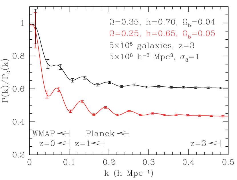
Figure 1: The linear power spectrum in two different cosmological models, $\Omega_{m}=0.35$, $h=0.70$, and $\Omega_{b}=0.04$ and $\Omega_{m}=0.25$, $h=0.65$, and $\Omega_{b}=0.05$. Each power spectrum has been divided by the zero-baryon power spectrum for that $\Omega_{m}$ and $h$. The series of acoustic oscillations is clearly seen. Lines at the bottom show the non-linear scale, shortward of which the acoustic oscillations are washed out, as a function of redshift. The scales probed by the WMAP and Planck satellite measurements of primordial anisotropy are also shown. The error bars show the spherically averaged bandpower measurements from the $z=3$ survey we will present in §3.1.

$w(z)$ can be written as a derivative of the $H(z)$ versus redshift, which in turn is a derivative of the angular diameter distance versus redshift (eq. [3] $\&$ eq. [4]). If we seek not only to measure the mean value of $w(z)$ but its slope in redshift, we are adding yet another derivative to the process. In short, to measure the time variation of the equation of state, we must be able to measure the second derivative of $H(z)$ or the third derivative of the distance-redshift relation. As each derivative magnifies the measurement noise in its parent function, we require enormous precision to proceed. In the context of galaxy surveys, this will drive us to require large volumes.

2.2 Baryonic Acoustic Oscillations in the Matter Power Spectrum

Baryonic acoustic oscillations are a generic feature of the power spectrum of large-scale structure and an excellent candidate for the standard ruler test. Prior to recombination, the baryons in the universe are locked to photons of the cosmic microwave background, and the photon pressure interacting against the gravitational instability produces a series of sound waves in the plasma. After recombination, the baryons and photons separate, but the effects of the acoustic oscillations remain imprinted in their spatial structure of the baryons and eventually the dark matter (Peebles & Yu, 1970; Holtzman, 1989; Hu & Sugiyama, 1996; Eisenstein & Hu, 1998a). The resulting power spectrum is shown in Figure 1.

The physical length scale of the acoustic oscillations depends on the sound horizon of the universe at the epoch of recombination. The sound horizon is the comoving distance a sound wave can travel before recombination and depends simply on the baryon and matter densities. The relative heights of the acoustic peaks in the CMB anisotropy power spectra measure these densities to excellent accuracy, thereby producing an accurate measurement of the sound horizon (Eisenstein et al., 1998; Eisenstein, 2003).

While the matter power spectrum is simply a product of the spectrum of primordial fluctuations and the modification of those fluctuations in later epochs, notably the radiation-domination era and recombination, our observations of this power spectrum are complicated by the biases of galaxy clustering, the distortions from peculiar velocities, and the errors induced from reconstructing distances with the wrong cosmology. The latter two effects break the intrinsic statistical isotropy of the clustering of matter and introduce variations that depend on the angle of the wavevector to the line of sight.

In the absence of massive neutrinos (Bond & Szalay, 1983), linear perturbation theory fixes the shape of the matter power spectrum in comoving coordinates and changes only the amplitude as the structure evolves. The growth function $G(z)$ rescales the amplitude of the fixed matter power spectrum to account for the growth of structure from the recombination to a redshift $z$. The growth function does depend on the details of dark energy. However, the subtle changes in the amplitude of the matter power spectrum are easily confused in galaxy redshift surveys with evolution in the bias of galaxies. While bias can be estimated from redshift distortions, recovering it to the $1\%$ accuracy required for interesting constraints on dark energy is unlikely, especially in light of the systematic uncertainties of poorly known scale-dependencies of the redshift distortion.

In principle, galaxy clustering bias could be arbitrary (Dekel & Lahav, 1999); however, under the assumptions of local bias and Gaussian statistics for the density field, the bias on large scales should be independent of scale in the correlation function (Coles, 1993; Scherrer & Weinberg, 1998; Meiksin, White, & Peacock, 1999; Coles et al., 1999). In the power spectrum, this appears as a constant multiplicative bias plus a constant additive offset (Seljak, 2000). Moreover, even if the bias deviates from scale independence on linear or quasi-linear scales, it is very implausible for it to introduce oscillations in Fourier space on the acoustic scales, as this would correspond to a preferred length scale in real space of enormous size ($\gtrsim 30{\rm\;Mpc}$).

Redshift distortions are an angle-dependent distortion in power caused by the peculiar velocities of galaxies (Hamilton, 1998, and references therein). On the largest scales, these distortions follow a simple form (Kaiser, 1987) in which the distortion is an angle-dependent, multiplicative change in power. We will follow this prescription. In reality, redshift distortions are non-linear, including the finger of God effects on small scales. However, these deviations have no large preferred length scale and will not disturb analysis of the acoustic oscillations.

Whereas the linear-theory redshift distortions are an angle-dependent modulation in the power spectrum amplitude, the cosmological distortion resulting from an incorrect mapping of observed separations to true separations produces a distortion in scale. Spherical features in power become ellipsoids under the false cosmology. Were the power spectrum a simple power law, the cosmological and redshift distortions would be indistinguishable in their quadrupole signatures and difficult to separate overall. Fortunately, the matter power spectrum is not a simple power law and the slow rollover in the power lifts some of the degeneracy between the two distortions (Ballinger et al., 1995; Matsubara & Szalay, 2003). However, strong features such as baryonic acoustic oscillations are far more powerful at separating the two, because with a rapidly varying function, the difference between dilating the scale and modulating the amplitude is very stark.

Unfortunately, the use of baryonic oscillations as a standard ruler to derive $D\!_{A}(z)$ and $H(z)$ is not always straightforward. The nonlinear gravitational growth of perturbation in the large scale structure erases the primordial features on smaller scales (large wavenumbers). This occurs when perturbations on a given scale become of order unity in amplitude, leading to non-linear coupling between Fourier modes. The obscuration by nonlinearity moves to a larger scale as the Universe evolves, and today, the scale corresponds to wavelengths of about 60$h^{-1}{\rm\;Mpc}$, enough to wipe out all but the first and a part of the second of the acoustic oscillations (Meiksin, White, & Peacock, 1999). At higher redshift, the process is less advanced, and we can recover the primordial signals on smaller scales, including the full series of acoustic oscillations. For example, at $z=3$, we should be able to recover primordial information to roughly 12$h^{-1}{\rm\;Mpc}$ (a factor of two smaller than what can be found in the primary anisotropies of the microwave background), which means that many acoustic oscillations can be preserved outside of nonlinearity region. In practice, we will be limited to about four peaks because Silk damping makes the higher harmonics smaller than our expected power spectrum measurements. Figure 1 shows the non-linear scale as a function of redshift, as well as the scales probed by the CMB primary anisotropies as measured by the WMAP and Planck satellites. While low-redshift surveys such as the Sloan Digital Sky Survey (York et al., 2000) are much more restricted by the nonlinearity of clustering, they do provide a valuable data point at an epoch where the dark energy is largest.

It is worth comparing the measurements from future redshift surveys to those inferred from the observations of type Ia supernovae (hereafter SNe) (Riess et al., 1998; Perlmutter et al., 1999; Riess et al., 2001; Tonry et al., 2003). The SNe survey measure the luminosity distance as a function of redshift, which in standard cosmologies is equivalent to the angular diameter distance. While this requires an additional derivative to extract $w(z)$ relative to measures of $H(z)$, future SNe program such as the SNAP satellite could achieve extremely good precision on distances at redshifts below 1.7. While the cosmological implications of low-redshift acoustic oscillations and SNe distances are partially degenerate, the systematic errors will be completely different.

In summary, the baryon acoustic oscillations form a standard ruler that can be measured through galaxy redshift surveys to yield $H(z)$ and $D_{A}(z)$ at a range of redshifts. The scale of the acoustic oscillations is expected to be very robust to non-linear gravitational clustering, galaxy biasing, and redshift distortions, making this a potentially clean probe of cosmography. If we can show that the distance measurements can be made to sufficient precision, then acoustic oscillations will offer an new and independent path to the quantification of dark energy.

3 Methodology

In this section, we present the methodology of constraining the dark energy through distance measurements derived from surveys of galaxy clustering. To probe the time evolution of the dark energy, we need galaxy power spectra at a variety of redshifts. We design surveys at six different redshift bins, ranging from 0.3 to 3. In this section, we present our methodology for computing the statistical errors from these surveys and from our ancillary data sets. We do this using a Fisher matrix formalism in a parameterized cosmological model.

3.1 Statistical Error on the Power Spectrum

To estimate errors on $D\!_{A}(z)$ and $H(z)$, we begin with the errors on the power spectrum that result from a galaxy survey. Under Gaussian approximations, the statistical errors are a combination of the limitations of the finite volume of the survey and the incomplete sampling of the underlying density field. These are known as sample variance and shot noise, respectively. At a single wavevector $\vec{k}$, the intrinsic statistical error associated with power is the sum of the power and shot noise (Feldman, Kaiser, & Peacock, 1994; Tegmark, 1997)

$$\frac{\sigma_{P}}{{P}}=\frac{P+\frac{1}{n}}{P}$$ (7)

Here, $1/n$ is a white shot noise from the Poisson sampling of the density field assuming that the comoving number density $n$ is constant in position. If the shot noise term exceeds the true power, that is, when $nP$ is less than unity, then shot noise will significantly compromise the measurement. Note that $nP$ depends on wavenumber.

However, when the survey volume is finite, the power at nearby wavevectors is highly correlated, and one can think of discretizing the Fourier modes of the density field into cells in Fourier space whose volume is $(2\pi)^{3}/V_{\rm survey}$, where $V_{\rm survey}$ is the comoving survey volume. Neglecting boundary effects, the statistical power of the survey is well approximated by treating these cells as independent (Tegmark, 1997). If the survey volume is large enough that the discretization scale is small compared to the regions of wavevector space over which the power spectrum is constant, then we can estimate the bandpower as averaged over a finite volume in Fourier space. We parameterize this by the wavenumber range $\Delta k$ and the range $\Delta\mu$ of the cosine of the angle between the wavevector and the line of sight. The volume in Fourier space is simply $2\pi k^{2}\Delta k\Delta\mu$ and the number of modes is $2\pi k^{2}\Delta k\Delta\mu V_{\rm survey}/(2\pi)^{3}$. However, because the density field is real-valued, the Fourier modes $\vec{k}$ and $-\vec{k}$ are not independent, which reduces the number of independent modes by a factor of two. The fractional error on the bandpower is then (Feldman, Kaiser, & Peacock, 1994; Tegmark, 1997):

$$\frac{\sigma_{P}}{P}=2\pi\sqrt{\frac{2}{V_{\rm survey}k^{2}\Delta k\Delta\mu}}\left(\frac{1+nP}{nP}\right)$$ (8)

where $P$ is the average comoving bandpower. This fractional error on power spectrum (eq. [8]) enters in Fisher matrix and will be propagated to the errors on parameters which we want to calculate.

3.2 The Fisher Information Matrix for Galaxy Redshift Surveys

Given the uncertainties of our observations, we now want to propagate these errors to compute the precision of constraints on cosmological parameters. The Fisher information matrix provides a useful method for doing this (see Tegmark, Taylor, & Heavens, 1997, for a review). The method takes as input a set of observables and a parameterized theoretical model to predict those observables. We denote the parameters as $p_{1},\ldots,p_{N}$. The Fisher information matrix incorporates the likelihood function of the observables to yield the minimum possible errors on an unbiased estimator of a given parameter, given that the true value of the parameters are that of a so-called fiducial model. Mathematically, these minimum errors are simply the square roots of the diagonal elements of the inverse of the Fisher matrix.

Assuming the likelihood function for the bandpowers of a galaxy redshift survey to be Gaussian, the Fisher matrix can be approximated as (Tegmark, 1997)

$$F_{ij} = \int_{\vec{k}_{\rm min}}^{\vec{k}_{\rm max}}\frac{\partial\ln P(\vec{k})}{\partial p_{i}}\frac{\partial\ln P(\vec{k})}{\partial p_{j}}V_{\rm eff}(\vec{k})\frac{d\vec{k}}{2(2\pi)^{3}}$$

$$= \int_{-1}^{1}\int_{k_{\rm min}}^{k_{\rm max}}\frac{\partial\ln P(k,\mu)}{\partial p_{i}}\frac{\partial\ln P(k,\mu)}{\partial p_{j}}V_{\rm eff}(k,\mu)\frac{2\pi k^{2}dkd\mu}{2(2\pi)^{3}}$$

where the derivatives are evaluated at the parameter values of the fiducial model and $V_{\rm eff}$ is the effective volume of the survey, given as

$$V_{\rm eff}(k,\mu) = \int\left[\frac{{n}(\vec{r})P(k,\mu)}{{n}(\vec{r})P(k,\mu)+1}\right]^{2}d\vec{r}$$ (10)

$$= \left[\frac{{n}P(k,\mu)}{{n}P(k,\mu)+1}\right]^{2}V_{\rm survey},$$

where the last equality holds only if the comoving number density $n$ is constant in position. Here, $\mu=\vec{k}\cdot\hat{r}/k$, where $\hat{r}$ is the unit vector along the line of sight and $\vec{k}$ is the wave vector with norm $k=|\vec{k}|$. Due to azimuthal symmetry around the line of sight, the power spectrum $P(\vec{k})$ depends only on $k$ and $\mu$, but of course it has an implicit dependence on the cosmological parameters $p_{i}$. Equations (3.2) and (10) are not fully general, as we have assumed a flat-sky approximation in which the survey box is imagined to be far from the observer. Given that the clustering scales of interest will subtend small angles on the sky in all of our designed surveys, this is an appropriate approximation.

We have not included information from all wavenumbers in our equation (3.2). Wavenumbers smaller than $k_{\rm min}$ or larger than $k_{\rm max}$ have been dropped. We use $k_{\rm max}$ to exclude information from the non-linear regime, where our linear power spectra are inaccurate. We adopt conservative values for $k_{\rm max}$ by requiring $\sigma(R)=0.5$ at a corresponding $R=\pi/2k$. At $z=0$, this sets $k_{\rm max}=0.1h{\rm\;Mpc^{-1}}$, which is consistent with the numerical simulations of Meiksin, White, & Peacock (1999) and noticeably smaller than that used by most published analysis of past redshift surveys. The $k_{\rm max}$ values used for different redshift bins are listed in Table 1. The maximum scale of the survey $k_{\rm min}$ has almost no effect on the results; we adopt $k_{\rm min}=0$.

In principle, the mapping from the observed galaxy separations to the physical separations and wavevectors depends upon the cosmological functions $D_{A}(z)$ and $H(z)$, which are varying continuously across the redshift range of the survey. When doing an analysis of real data, one would of course include this variation. For our forecasts, however, we opt to break the survey into a series of slabs in redshift, inside of which we treat the survey region as a fixed Euclidean geometry, with a constant $D_{A}$ and $H$ and a rectilinear division between the transverse and radial directions. This approximation is harmless as regards the statistical power of the survey or the parameter degeneracies involved. We use redshift bins that are narrow enough to finely sample the dark energy behavior.

3.3 Parameters

A Fisher matrix formalism relies upon a detailed parameterization of its space of models. The performance forecasts are only as realistic as the generality of the permitted models. For our forecasts, we proceed in two stages. First, we define a very general parameterization based on CDM cosmologies and assigning independent parameters to each redshift bin. This permits us to forecast cosmographical constraints independent of any dark energy model. Second, we introduce a smaller set of parameters to describe dark energy by relating the distances in different redshift bins. This will allow us to combine many distance measurements into constraints on a low-dimensional dark energy model.

3.3.1 Cold Dark Matter Cosmography

We use a very general space of cold dark matter models. Our parameter include the matter density ($\Omega_{m}h^{2}$), baryon density ($\Omega_{b}h^{2}$), matter fraction($\Omega_{m}$), the optical depth to reionization ($\tau$), the spectral tilt ($n_{s}$), the tensor-to-scalar ratio ($T/S$), and the normalization ($\ln{A_{S}}^{2}$). Our fiducial model is $\Omega_{m}=0.35$, $h=0.65$, $\Omega_{\Lambda}=0.65$, $\Omega_{K}=0$, $\Omega_{b}h^{2}=0.021$, $\tau=0.05$, tilt, $n_{s}=1$, and $T/S=0$.

We supplement this model with many additional parameters to describe the behavior at each redshift. For the CMB, we include an unknown angular distance $D_{A,\rm CMB}$ to the last scattering surface at $z=1000$. For each redshift survey bin, we add a parameter for the angular diameter distance ($\ln D_{A}$), the Hubble parameter ($\ln H$), the linear growth function ($\ln G$), the linear redshift distortion ($\ln\beta$), and an unknown shot noise $P_{\rm shot}$. With 5 additional parameters in each of 6 redshift bins, the total number of parameters for the CMB and galaxy surveys is 38. The fiducial values of these parameters are evaluated at the central redshift of each slice, and the fiducial values of $\beta$ are computed from the values of the bias as found from the fiducial values of the observed galaxy clustering.

By keeping $D\!_{A}(z)$, $H(z)$, and $G(z)$ as separate parameters at each redshift, we have avoided any assumption thus far of a specific dark energy model. The only cross-talk between the various distances and amplitudes occurs through the parameters of $\Omega_{m}h^{2}$, $\Omega_{b}h^{2}$, and $n_{s}$ that set the shape of the galaxy power spectrum. In other words, a good constraint at one redshift implies nothing for another redshift because we have specified nothing about the behavior of the distances as a function of redshift.

The unknown white shot noise $P_{\rm shot}$ is a shot noise in the observed power spectrum at each redshift bin that remains even after the conventional shot noise of inverse number density is subtracted from the observed power spectrum. These terms can arise from galaxy clustering bias (Seljak, 2000) even on large scales because they zero-lag terms in the correlation function, which are permitted in the theories of local bias (Coles, 1993).

The partial degeneracy between redshift distortions and cosmological distortions requires care because the broadband aspects of the observed power spectra are extremely well-constrained in these surveys. If one knew the precise amplitude of the matter power spectrum at a given redshift, then one would know the bias to high precision. This would yield the value of $\beta$, and knowing this, we could extract the cosmological distortions from the quadrupole distortions of the observed power. Unfortunately, we do not regard this as a robust cosmological test. Non-linear redshift distortions are not well understood, particularly in the context of poorly constrained bias models. We seek to isolate our measurement of the cosmological distortions from overly optimistic assumptions about redshift distortions. The unknown growth functions and shot noises aid in this separation; the latter contributes because a white noise limits the localization of a power-law break in a smooth power spectrum. We do not use the recovered growth functions in our dark energy fits. We will return to this topic in § 4.4

3.3.2 From Cosmography to Dark Energy

We next wish to define a more restricted parameterization for the study of dark energy. We do this through a simple parameterization for the equation of state $w(z)$. The equation of state of a cosmological constant has $w=-1$ at all times, whereas quintessence models have $w>-1$, generically with time dependence. While the most important distinction of dark energy models would be to decide whether $w=-1$ or not, we also want to develop methods for tracking the time dependence. As a simplest approach, we assumed a linear equation of state in redshift (eq. [11]).

$$w(z)=w_{0}+w_{1}z$$ (11)

Our choice of parameters for a dark energy is $\Omega_{X}$ (eq. [3]), $w_{0}$, and $w_{1}$. Other choices for parameterizing the free function $w(z)$ have been explored in Tegmark (2001), Linder (2003), and Huterer & Starkman (2003).

We used a variety of dark energy fiducial models in this paper. The parameters of these models are listed in Table 2. We will focus most of our attention on a $\rm{\Lambda CDM}$ model with $\Omega_{X}=0.65$, $w_{0}=-1$, and $w_{1}=0$ and on a comparison model (Model 2) with $w_{0}=-2/3$. The primary difference between these is that dark energy remains more important at higher redshift in the $w=-2/3$ model. We consider four models with redshift-dependent equations of state. All have $w_{1}>0$, so that dark energy emerges at higher redshift than we would infer from $w$ today. In detail, we truncate the increase in $w$ at early times by setting $dw/dz=0$ at $z>2$ so that the value of $w$ at $z>2$ is simply $w(2)$. This is of minor importance because the dark energy is subdominant at these high redshifts, but it is necessary to avoid dark energy domination at early times. Models 5 and 6 have $w<-1$ today, which is a challenge to theory (but see Caldwell et al., 1998); we include these simply to study the phenomenological differences.

Equation (11) defines the equation of state today as the parameter $w_{0}$. Because the observations are all at higher redshift, the errors on $w_{0}$ are misleadingly poor, because uncertainties in $w_{1}$ allow the value today to vary around a well-measured value at higher redshift. Errors on $w$ at higher redshifts decrease to a minimum at a redshift $z_{\rm pivot}$, similar to the central redshift of the observations, and then increase again. For any choice of $z_{\rm pivot}$, we can recast the parameterization in equation (11) as

$$w(z)=w_{0}+w_{1}z=w(z_{\rm pivot})+w_{1}(z-z_{\rm pivot})$$ (12)

At this redshift of minimum error, the covariance between $w(z_{\rm pivot})$ and $w_{1}$ vanishes, so that the two parameters are statistically independent. $z_{\rm pivot}$ can be computed from the covariance matrix of $w_{0}$ and $w_{1}$ via the method in Appendix A of Eisenstein et al. (1999).

3.4 Completion and Transformation of Fisher Matrices

We must complete our formula (eq. [3.2]) for the Fisher information matrix for galaxy surveys by identifying the power spectrum for the corresponding redshift bin. $P(\vec{k})$ in equation (3.2) is a three-dimensional galaxy redshift power spectrum, to be reduced to two dimensions by symmetry. When we reconstruct our measurements of galaxy redshifts and positions using a particular reference cosmology, which differs from the true cosmology, the observed power spectrum is

$$P_{\rm obs}(k_{{\rm ref}\perp},k_{{\rm ref}\parallel})=\frac{D\!_{A}(z)_{\rm ref}^{2}\times H(z)}{D\!_{A}(z)^{2}\times H(z)_{\rm ref}}P_{\rm true}(k_{\perp},k_{\parallel})+P_{\rm shot}.$$ (13)

Here, $D_{A}$ and $H$ values in the reference cosmology are distinguished by the subscript ‘ref’, while those in the true cosmology have no subscript. $k_{\perp}$ and $k_{\parallel}$ are the wavenumbers across and along the line of sight in the true cosmology. These are related to the wavenumbers calculated assuming the reference cosmology, by $k_{{\rm ref}\perp}=k_{\perp}D_{A}(z)/D_{A}(z)_{\rm ref}$ and $k_{{\rm ref}\parallel}=k_{\parallel}H(z)_{\rm ref}/H(z)$. The prefactor of distance ratios accounts for the difference in volume between the two cosmologies. We adopt the reference cosmology to be equal to our fiducial cosmology for simplicity.

Next, the true cosmology must be constructed, included the redshift distortions. We do this by scaling to $z=0$:

$$P_{\rm obs}(k_{{\rm ref}\perp},k_{{\rm ref}\parallel})=\frac{D\!_{A}(z)_{\rm ref}^{2}H(z)}{D\!_{A}(z)^{2}H(z)_{\rm ref}}b^{2}\;\left(1+\beta\frac{k^{2}_{\parallel}}{k^{2}_{\perp}+k^{2}_{\parallel}}\right)^{2}$$

$$\quad\quad\quad\times\left(\frac{G(z)}{G(z=0)}\right)^{2}P_{{\rm matter},z=0}(k)+P_{\rm shot}$$ (14)

where the bias $b$ is $\Omega_{m}(z)^{0.6}/\beta(z)$. The normalization used to derive the power spectrum at z is,

$$P(k_{\rm norm},z=1000)=A_{S}^{2}\frac{k_{\rm norm}}{k_{\rm fid}}\left(\frac{c}{H(1000)}\right)^{4}$$ (15)

where $k_{\rm fid}=0.025/{\rm\;Mpc}$ and $k_{\rm norm}^{-1}=3000{\rm\;Mpc}$. The actual power spectrum and derivatives with respect to various parameters are reconstructed from equation (14), using the numerical methods and results at $z=0$ from Eisenstein et al. (1999).

For the Fisher matrix of CMB, we assume errors for the Planck satellite including polarization from Eisenstein et al. (1999). With Planck, the fractional error on $\Omega_{m}h^{2}$ and $\Omega_{b}h^{2}$ are 0.9% and 0.6%, respectively. Together, these more than suffice to calibrate the sound horizon to 1%. The recovered error on the angular diameter distance to $z=1000$ is 0.2%.

Figure 2: A flowchart of transformations of the Fisher matrices necessary to produce forecasts for the distance and dark energy parameters.

For the Fisher matrix of SNe, we introduce 16 redshift bins, at 0.05 and at 0.3 to 1.7 by steps of 0.1, to represent the supernovae distance information. We assign 1% independent errors to each redshift point (i.e., 0.022 mag error in distance modulus), with an overall 5% uncertainty in the distance scale (since the SNe method by itself gives only a relative distance measurement). The appropriate covariance matrix is constructed and then inverted to give the Fisher matrix. In practice, the uncertainty in the distance scale is substantially reduced from the 5% starting value by combination with the CMB, because the CMB’s measurement of $\Omega_{m}h^{2}$ is combined with the SNe measurement of $\Omega_{m}$ to yield the Hubble constant itself.

Figure 3: Derivatives of angular diameter distance($D_{A}$) and Hubble parameter($H$) with respect to $\Omega_{X}$, $w_{0}$, and $w_{1}$ with $\Omega_{m}h^{2}$ being held fixed. As these are partial derivatives, one should remember that two of the three parameters are held fixed as well in each case. Notably, these are not the basis that leave the CMB anisotropies unchanged. The $\Omega_{X}$ parameter is equivalent to $\Omega_{m}$. Left: $w=-1.0$ ($\rm{\Lambda CDM}$). Right: $w=-0.667$ (Model 2).

Our SNe model was chosen to give similar performance to that of the proposed SNAP mission (Aldering et al., 2002) but differs in fine detail from that of the SNAP team. One should note that our 16 redshift points are statistically independent, so that with modest rebinning we are asserting better than 0.01 mag calibration between low and high redshift SNe. This is well beyond the current state of the art and is essentially the design goal of the SNAP mission.

Once the Fisher matrices for all the constituent data sets are set, we must derive marginalized errors on $D\!_{A}(z)$ and $H(z)$ and eventually on the dark energy parameters. Figure 2 shows the steps of the procedure graphically. To begin, the Fisher matrices are summed up and inverted. The square roots of the diagonal terms of this inverse Fisher matrix are the marginalized errors on parameters. We marginalize over and remove all the parameters that are not concerned with cosmography by taking a submatrix of the inverse Fisher matrix that includes only the rows and columns for $\Omega_{m}h^{2}$, $D_{A,\rm CMB}$, and the $H(z)$’s and $D\!_{A}(z)$’s at all redshift bins. This yields the covariance matrix for the cosmographical parameters. Although this is an intermediate result, it is very useful because it is independent of any dark matter model.

Next we project these errors through to the dark energy parameter space. Because the dark energy model makes explicit predictions for the various distances, we are not marginalizing over parameters. Rather, we are contracting the inverse of the covariance matrix, as one would do in a multi-dimensional $\chi$-square analysis. Hence, we invert the cosmographic covariance matrix to get a Fisher matrix $\overline{F}$ and contract this with the set of derivatives between the the distances and the dark energy parameters ($\Omega_{m}h^{2}$, $\Omega_{X}$, $w_{0}$, and $w_{1}$).

$$\overline{F}_{{\rm DE},ij} = \sum_{m,n}\frac{\partial p_{n}}{\partial q_{i}}\overline{F}_{nm}\frac{\partial p_{m}}{\partial q_{j}},$$ (16)

where the $p_{m}$ are the distance parameters and the $q_{i}$ are the dark energy parameters. By inverting this Fisher matrix, we attain marginalized errors of dark energy parameters.

Equation (16) implies that the constraints on dark energy will be a combination of how well $D\!_{A}(z)$ and $H(z)$ are estimated within a given set of surveys and how effectively measurements of $D\!_{A}(z)$ and $H(z)$ can constrain dark energy. Figure 3 shows the derivatives of $D_{A}(z)$ and $H(z)$ with respect to the dark energy parameters. The left panel is for $\rm{\Lambda CDM}$; the right panel is for Model 2 ($w=-2/3$). One should remember that these are partial derivatives, so that three of the parameters $\Omega_{m}h^{2}$, $\Omega_{X}$, $w_{0}$, and $w_{1}$ are being held fixed. The derivatives with respect to $w_{0}$ at fixed $\Omega_{m}h^{2}$, $\Omega_{X}$ and $w_{1}$ have larger amplitude than those to $w_{1}$, meaning that $D_{A}$ and $H$ place better constraints on $w_{0}$ than on $w_{1}$. Based on the positions of maximum amplitudes, we expect that the information on $w_{1}$ comes from higher redshift than $w_{0}$. It is interesting to note that while an advantage of this acoustic oscillation method is to measure $H(z)$, the peaks of derivatives of $H(z)$ are at lower redshift where, as we will find, this method has poorer error bars. This tends to favor lower redshift probes such as SNe. It also implies that, improving error bars on $w_{1}$ could be done by changing the redshift survey conditions at higher redshifts, that is, we may want to decrease error bars on $H(z)$ over the range $z=1$ to 3 or on $D\!_{A}(z)$ at $z\gtrsim 2$. Comparing $w=-2/3$ to $\rm{\Lambda CDM}$, one finds that the derivatives of both $D\!_{A}(z)$ and $H(z)$ peak at higher redshift when $w$ is more positive. This will favor the galaxy surveys at higher redshift. Models 3 through 6 share this trend.

3.5 Survey Design

We want to design redshift surveys that are optimized to derive $D\!_{A}(z)$ and $H(z)$ within accessible resources. Our requirement is that we should be able to measure multiple acoustic peaks at various redshifts with high precision. In this section, we define two sets of baseline surveys, with parameters in Table 1; we will also consider variations on these in § 4.

To constrain the scale of the acoustic peaks, we clearly need superb precision in the power spectrum measurements. Equation (8) shows that the errors $\sigma_{P}$ depend on the survey volume $V_{\rm survey}$ and on the number density $n$ of objects in the survey. Of course, $V_{\rm survey}$ and $n$ are limited by the available observational resources. If we assume that the observational resources scale with the total number of objects $N$, then at fixed $N$, $\sigma_{P}/P$ has a minimum at $n=1/P$ (Kaiser, 1986) at each wavenumber $k$. However, near this minimum, the performance $\sigma_{P}/P$ varies slowly, and a small deviation from the minimum incurs little penalty. For example, using $nP=3$ or $nP=1/3$ increase the error by only about 15%. With the relatively small dependence of error on $nP$ near the minimum, we suggest that $nP$ slightly larger than 1 is preferable for several reasons. First, larger $nP$ increase the signal-to-noise per pixel in the map. This enables computations beyond the power spectrum, e.g. for higher-order correlations and non-Gaussianity. Second, it avoids some complication from the non-Gaussianity of the shot noise itself. Finally, it permits us to the survey into a few sub-samples based on galaxy properties or other criteria with less loss in signal-to-noise. This allows certain kinds of tests for systematic errors in the survey and for additional science return from the study of type-dependent galaxy bias.

On the other hand, it is possible that observation resources do not simply scale with the number of objects. For example, the field of view, i.e. $V_{\rm survey}$, may be more expensive than the number of spectroscopic targets. For a fixed survey volume, the error bars improve monotonically as targets are added, but the benefit saturates at $nP\gg 1$. For example, the error $\sigma_{P}/P$ with $nP=5$ is 1.7 times better than that of $nP=1$ (at fixed volume), but only 20% worse than that of $nP=\infty$. In reality, increased target density is not free: hence higher number densities of objects require fainter objects (i.e., a deeper survey) and hence longer exposure times. Fortunately, the range of the number density we want is near the luminous tale of the luminosity functions, where the source counts are quite steep, and so it is rather easy to increase $n$ moderately above $1/P$.

We conclude that $nP\sim 3$ is a good choice based on these considerations.

An additional question is which wavenumber $k$ to use in calculating the value of $nP$. We are primarily interested in higher acoustic peaks, which occur around $k=0.2h{\rm\;Mpc^{-1}}$. The power at this wavenumber is about 2500$\sigma^{2}_{8,g}h^{-3}{\rm\;Mpc}^{3}$, where $\sigma^{2}_{8,g}$ is the rms overdensity of the galaxies in spheres of 8$h^{-1}{\rm\;Mpc}$ comoving radius. This gives $n=4\times 10^{-4}\sigma^{-2}_{8,g}h^{3}{\rm\;Mpc}^{-3}$ for $nP=1$. This is considerably less than the density of $L^{*}$ galaxies. Power is higher at smaller $k$, so smaller densities would be optimal when measuring larger scales.

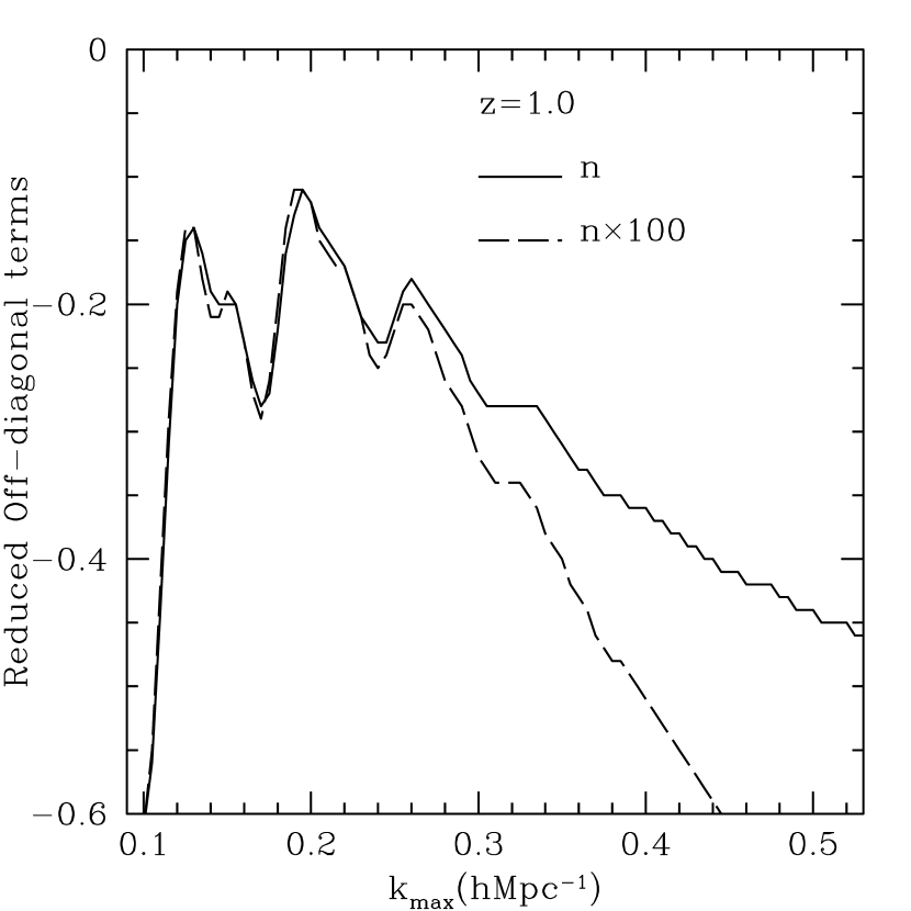
Figure 4: Errors on $D\!_{A}(z)$ and $H(z)$ as a function of $k_{\rm max}$ and $n$ for $z=1$ data set. $n$ means the baseline number density in Table 1 (about $5\times 10^{-4}h^{3}{\rm\;Mpc}^{-3}$), and $n\times 100$ means 100 times the baseline number density.

At $z\sim 3$, the obvious choice of galaxy targets are the Lyman-break galaxies (Steidel et al., 1996). $\sigma_{8,g}$ for these galaxies is measured to be about 1 (Steidel et al., 1998; Adelberger et al., 1998). The corresponding bias is calculated using

$$\sigma_{8,g}=b\sigma_{8,\rm mass}\sqrt{1+\frac{2\beta}{3}+\frac{\beta^{2}}{5}}$$ (17)

assuming $\sigma_{8,\rm mass}$ of 0.9 for the matter distribution today and a linear redshift distortion effect (Kaiser, 1987). For the number density, $10^{-3}h^{3}{\rm\;Mpc}^{-3}$ is used so that $nP\approx 3$ at $k=0.2h{\rm\;Mpc^{-1}}$. As an aside, a density $nP(0.2h{\rm\;Mpc^{-1}})>1$ is particularly valuable at $z=3$ because the non-linear scale has receded to much smaller scales ($k_{\rm max}\approx 0.5h{\rm\;Mpc^{-1}}$!). To make full use of the survey at all linear scales, we need a larger $n$. For our baseline survey, we adopt a total comoving volume of 0.5$h^{-3}{\rm Gpc^{3}}$, which gives enough resolution and the precision to recover the first four acoustic peaks (Figure 1). At this redshift, the comoving volume between $z=2.5$ and $z=3.5$ is 960$h^{-3}{\rm\;Mpc}^{3}$ per square arcminute, yielding a total survey field of 140 square degrees. The areal number density is 1 galaxy per square arcminute, similar to the depth of Steidel et al. (1998).

At $z\sim 1$, the choice of galaxy target is less obvious. One could reasonably use either giant ellipticals or luminous star-forming galaxies. Luminous early-type galaxies have the advantage of high bias, probably $\sigma_{8,g}>1$, and strong 4000Å breaks, but getting the redshift does require detecting this continuum break, which takes longer integration time. Later-type galaxies may be less biased, meaning we need a larger number density, but they have strong 3727Å emission lines, which can often be identified because the line is a doublet. For either case, we assume $\sigma_{8,g}=1$ and $n=5\times 10^{-4}h^{3}{\rm\;Mpc}^{-3}$. This makes $nP$ at $k\sim 0.2h{\rm\;Mpc^{-1}}$ slightly bigger than 1, which means that $nP$ will be at our desired value for the meaty part of the linear regime. From $z=0.5$ to $z=1.3$, there is a comoving volume of $480h^{-3}{\rm\;Mpc}^{3}$ per square arcminute, leading to a surface density of 0.24 galaxies per square arcminute. We assumed total survey field of 1000 square degree, chosen to sample a similar volume to the Sloan Digital Sky Survey (SDSS) luminous red galaxy sample. The total number of galaxies is 8.7$\times 10^{5}$. To ensure sufficient resolution on the variations of $D\!_{A}(z)$ and $H(z)$, we subdivide the $z\sim 1$ survey into four redshift bins centering at $z=$0.6, 0.8, 1.0, 1.2 with widths $\Delta z=0.2$. Hereafter, unless noted, the term ‘$z\sim 1$ survey’ designates the sum of these four redshift bins.

For the nearby universe, we adopt the parameters of the on-going SDSS luminous red galaxy survey (Eisenstein et al., 2001). The survey volume for this sample is 1$h^{-3}{\rm Gpc^{3}}$, and the comoving number density is $10^{-4}h^{3}{\rm\;Mpc}^{-3}$ at $z\approx 0.3$. This survey is included in all analyses in this paper because it is well underway. We use $\sigma_{8,g}=1.8$ for these galaxies.

To resolve the oscillations along the line of sight at $k\approx 0.2h{\rm\;Mpc^{-1}}$, and thereby measure $H(z)$, requires that the position of the galaxy along the line of sight be well estimated. As the crest-to-trough distance for this wavelength is only $15h^{-1}{\rm\;Mpc}$, we need redshifts with accuracy of $10^{-3}$ in $1+z$. We will return to this computation in § 4.5, but for now we note that this accuracy requires low-resolution spectroscopy. Photometric redshifts cannot recover $H(z)$ from the acoustic oscillations.

Figure 5: Elliptical error regions on $w_{0}$ and $w_{1}$ for two different fiducial models. All other parameters have been marginalized over, and the contours are for 68% likelihood. CMB and SDSS are included in all cases.

4 Results and Discussion

4.1 Redshift surveys with SDSS and CMB

We begin by presenting the results for cosmography from our baseline surveys. Table 3 lists the errors on $D\!_{A}(z)$ and $H(z)$ for a combination of all the baseline redshift surveys and the CMB data. The errors improve at higher redshift because of the smaller scale of the nonlinear contamination. At $z=3$, the constraints are particularly good, better than 2$\%$ on both quantities. The errors on $D\!_{A}(z)$ are generally smaller than those on $H(z)$. This is simply because the number of modes available in the two transverse directions is bigger than the number of modes in the one line-of-sight direction.

The reduced covariance matrix of the $D\!_{A}(z)$ and $H(z)$ values is shown in Table 4. $D\!_{A}(z)$ and $H(z)$ at different redshifts are covariant only through the uncertainty in the physical scale of the acoustic oscillations. From the tiny non-diagonal terms between different redshift bins in Table 4, we can see that the sound horizon scale is very well determined. The non-diagonal elements of $D\!_{A}(z)$ and $H(z)$ in the same redshift bin show that the degeneracy between the two is indeed small as they are determined independently by the standard ruler test.

Most of the behavior in the errors can be explained as variations in the non-linear cutoff scale $k_{\rm max}$ and in the survey sizes $V_{\rm survey}$. We explore this in Figure 4 by showing how the performance at $z=1$ depends on $k_{\rm max}$. In the left panel of Figure 4, we plot the errors on $D_{A}$ and $H$ as functions of $k_{\rm max}$ for two values of the number density $n$. The drop from $k_{\rm max}=0.1h{\rm\;Mpc^{-1}}$ to $k_{\rm max}=0.2h{\rm\;Mpc^{-1}}$ dominates the increase in performance from $z=0.3$ to $z=1.2$.

The errors on the distances flatten at around $k_{\rm max}\sim 0.25h{\rm\;Mpc^{-1}}$, implying a saturation of the information from the locations of baryonic acoustic peaks. This is easily understood as the drop in contrast of the higher harmonics because of Silk damping. Beyond this wave number, the errors slowly decrease with more efficiency for $H(z)$. This slight increase in information seems to be due to the Alcock-Paczynski effect reappearing as the deviation the power spectrum from a pure power-law is revealed by the increasing range of wavenumbers in the survey.

The oscillatory behavior versus $k_{\rm max}$ shown in Figure 4 is due to the oscillatory derivatives of the power spectrum with respect to dilations in the distance scales. When $k_{\rm max}$ is close to the nodes of power spectrum, the derivative $d\ln P/d\ln k$ has a local maximum and the survey can better distinguish the differing cosmologies. The right panel of Figure 4 shows the covariance between the uncertainties in $D\!_{A}(z)$ and $H(z)$. These show a similar dependence on $d\ln P/d\ln k$ but with a phase offset. When the performance improves suddenly, the ability to separate the two distances has a local maximum. Thus, the decrease of the non-diagonal term at $z=1$ and $1.2$ in Table 4 is simply because $k_{\rm max}$ has shifted to be near one of the maxima of the plot in the right panel of Figure 4. The increasing covariance between $D\!_{A}(z)$ and $H(z)$ at very large $k_{\rm max}$ is another signature of the Alcock-Paczynski effect in the broadband power that eventually intrudes.

Figure 4 also shows the degradation of performance caused by shot noise. We generate results with essentially zero shot noise by increasing the galaxy number density by a factor of 100. This reveals the bare effect of $k_{\rm max}$ variations; with the baseline surveys, the power spectrum errors at large $k$ are somewhat degraded by increasing shot noise. The left panel of Figure 4 displays the ratio of performance in the two cases. For $k\approx 0.2h{\rm\;Mpc^{-1}}$, the degradation due to shot noise is less than a factor of 1.5, as expected. However, at large $k$, the effect is a full factor of two. Improved performance at large $k$ increases the strength of the Alcock-Paczynski effect, as shown by the even larger covariance in the high density case in the right panel.

Figure 6: Elliptical error regions on $w_{0}$ and $w_{1}$ as a function on survey parameters ($\Lambda CDM$). All other parameters have been marginalized over, and the contours are for 68% likelihood. CMB and SDSS are included in all cases. V5N1 means 5 times the baseline survey volume with 5 times smaller number density. V1N5 means 5 times the baseline number density. V5N5 means 5 times the baseline survey volume with the baseline number density. The ellipse with no notation on survey parameters means the baseline survey parameters. For SDSS, the baseline survey parameters was used in all cases.

We next project the errors from the baseline surveys through to constraints on the dark energy parameters. Table 5 shows the performance on dark energy parameters using fiducial model 1 ($\rm{\Lambda CDM}$). With all redshift surveys combined with CMB and SDSS data, we can achieve a precision of 0.037 on $\Omega_{X}$, 0.25 on $w(z=0)$, 0.10 on $w(z=0.8)$, and 0.28 on $w_{1}$. For the $\rm{\Lambda CDM}$ model, as well as for Model 2 in Table 2, we did not clip $w_{1}$ for $z>z_{t}$ with $z_{t}=2$. Clipping $w_{1}$ for $z>z_{t}$ in $\rm{\Lambda CDM}$ increases the errors by a factor of 1.2.

In these calculations, we assumed not only that the errors on the distances were Gaussian but that these generate a Gaussian likelihood function for the dark energy parameters. This is appropriate for well-constrained parameters such as distances, $\Omega_{X}$, and $\Omega_{m}h^{2}$, but may be incorrect for $w_{0}$ and $w_{1}$. We repeated our analysis with a more complete likelihood calculation, in which the likelihood at each point in $w_{0}$-$w_{1}$ space was computed assuming a (more appropriate) Gaussian likelihood in the other parameters. The result is the likelihood function in $w_{0}$ and $w_{1}$ with the other parameters marginalized out. The resulting likelihood contours were not ellipsoids, of course, and were slightly bent and offset. However, the extent and slope of the contours were excellent matches to the Gaussian ellipsoids. We therefore conclude that the Gaussian analysis gives a reasonable estimate of the dark energy performance and is sufficient for comparing different combinations of surveys.

Constraints on dark energy fiducial models 2 through 6 are presented on Table 6. Some of these non-$\rm{\Lambda CDM}$ models have significantly improved performance on dark energy parameters. In particular, models 2 ($w=-2/3$) and 3 ($w_{0}=-2/3$, $w_{1}=1/6$) have superb performance, with constraints on $w_{1}$ reaching 9%. Models 4 and 6 are also better than $\rm{\Lambda CDM}$. Not surprisingly, these improvements correlate directly with the value of $w$ at intermediate redshifts and hence with the amount of dark energy that remains at higher redshift. Most of improvements are keyed by the measurement of $H(z)$ and $D\!_{A}(z)$ at higher redshifts. This is reflected in the systematic increase of $z_{\rm pivot}$ in the cases of improved performance.

4.2 Incorporation of Supernovae Data

We next combine these redshift surveys with the SNe data set. The lower four rows of Table 5 show the error on dark energy parameters with the SNe survey. To begin, SNe data with only CMB and SDSS data yields impressive performance. $\Omega_{X}$ and $w_{0}$ are well constrained, and the error on $w_{1}$ is 0.23, slightly better than what the redshift surveys produce. When we combine the SNe data with the galaxy redshift surveys, the $w_{1}$ error improves to 0.16. With the SNe and CMB data, the inclusion or exclusion of SDSS does not change the result much because of the relatively large uncertainty both in $H(z)$ and $D\!_{A}(z)$ from SDSS as compared to the performance of SNe; most of the information in the survey is superceded by SNe data.

Figure 5 shows the constraints in the $w_{0}$-$w_{1}$ plane as error ellipses, marginalizing over all other parameters. The left panel shows the $\rm{\Lambda CDM}$ model and the right panel shows Model 2 ($w=-2/3$) as a comparison to $\rm{\Lambda CDM}$. We see the difference in the directions of the two ellipses: SNe with CMB and SDSS, and redshift surveys with CMB and SDSS. The set with SNe shows a tight constraint especially in $w_{0}$ direction, and the improvement of the constraint on $w_{1}$ by redshift surveys. By comparing two models, we can easily see that Model 2 allows much better constraints on parameters than $\rm{\Lambda CDM}$ and favors redshift surveys more. The redshift survey data is now comparable to the capability of SNe: in $w_{1}$, redshift survey data achieve 0.08, SNe survey data produces 0.12, and together the data sets produce 0.05.

The supernova data has superb precision for $z<1.7$ in $D\!_{A}(z)$ and gives excellent constraints on the shape of distance-redshift relation. Our baseline redshift surveys, on the other hand, have larger error bars than SNe for $z\leq 1.2$, but they have an advantage of having a distance-redshift data point at very high redshift ($z=3$) and measuring $H(z)$ in all redshift bins. In the $\rm{\Lambda CDM}$ fiducial model, the contributions to $w_{1}$ by $H(z)$ measurements and $D\!_{A}(z)$ from the $z=3$ redshift survey are slightly less useful than the good precision of $D\!_{A}(z)$ from SNe at lower redshifts (see Figure 3). On the other hand, dark energy models with more positive $w$ have larger signatures at higher redshift. This is good for both data sets, but helps the redshift surveys more.

4.3 Variation with Redshift Survey Parameters

We next show how performance varies with survey parameters such as the total number of galaxies $N$ and survey volume ($V_{\rm survey}$). We present variations in $V_{\rm survey}$ and $N$ by factors of five in Table 7. Because the cosmographic performance in each redshift survey is essentially independent, one can interpret this table as varying each survey independently. The SDSS and CMB data are unchanged in all cases. From Table 7, we can see that performance at $z=3$ is more sensitive to the increase in $N$ at fixed $V_{\rm survey}$ (i.e. higher target density) than for the reverse. For the $z\sim 1$ surveys, the effect of increasing the number density is slightly larger for $z=1.0$ and 1.2 bins and is more efficient for $D\!_{A}(z)$ than for $H(z)$. Increasing $V_{\rm survey}$ was more effective for $z=0.6$ and 0.8 bins with a general trend of being more efficient for $H(z)$ than for $D\!_{A}(z)$. This agrees with the result from Table 1 that the $nP$’s of $z=1.0$ and 1.2 are somewhat less than those of $z=0.6$ and $z=0.8$. The preference to $H(z)$ when decreasing the number density is due to an increased contribution from wave vectors along the line of sight, which suffer less shot noise degradation due to their enhanced amplitude from redshift distortions.

The projected errors on the dark energy parameters under these various survey parameters are presented in Table 8. The results are consistent with the changes in the errors on $D\!_{A}(z)$ and $H(z)$. The graphical illustration of these errors are shown by error ellipses in Figure 6. For this figure, the surveys at $z\sim 1$ (left panel) and $z=3$ (right panel) are used separately so that one can see the individual scalings. As one would expect, larger surveys provide better constraints. The slopes of the major axes are an indicator of the typical redshift $z_{\rm pivot}$ of the data. The twisting of the major axis direction in the $z=3$ case is a visual sign that larger $z=3$ surveys pull $z_{\rm pivot}$ to be higher than the CMB and SDSS data would yield by themselves.

As regards the survey size, increasing $V_{\rm survey}$ at fixed number density causes the performance to scale nearly as the square root of $V_{\rm survey}$. In detail, the results fall slightly short of this scaling because the SDSS and CMB data are not be similarly scaled. For factor of 5 increases in the $z=3$ survey, one begins to see the limitations of the CMB calibration of the sound horizon.

When combined with the SNe data, it is more valuable to improve the $z=3$ survey than the $z\sim 1$ survey. Increasing $V_{\rm survey}$ by a factor of five (V5N5) for both surveys improve the errors on $w_{1}$ by a factor of 1.6, increasing the $z\sim 1$ surveys alone yields a 1.3 improvement, whereas increasing $z=3$ alone improves by a factor of 1.4. Pictorially, this is because the $z=3$ constraint ellipsoids for dark energy fall at more of an angle as compared to the SNe ellipsoids than do the $z\sim 1$ ellipsoids. Physically, it is more advantageous to widen the redshift range of the measurements, especially because the SNe data has somewhat higher precision than the $z\sim 1$ redshift survey constraints on $D\!_{A}(z)$.

As mentioned in § 3.5, adjusting the survey volume $V_{\rm survey}$ while holding the total number of targets fixed has an optimum point for the measurement of the power spectrum at $nP=1$. We therefore expect that this trend would extend to performance on dark energy parameters. Indeed, we find that slightly larger surveys (e.g., a factor of 2–3) do give small improvements and that much larger surveys give steadily worse performance. Again, this is exactly as we expected with our choice to aim for $nP\approx 3$. True optimization of course requires detailed knowledge of the survey instrument, the source population, the possible systematic errors, and the other science goals of the survey.

4.4 Baryonic Oscillations versus Broadband Constraints

To this point, we have discussed the baryonic oscillations as a distinct signature from which to infer cosmological distances. Although these features are essential, the Fisher matrix we calculate includes additional contributions such as the overall broadband shape of the power spectrum. In this section, we briefly assess the amount of information on distances from baryonic oscillations apart from other contributions.

To single out the non-baryonic contribution, we repeat our calculations with a fiducial model with ten times lower baryon fraction ($\Omega_{b}=0.005$), thereby removing the acoustic oscillations from the power spectrum. Overall, the errors on $D\!_{A}(z)$ and $H(z)$ increase by a factor of 2 to 3, with more increase in the $z\sim 1$ set and more increase in $D\!_{A}(z)$ than $H(z)$, making the magnitudes of $\sigma_{D}\!{}_{A}(z)$ and $\sigma_{H}(z)$ nearly equal. The reduced correlation coefficient between $D\!_{A}(z)$ and $H(z)$ at the same redshift is about $-0.8$, indicating a strong correlation. This covariance and the more equal precisions imply that the Alcock-Paczynski (1979) test (hereafter AP test) is playing a significant role in constraining distances in the low baryon case. The combination $D_{A}H$ is well constrained, whereas the separate values of $D\!_{A}(z)$ and $H(z)$ are constrained only by the broadband shape of the power spectrum.

The AP effect can isolate cosmological distortions in two ways. First, when the power spectrum has a preferred scale—and any deviation from a power law will suffice—we can measure the cosmological distortion $D_{A}H$ by requiring that scale to be isotropic. The values of $D\!_{A}(z)$ and $H(z)$ can be determined separately only if the preferred scale is known, for example, from CMB data. Second, one can attempt to separate the cosmological distortions from the redshift distortions by the angular dependence of the power spectrum at a given $k$. When the redshift distortion is weak ($\beta\approx 0$), the two distortions have identical angular signatures, both quadratic in $\mu$, and hence are indistinguishable. However, for larger $\beta$, both distortions take on more complicated forms that lift the degeneracy in principle.

Because in our analysis the shape of the power spectrum is known from the CMB data, the first mode of the AP effect cannot produce the strong covariance between $D\!_{A}(z)$ and $H(z)$ that we find in the $\Omega_{b}=0.005$ case. Hence the degeneracy between the redshift distortions and the cosmological distortions must be angularly broken (i.e. the second mode of the AP effect). To test this, we introduce a strong degeneracy between $D_{A}H$ and $\beta$ by using $\beta\approx 0$. For numerical reasons, we decrease the fiducial $\beta$’s 30-fold. We apply these lower $\beta$’s only to the computations of the derivatives; the original $\beta$’s are retained in computing $V_{\rm eff}$ so that the weighting of the radial and tangential modes is unchanged. The upper two rows in Table 9 show the results with $\Omega_{b}=0.005$. With negligible $\beta$’s, the errors increase by $15\%\sim 35\%$ compared to the case with the normal $\beta$’s, with more increase for $D\!_{A}(z)$ than $H(z)$ and more increase in the $z\sim 1$ set, which has larger $\beta$ than the others. The reduced correlation coefficients decrease to $\sim-0.3$, supporting the interpretation that the AP effect has been removed and the remaining constraints are due to the shape of the broadband power spectrum.

We next apply the same method for $\Omega_{b}=0.05$ case so as to enforce degeneracy between the cosmological and redshift distortions. The lower half of Table 9 shows the errors on distances in this case. The comparison between $\Omega_{b}=0.05$ case and $\Omega_{b}=0.005$ case in Table 9 shows that the broadband spectrum is a minor effect compared to the baryonic oscillations. Comparing these results to the previous results in Table 3 shows that the performance from the baryonic oscillations will decrease by $10\sim 50\%$ if we assume that we do not know the behavior of the redshift distortions very well.

To summarize, in the absence of baryonic oscillations, the AP effect is capable of constraining the combined quantity $D_{A}H$ very well provided that the shape of the redshift distortions is relatively well-known (Ballinger et al., 1995; Heavens & Taylor, 1997; Hatton & Cole, 1999; Taylor & Watts, 2001; Matsubara & Szalay, 2002, 2003). However, it is the baryonic oscillations that separate $D\!_{A}(z)$ and $H(z)$ most effectively and provide precision constraints regardless of the amount of information on the redshift distortions.

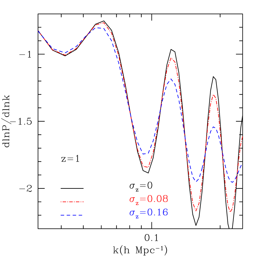
Figure 7: The derivative $d\ln P/d\ln k$ as a function of wavenumber for three different values of the redshift uncertainty. Larger uncertainties cause line-of-sight projections that smear the narrow acoustic oscillations and impede the detectability of cosmological distortions. $\sigma_{z}=0.0$ represents spectroscopic redshift error. $\sigma_{z}=0.08$ and $\sigma_{z}=0.16$ corresponds to $4\%$ and $8\%$ of $\sigma_{z}/(1+z)$ at $z=1$.

4.5 Photometric Redshift Surveys

With the advent of deep wide-field multi-color imaging surveys, it is natural to ask whether photometric redshifts can be used for studies of the acoustic oscillations. In this section, we will study how uncertainties in the galaxy redshifts affect our results. There are two basic lessons. First, recovering the Hubble parameter $H(z)$ requires measuring clustering on fairly small scales along the line of sight, such redshift precision substantially better than 1% is needed. Second, redshift slices selected with photometric redshifts can be sufficiently thin that the acoustic oscillations survive in the angular power spectrum. This means that one can measure $D\!_{A}(z)$ with these surveys, albeit with worse precision per unit survey sky coverage. Hence, photometric redshift surveys lose the advantage of the acoustic oscillations to measure $H(z)$ directly but could measure $D\!_{A}(z)$ if one has a large enough survey. The idea of using transverse clustering to probe dark energy was analyzed in the weak lensing context by Cooray, Hu, Huterer, & Joffre (2001).

When redshifts are uncertain, one is smearing together clustering at multiple distances along the line of sight. Our first task is to consider whether the acoustic oscillations, being narrow features in Fourier space, can survive this projection. The controlling effect is the variation in the comoving angular diameter distance across the range of redshift uncertainty. This can be addressed with Limber’s equation (Limber, 1953; Baugh & Efstathiou, 1994). We model the redshift distribution as a Gaussian of width $\sigma_{z}$ and consider the effects on the angular power spectrum. This is shown in Figure 7, where we plot the derivative $d\ln P/d\ln k$ that controls the measurement of cosmological distortions for 3 different values of $\sigma_{z}$. We adopt a $z=1$ slice and consider 0%, 4%, and 8% uncertainties (1–$\sigma$) in $1+z$. One can see that the oscillation pattern is essentially intact at 4% but substantially degraded at 8%. In detail, we estimate that the errors on $D\!_{A}(z)$ would be increased by 13% for the 4% case and 54% for the 8% case. The effects at $z=3$ are slightly more forgiving, despite the higher $k_{\rm max}$ and hence narrower features, because the derivative of $D\!_{A}(z)$ versus $z$ is slightly less. We therefore conclude that photometric redshift errors of 4% in $1+z$ (1–$\sigma$) are sufficient to preserve the acoustic oscillations for the measurement of $D\!_{A}(z)$ at $z\gtrsim 0.5$.

Having found that the transverse power spectrum is not affected by reasonable projections, we next include the redshift uncertainty in our Fisher matrix formalism. We do this by retaining the Euclidean approximation, i.e. treating the survey as a box of fixed $D_{A}$ and $H$, but smearing the radial position by a Gaussian uncertainty. If the line-of-sight comoving position $r_{z}$ is convolved with an uncertainty of the form $\exp[-(\Delta r_{z})^{2}/2\sigma_{r}^{2}]$ with an uncertainty $\sigma_{r}$, then the Fourier transform of the density field will simply be diminished by the transform of this kernal: $\delta_{\vec{k}}\propto\exp(-k_{\parallel}^{2}\sigma_{r}^{2}/2)$. The observed power spectrum is then (L. Hui, private communication)

$$P(\vec{k})=P_{\rm obs}(\vec{k})e^{-k_{\parallel}^{2}\sigma_{r}^{2}}$$ (18)

where $P_{\rm obs}$ was given in equation (14). In other words, the power is strongly suppressed for large $k_{\parallel}$. The positional uncertainty is related to the redshift uncertainty $\sigma_{z}$ by $\sigma_{r}=c\sigma_{z}/H(z)$.

The introduction of this suppression enters the Fisher matrix calculation through its effect on the effective volume. Modes with a relatively large $k_{\parallel}$ will be swamped by shot noise and therefore give no leverage on the power spectrum measurements. Only modes with $k_{\parallel}\sigma_{r}\lesssim 1$ are useful. Much lower shot noise allows one to retain modes of larger $k_{\parallel}$, but one is fighting a Gaussian suppression.

Because the measurement of $H(z)$ depends on modes aligned near the line of sight, the suppressed contribution from modes with large $k_{\parallel}$ increases the error on $H(z)$ significantly. The measurement of $D\!_{A}(z)$ arises from more transverse modes, and modes with $k_{\parallel}=0$ always exist to give some measurement of $D\!_{A}(z)$. However, for large $k$, only a thin slab of modes with $k_{\parallel}\lesssim 1/\sigma_{r}$ remain useful. As the number of modes will scale as $\sigma_{r}^{-1}$, we expect that the errors on $D\!_{A}(z)$ will scale as $\sqrt{\sigma_{r}}$ for $k_{\rm max}\sigma_{r}\gg 1$.

Figure 8: The error on $D\!_{A}(z)$ and $H(z)$ as a function of the line-of-sight positional uncertainty $\sigma_{r}$ for $z=1$ and $z=3$ redshift bins. CMB and SDSS data are included in each redshift bin. $1\%$ of $\sigma_{z}/(1+z)$ corresponds to 34$h^{-1}{{\rm\;Mpc}}$ at $z=1$ and 27$h^{-1}{{\rm\;Mpc}}$ at $z=3$.

Figure 8 shows the fractional errors on $H(z)$ and $D\!_{A}(z)$ as a function of $\sigma_{r}$ for redshift surveys at $z=1.0$ and $z=3$. The errors are constant for small $\sigma_{r}$ and then increase rapidly beyond a characteristic threshold. Performance at $z=3$ degrades at smaller $\sigma_{r}$ than performance at $z=1.0$. This is because of the larger value of $k_{\rm max}$ for $z=3$. An additional small but non-zero effect is that the redshift distortions are smaller at $z=3$ than at $z=1$. Larger distortions increase the power in the radial direction and allow modes with slightly larger $k_{\parallel}$ to survive the shot noise. The errors on $H(z)$ degrade sharply for $\sigma_{r}\gtrsim 10h^{-1}{\rm\;Mpc}$ at $z=1$ and $5h^{-1}{\rm\;Mpc}$ at $z=3$. These correspond to redshift errors $\sigma_{z}$ of 0.006 and 0.007, respectively. In terms of wavelength resolution $\sigma_{\lambda}/\lambda$, these are 0.003 and 0.002. Hence, our general result is that fractional errors of 0.25% in $1+z$ are required to recover $H(z)$.

In Figure 8, the errors on $D\!_{A}(z)$ in both redshift bins increase relatively slowly at $\sigma_{r}\gtrsim 10h^{-1}{\rm\;Mpc}$ and achieve the predicted $\sqrt{\sigma_{r}}$ dependence at large $\sigma_{r}$. Therefore, to calculate $\sigma_{D_{A}}$ with $\sigma_{r}$ bigger than the values appeared in Figure 8, we can use $\sqrt{\sigma_{r}}$ dependence to interpolate (up to the limit of $\sigma_{z}/(1+z)\approx 4\%$). For numerical reasons, we assume redshift error of $1\%$ in photometric redshift. This is too optimistic for a normal photometric redshift, but one can scale to larger uncertainties. For example, a $4\%$ uncertainty would have errors twice as large, which could be compensated by making the survey area 4 times as large. $1\%$ errors in $(1+z)$ correspond to $\sigma_{r}=34h^{-1}{\rm\;Mpc}$ at $z=1$ and $\sigma_{r}=27h^{-1}{\rm\;Mpc}$ at $z=3$.

Figure 9: Elliptical error regions for $w_{0}$ and $w_{1}$ for photometric redshift surveys with $1\%$ of $\sigma_{z}/(1+z)$ ($\sigma_{z}=0.02$ for $z\sim 1$, $\sigma_{z}=0.04$ for $z=3.0$). Left panel: $\rm{\Lambda CDM}$. Right panel: Model 2 ($w=-2/3$). CMB data and all redshift surveys are included in all cases. The survey parameters written inside the parenthesis are for both $z\sim 1$ and $z=3$ bins. V numbers specify the change in the survey volume relative to the baseline; N the change in the number of galaxies. For SDSS, the fiducial survey parameters (V1N1) with spectroscopic redshifts are used. In both figures, V10N50 is nearly the same as V20N20.

Table 10 shows the errors on $D\!_{A}(z)$ and $H(z)$ for different survey conditions. Increasing the survey volume five-fold while keeping the target density fixed (i.e. V5N5) decreases the error by $\sim\sqrt{5}$, as before. Further increases of the survey volume, which are omitted in Table 10, continue to follow the simple trend of $\sqrt{V_{\rm survey}}$. Increasing the number density with fixed $V_{\rm survey}$ is slightly more efficient than the spectroscopic redshift case ($\sigma_{r}=0$) because the exponential suppression of modes with non-zero $k_{\parallel}$ means that there are always modes that benefit from a larger $n$ to achieve $nP\sim 1$.

Table 11 shows the propagated errors on dark energy parameters for $\rm{\Lambda CDM}$. The left panel of Figure 9 shows the corresponding error ellipses. The errors on $w_{0}$ and $w_{1}$ using photometric redshifts increases by a factor of $\sim 2.4$ with the fiducial condition (V1N1) relative to spectroscopic results while $w(z_{\rm pivot})$ is less affected. As shown in Figure 9, this is because the ellipse is more elongated with a relatively little increase in its minor axis compared to left panel of Figure 5. This is due to the increased dominance of $z\sim 1$ survey over $z=3$. $z_{\rm pivot}$ increases slightly with photometric redshift data. As shown in Figure 3, $D\!_{A}(z)$ at higher $z$ contributes more to the information compared to $H(z)$. Thus, eliminating $H(z)$ by using photometric redshifts will weight higher redshifts slightly more.

Table 11 also shows that increasing $V_{\rm survey}$ by a factor of 20 (V20N20) or a factor of 10 with a 5-fold increase in target density $n$ (V10N50) allows the results from photometric redshift surveys to achieve the accuracy of the spectroscopic redshift surveys. This corresponds to 10 or 20 thousand square degrees of sky at $z=1$ (with 1% errors in $1+z$). Observationally, increasing the number density by 5 times (V10N50) will be more difficult than doubling the survey area because the galaxy luminosity function flattens out around this number density, so that $\sqrt{2}$ in depth is far less than a factor of 5 in source counts. The errors of $w_{0}$ and $w_{1}$ do not scale trivially with $\sqrt{V_{\rm survey}}$ because the SDSS and CMB survey parameters are being held fixed.

Results including the SNe survey data are shown in Table 12. With SNe, improving the redshift survey condition to between V5N5 and V10N10 allows the photometric redshift survey to recover the spectroscopic result in Table 5. This is equivalent to an imaging survey of about 30,000 square degrees with $4\%$ photometric redshift error at $z\sim 1$ and a depth to reach 1000 $z\sim 1$ galaxies per square degree. Surveys such as Pan-STARRS (http://pan-starrs.ifa.hawaii.edu) or the Large Synoptic Survey Telescope (http://www.lssto.org) could achieve this.

Table 13 and Table 14 show the same analysis as Table 11 and 12, but for Model 2 ($w=-2/3$) instead of $\rm{\Lambda CDM}$. The degradation of performance relative to the spectroscopic case is similar. Like the $\rm{\Lambda CDM}$ case, V10N50 or V20N20 recovers the spectroscopic result without SNe, and V5N5 or V10N10 does the job with SNe. The right panel of Figure 9 shows the corresponding error ellipses.

Therefore, after considering both the projection and power suppression effects of redshift uncertainties, we expect that, when combined with supernovae data, surveys with 4% errors on $1+z$ and roughly 30 times more volume than our baseline surveys will be equivalent to the spectroscopic surveys. As this is essentially the full sky at $z\sim 1$, improving beyond these levels will require better redshift accuracy.

5 Conclusion

Understanding the acceleration of the Universe is one of the most important problems in both cosmology and fundamental particle physics. Identifying the physical cause, whether dark energy or some alteration to the theory of gravitation, is certain to be a major breakthrough. Precision measurements of the expansion history of the universe could be crucial in choosing between alternative theories. In this paper, we demonstrated that a standard ruler test using baryonic acoustic oscillations imprinted in the large scale structure could be a superb probe of the acceleration history. The oscillations in the galaxy power spectrum are expected to be robust against contamination from clustering bias, redshift distortions, and other broadband systematic errors.

We have studied the performance that could be achieved on dark energy models from the measurement of the acoustic oscillations in large galaxy spectroscopic surveys at redshifts 0.3, 1, and 3. The $z\sim 1$ baseline survey uses 900,000 galaxies to probe $1.7h^{-3}{\rm\;Gpc}^{3}$; the $z=3$ survey uses a half million galaxies to cover $0.5h^{-3}{\rm\;Gpc}^{3}$. While these numbers are large, the number densities are not, which means that relatively bright galaxies could be used. Using a Fisher matrix treatment of the statistical errors that result from the three-dimensional power spectra, as well as CMB and SNe data, we forecasted errors on the distances along and across the line of sight and then projected these measurements of $H(z)$ and $D\!_{A}(z)$ onto dark energy parameters. Of course, the cosmographical performance are independent of the details of the dark energy model. We summarize our major results below.

First, we have shown that (1–$\sigma$) errors of 0.037 on $\Omega_{X}$, 0.10 on $w(z=0.8)$, and 0.28 on $dw/dz$ are achievable for $\rm{\Lambda CDM}$ when CMB provides the scale of the baryonic oscillations. The constraints on $dw/dz$ are comparable to those from the luminosity distances of future SNe data. Most of constraints were contributed by information in the higher redshift surveys ($z\gtrsim 0.6$) because the baryonic oscillations in the power spectrum are better preserved against nonlinearity at higher redshift. When we combined the redshift survey data with the SNe data, the constraints were improved to 0.16 on $dw/dz$.

Second, we found that fiducial dark energy models with less negative $w$ than $\rm{\Lambda CDM}$ improve overall performance and also favor the galaxy redshift surveys relative to the SNe data. Together, a 0.05 measurement of $dw/dz$ is achieved!

Third, we discussed how the quality of constraints depends upon the the survey volume and number density. Increasing the survey volume with the number density fixed always gives the better result by $\sqrt{V_{\rm survey}}$. Increasing the number density, that is, going deeper with the volume fixed, will also improve the constraints but with asymptotic saturation. Changing the survey volume with a fixed total number of objects has a maximum in performance that is close to the baseline values.

Forth, we computed how well an imaging survey with photometric redshifts could measure the acoustic oscillations. We find that errors of 0.25% in $1+z$ are necessary to retain information on the Hubble parameter $H(z)$. However, redshift errors of 4% in $1+z$ can be tolerated without losing the oscillations to projection effects, and the angular diameter distance could be measured as a function of redshift. We estimate that a survey 20 times larger than our baseline but with 1% redshift error on $1+z$ is needed to replace the spectroscopy, but that the requirement drops to 5–10 times larger when combined with the constraints from SNe. 4% redshift errors require four times more volume.

To date, much of the attention in cosmological probes of acceleration has rightly been given to the studies of distant supernovae. The acoustic oscillations in the galaxy power spectrum have not even been conclusively detected yet. Nevertheless, we are encouraged by the result that the study of acoustic oscillations in large galaxy surveys can achieve comparable performance to upcoming SNe data sets. Given the mystery and importance of the acceleration of the universe, it is crucial to have multiple experiments with independent systematic errors. Moreover, the ability to measure $H(z)$ directly and to probe the expansion at higher redshifts ($z\approx 3$) opens the possibility of detecting new surprises. Although the cosmological constant model is most easily probed at lower redshifts, given the woeful history of theoretical predictions for dark energy, it seems to us unwise to design experiments based too closely on the assumptions of $\rm{\Lambda CDM}$.

While the required redshift surveys are large, they are feasible within the current decade. 8-meter ground based telescopes are sufficiently sensitive, but currently lack the necessary highly multiplexed wide-field spectroscopic capability. Instruments such as the KAOS concept (http://www.noao.edu/kaos) could perform these surveys in about a year of observing. The surveys would of course have many other science applications, both for the study of galaxy evolution and for the search for more speculative features of the linear perturbations, e.g. primordial non-Gaussianity or additional preferred scales. At $z=3$, the reach into the linear regime on intermediate scales exceeds even that of the CMB. Hence, we conclude that such surveys are attractive options for the study of large-scale structure over the next decade.

Table 1: Baseline Survey Parameters

Survey	$z$	$k_{\rm max}$	$V_{\rm survey}\tablenotemark{a}$	$N_{\rm gal}\tablenotemark{b}$	bias	$P(0.2h{\rm\;Mpc^{-1}})\tablenotemark{d}$	$P(k_{\rm max})$	$nP(0.2h{\rm\;Mpc^{-1}})$	$nP(k_{\rm max})$
		$(h{\rm\;Mpc^{-1}})$	($h^{-3}{\rm\;Gpc}^{3})$	$(10^{5})$		$h^{-3}{\rm\;Mpc}^{3}$	$h^{-3}{\rm\;Mpc}^{3}$
SDSS	0.3	0.11	1.0	1.0	2.13		22900		2.29
$z\sim 1$	0.6	0.15	0.29	1.44	1.25		4660		2.33
	0.8	0.17	0.40	2.00	1.40		3590		1.80
	1.0	0.19	0.49	2.46	1.55		3090		1.55
	1.2	0.21	0.56	2.82	1.70	2860	2620	1.43	1.31
$z=3$	3.0	0.53	0.50	5.0	3.30	2950	430	2.95	0.43

Table 2: Dark Energy Models

Model	$w_{0}$	$w_{1}$
1 ($\Lambda$CDM)	$-1$	0
2	$-2/3$	0
3	$-2/3$	$1/6\tablenotemark{b}$
4	$-1$	$1/3\tablenotemark{b}$
5	$-4/3$	$1/3\tablenotemark{b}$
6	$-1.15$	$1/3\tablenotemark{b}$

Table 3: Marginalized Errors on $D\!_{A}(z)$ and $H(z)$ for $\rm{\Lambda CDM}$

Redshift	0.3	0.6	0.8	1.0	1.2	3	1000
$D\!_{A}(z)$ (%)	5.19	4.30	3.22	2.30	2.03	1.19	0.219
$H(z)$ (%)	5.80	5.19	3.59	2.84	2.53	1.48

Note. — The fractional percentage errors (1–$\sigma$) on cosmological distances from the combination of CMB, SDSS, and our standard surveys at $z\sim 1$ and $z=3$.

Table 4: Correlation Matrix for Distance Measurements in $\rm{\Lambda CDM}$

	z	CMB	0.3		0.6		0.8		1.0		1.2		3.0
z		$D_{A}\,$	$D_{A}\,$	$hzz$	$D_{A}\,$	$H\,$	$D_{A}\,$	$H\,$	$D_{A}\,$	$H\,$	$D_{A}\,$	$H\,$	$D_{A}\,$	$H\,$
	$\sqrt{D_{ii}}$	0.002	0.052	0.058	0.043	0.052	0.032	0.036	0.023	0.028	0.020	0.025	0.012	0.015
CMB	$D_{A}\,$	1.000	0.040	$-$0.048	0.054	$-$0.045	0.061	$-$0.064	0.103	$-$0.087	0.123	$-$0.100	0.233	$-$0.192
0.3	$D_{A}\,$	0.040	1.000	$-$0.256	0.002	$-$0.002	0.003	$-$0.003	0.005	$-$0.004	0.006	$-$0.005	0.011	$-$0.009
	$H\,$	$-$0.048	$-$0.256	1.000	$-$0.003	0.003	$-$0.003	0.004	$-$0.006	0.005	$-$0.007	0.006	$-$0.013	0.011
0.6	$D_{A}\,$	0.054	0.002	$-$0.003	1.000	$-$0.255	0.004	$-$0.004	0.006	$-$0.005	0.008	$-$0.006	0.015	$-$0.012
	$H\,$	$-$0.045	$-$0.002	0.003	$-$0.255	1.000	$-$0.003	0.003	$-$0.005	0.005	$-$0.006	0.005	$-$0.012	0.010
0.8	$D_{A}\,$	0.061	0.003	$-$0.003	0.004	$-$0.003	1.000	$-$0.304	0.007	$-$0.006	0.009	$-$0.007	0.016	$-$0.013
	$H\,$	$-$0.064	$-$0.003	0.004	$-$0.004	0.003	$-$0.304	1.000	$-$0.008	0.006	$-$0.009	0.007	$-$0.017	0.014
1.0	$D_{A}\,$	0.103	0.005	$-$0.006	0.006	$-$0.005	0.007	$-$0.008	1.000	$-$0.124	0.015	$-$0.012	0.028	$-$0.023
	$H\,$	$-$0.087	$-$0.004	0.005	$-$0.005	0.005	$-$0.006	0.006	$-$0.124	1.000	$-$0.012	0.010	$-$0.024	0.020
1.2	$D_{A}\,$	0.123	0.006	$-$0.007	0.008	$-$0.006	0.009	$-$0.009	0.015	$-$0.012	1.000	$-$0.120	0.033	$-$0.028
	$H\,$	$-$0.100	$-$0.005	0.006	$-$0.006	0.005	$-$0.007	0.007	$-$0.012	0.010	$-$0.120	1.000	$-$0.027	0.023
3.0	$D_{A}\,$	0.233	0.011	$-$0.013	0.015	$-$0.012	0.016	$-$0.017	0.028	$-$0.024	0.033	$-$0.027	1.000	$-$0.203
	$H\,$	$-$0.192	$-$0.009	0.011	$-$0.012	0.010	$-$0.013	0.014	$-$0.023	0.020	$-$0.028	0.023	$-$0.203	1.000

Note. — All terms are normalized by diagonal terms given in the first row: $a^{\prime}_{ij}=\frac{a_{ij}}{\sqrt{a_{ii}a_{jj}}}$

Table 5: Marginalized Errors on Dark Energy Parameters for $\Lambda$CDM

$z\sim 1$	$z=3$	SNe	$\sigma_{\Omega_{m}\;h^{2}}$/$\Omega_{m}\;h^{2}$	$\sigma_{\Omega_{x}}$	$\sigma_{w_{0}}$	$\sigma_{w_{1}}$	$z_{\rm pivot}$	$\sigma_{w_{zpivot}}$
			0.0094	0.0926	0.882	1.172	0.729	0.218
$\surd$			0.0090	0.0378	0.281	0.353	0.735	0.107
	$\surd$		0.0086	0.0758	0.466	0.446	0.959	0.184
$\surd$	$\surd$		0.0083	0.0368	0.245	0.280	0.796	0.102
		$\surd$	0.0093	0.0088	0.116	0.231	0.478	0.035
$\surd$		$\surd$	0.0088	0.0083	0.093	0.183	0.471	0.033
	$\surd$	$\surd$	0.0086	0.0085	0.096	0.189	0.479	0.034
$\surd$	$\surd$	$\surd$	0.0082	0.0082	0.083	0.161	0.476	0.032

Note. — Check marks indicate the data sets being used; CMB and SDSS data are included in all sets. The fiducial redshift survey parameters (V1N1) are used. $z_{\rm pivot}$ is the redshift at which the errors on the value of $w(z)$ is independent from the slope $w_{1}$. $\sigma(w_{zpivot})$ is the error on the value of $w$ at that redshift; this is also the error on $w$ that would be found if $w_{1}$ were held fixed at the fiducial value. All errors are 1–$\sigma$.

Table 6: Cosmological Errors from Different Fiducial Dark Energy Models

Model	$z\sim 1$	$z=3$	SNe	$\sigma_{\Omega_{m}\;h^{2}}$/$\Omega_{m}\;h^{2}$	$\sigma_{\Omega_{x}}$	$\sigma_{w_{0}}$	$\sigma_{w_{1}}$	$z_{\rm pivot}$	$\sigma_{w_{zpivot}}$
Model 2	$\surd$			0.0090	0.0259	0.129	0.092	1.249	0.057
		$\surd$		0.0088	0.0485	0.247	0.158	1.484	0.078
	$\surd$	$\surd$		0.0085	0.0245	0.119	0.081	1.333	0.050
			$\surd$	0.0094	0.0134	0.087	0.122	0.682	0.023
	$\surd$		$\surd$	0.0090	0.0088	0.049	0.062	0.714	0.022
		$\surd$	$\surd$	0.0087	0.0097	0.056	0.072	0.713	0.023
	$\surd$	$\surd$	$\surd$	0.0084	0.0083	0.045	0.052	0.744	0.022
Model 3	$\surd$			0.0090	0.0266	0.131	0.097	1.306	0.033
		$\surd$		0.0088	0.0530	0.268	0.190	1.389	0.043
	$\surd$	$\surd$		0.0085	0.0256	0.124	0.089	1.351	0.028
			$\surd$	0.0094	0.0158	0.081	0.107	0.741	0.019
	$\surd$		$\surd$	0.0090	0.0092	0.045	0.049	0.853	0.017
		$\surd$	$\surd$	0.0087	0.0103	0.051	0.058	0.821	0.018
	$\surd$	$\surd$	$\surd$	0.0085	0.0086	0.042	0.042	0.906	0.016
Model 4	$\surd$			0.0090	0.0320	0.180	0.144	1.203	0.049
		$\surd$		0.0088	0.0653	0.367	0.275	1.314	0.065
	$\surd$	$\surd$		0.0085	0.0313	0.171	0.132	1.259	0.043
			$\surd$	0.0094	0.0127	0.106	0.142	0.729	0.022
	$\surd$		$\surd$	0.0090	0.0090	0.062	0.075	0.774	0.021
		$\surd$	$\surd$	0.0087	0.0098	0.070	0.087	0.764	0.022
	$\surd$	$\surd$	$\surd$	0.0085	0.0086	0.056	0.064	0.803	0.021
Model 5	$\surd$			0.0090	0.0454	0.353	0.429	0.773	0.122
		$\surd$		0.0086	0.0844	0.560	0.547	0.968	0.183
	$\surd$	$\surd$		0.0083	0.0443	0.312	0.344	0.846	0.113
			$\surd$	0.0094	0.0089	0.132	0.258	0.488	0.040
	$\surd$		$\surd$	0.0089	0.0085	0.106	0.206	0.480	0.038
		$\surd$	$\surd$	0.0086	0.0087	0.109	0.208	0.491	0.038
	$\surd$	$\surd$	$\surd$	0.0083	0.0084	0.095	0.179	0.487	0.037
Model 6	$\surd$			0.0090	0.0368	0.240	0.232	0.975	0.078
		$\surd$		0.0087	0.0766	0.463	0.386	1.166	0.107
	$\surd$	$\surd$		0.0084	0.0365	0.224	0.201	1.057	0.070
			$\surd$	0.0094	0.0101	0.119	0.190	0.604	0.029
	$\surd$		$\surd$	0.0090	0.0086	0.081	0.125	0.609	0.029
		$\surd$	$\surd$	0.0087	0.0090	0.087	0.133	0.619	0.028
	$\surd$	$\surd$	$\surd$	0.0084	0.0084	0.071	0.105	0.626	0.028

Note. — Check marks indicate the data sets being used; CMB and SDSS data are included in all sets. The fiducial redshift survey parameters (V1N1) are used.

Table 7: Marginalized Errors on $D\!_{A}(z)$ and $H(z)$ as a Function of Survey Parameters

Surveys			Redshift
$z\sim 1$	$z=3$		0.3	0.6	0.8	1.0	1.2	3.0
V1N1	V1N1	$D\!_{A}(z)$	5.19	4.30	3.22	2.30	2.03	1.19
		$H(z)$	5.80	5.19	3.59	2.84	2.53	1.48
V1N5	V1N5	$D\!_{A}(z)$	5.19	3.50	2.57	1.74	1.52	0.88
		$H(z)$	5.80	4.44	3.00	2.30	2.01	1.08
V5N1	V5N1	$D\!_{A}(z)$	5.19	3.52	2.75	2.12	1.91	1.10
		$H(z)$	5.80	3.83	2.79	2.32	2.13	1.33
V5N5	V5N5	$D\!_{A}(z)$	5.19	1.93	1.45	1.04	0.93	0.57
		$H(z)$	5.80	2.33	1.62	1.28	1.15	0.69

Note. — 1–$\sigma$ fractional percentage errors on cosmological distances. CMB and SDSS are included in all sets. For SDSS, the fiducial condition (V1N1) is always used. V1N1 means the fiducial condition described in Table 1. V5N1: 5 times larger survey volume with 5 times smaller number density. V1N5: 5 times higher number of objects with the standard survey volume, i.e. 5 times higher number density. V5N5: 5 times more survey volume with the standard number density.

Table 8: Marginalized errors for $\Lambda$CDM for Various Survey Sizes

$z\sim 1$	$z=3$	$\sigma_{\Omega_{m}\;h^{2}}$/$\Omega_{m}\;h^{2}$	$\sigma_{\Omega_{x}}$	$\sigma_{w_{0}}$	$\sigma_{w_{1}}$	$z_{\rm pivot}$	$\sigma_{w_{zpivot}}$
V1N1		0.0090	0.0378	0.281	0.353	0.735	0.107
V5N5		0.0079	0.0195	0.142	0.191	0.680	0.056
	V1N1	0.0086	0.0758	0.466	0.446	0.959	0.184
	V5N5	0.0070	0.0724	0.399	0.306	1.239	0.126
V1N1	V1N1	0.0083	0.0368	0.245	0.280	0.796	0.102
V1N1	V5N5	0.0069	0.0358	0.210	0.199	0.961	0.088
V5N5	V1N1	0.0074	0.0192	0.135	0.176	0.699	0.055
V5N5	V5N5	0.0064	0.0186	0.120	0.142	0.762	0.053

Note. — Left two columns indicate how the sizes of the $z\sim 1$ and $z=3$ surveys are being varied; blanks mean that the survey is excluded. CMB and SDSS are included in all rows. For SDSS, the fiducial parameters (V1N1) are always used.

Table 9: Marginalized Errors on $D\!_{A}(z)$ and $H(z)$ with Negligible $\beta$ for Different Baryon Fractions

$\Omega_{b}$		Redshift
		0.3	0.6	0.8	1.0	1.2	3.0
0.005	$D\!_{A}(z)$	13.03	15.64	11.47	9.21	7.68	3.16
	$H(z)$	12.71	14.05	10.50	8.49	7.27	3.56
0.05	$D\!_{A}(z)$	5.80	5.66	4.03	2.92	2.59	1.44
	$H(z)$	6.68	7.83	4.75	4.04	3.64	2.03

Note. — 1–$\sigma$ fractional percentage errors on cosmological distances for $\rm{\Lambda CDM}$. CMB and SDSS are included in all sets. The derivatives are computed with $\beta\approx 0$, thereby causing the redshift and cosmological distortions to be more degenerate. The usual $\beta$’s are used to compute $V_{\rm eff}$.

Table 10: Marginalized Errors on $D\!_{A}(z)$ and $H(z)$ for Photometric Redshift Surveys

Surveys			Redshift
$z\sim 1$	$z=3$		0.3	0.6	0.8	1.0	1.2	3.0
V1N1	V1N1	$D\!_{A}(z)$	5.19	6.98	4.84	4.25	3.90	2.26
		$H(z)$	5.80	22.37	19.58	18.28	17.77	16.15
V1N5	V1N5	$D\!_{A}(z)$	5.19	4.84	3.26	2.81	2.56	1.57
		$H(z)$	5.80	16.33	14.29	13.27	12.88	10.11
V5N5	V5N5	$D\!_{A}(z)$	5.19	3.14	2.19	1.93	1.77	1.06
		$H(z)$	5.80	10.02	8.78	8.21	7.99	7.26

Note. — The fractional percentage error on the cosmological distances under conditions appropriate to photometric redshifts. The redshift accuracy has been degraded to 1% (1–$\sigma$) on $\sigma_{z}/(1+z)=\Delta\lambda/\lambda$, i.e. $\sigma_{z}=2\%$ at $z=1$ and 4% at $z=3$. The results will scale as $\sqrt{\sigma_{z}}$, and $\sigma_{z}$ would typically be larger for actual photometric redshifts. The left two columns show variations in the survey parameters. V1N1 is the standard survey volume and number density. V1N5 allows for a 5-fold increase in the number density. V5N5 is 5 times more volume at the standard number density. CMB and SDSS are included in all sets. For SDSS, the fiducial survey parameters (V1N1) are used and spectroscopic redshifts ($\sigma_{z}=0$) are adopted. The $\Lambda$CDM fiducial model is used.

Table 11: Marginalized Errors for $\Lambda$CDM for Photometric Redshift Surveys

$z\sim 1$	$z=3$	$\sigma_{\Omega_{m}\;h^{2}}$/$\Omega_{m}\;h^{2}$	$\sigma_{\Omega_{x}}$	$\sigma_{w_{0}}$	$\sigma_{w_{1}}$	$z_{\rm pivot}$	$\sigma_{w_{zpivot}}$
V1N1		0.0091	0.0799	0.613	0.704	0.834	0.175
V1N5		0.0089	0.0736	0.534	0.578	0.887	0.150
	V1N1	0.0090	0.0859	0.752	0.979	0.735	0.218
	V1N5	0.0089	0.0820	0.670	0.855	0.742	0.217
V1N1	V1N1	0.0088	0.0777	0.584	0.668	0.834	0.175
V1N5	V1N5	0.0085	0.0708	0.504	0.544	0.887	0.148
V5N5	V5N5	0.0077	0.0592	0.413	0.437	0.904	0.118
V10N10	V10N10	0.0069	0.0485	0.335	0.352	0.912	0.094
V10N50	V10N50	0.0062	0.0375	0.256	0.267	0.921	0.071
V20N20	V20N20	0.0060	0.0379	0.261	0.276	0.908	0.073

Note. — Redshift uncertainties have been applied as in Table 10: 1% in $\sigma_{z}/(1+z)$. Various survey sizes are investigated, as detailed in the left two columns. V numbers specify the change in the survey volume; N the change in the number of galaxies. Note that V20 is 20,000 square degrees at $z\sim 1$ and about 3000 square degrees at $z\sim 3$. Blanks indicate that a survey has been excluded. Larger redshift uncertainties can be offset with more volume; for example, 4% errors in $\sigma_{z}/(1+z)$ would require 4 times more volume to produce the results in this Table. CMB and SDSS are included in all rows. For SDSS, the fiducial parameters (V1N1) with spectroscopic redshifts are used in all cases.

Table 12: Marginalized Errors for $\Lambda$CDM for Photometric Redshift Survey with SNe

$z\sim 1$	$z=3$	$\sigma_{\Omega_{m}\;h^{2}}$/$\Omega_{m}\;h^{2}$	$\sigma_{\Omega_{x}}$	$\sigma_{w_{0}}$	$\sigma_{w_{1}}$	$z_{\rm pivot}$	$\sigma_{w_{zpivot}}$
		0.0093	0.0088	0.116	0.231	0.478	0.035
V1N1		0.0089	0.0085	0.106	0.212	0.473	0.034
V1N5		0.0087	0.0083	0.098	0.195	0.470	0.034
	V1N1	0.0090	0.0087	0.114	0.229	0.477	0.034
	V1N5	0.0087	0.0086	0.113	0.227	0.476	0.034
V1N1	V1N1	0.0086	0.0084	0.105	0.211	0.473	0.034
V1N5	V1N5	0.0083	0.0082	0.097	0.193	0.470	0.033
V5N5	V5N5	0.0073	0.0080	0.087	0.171	0.471	0.032
V10N10	V10N10	0.0065	0.0078	0.077	0.148	0.478	0.031
V10N50	V10N50	0.0060	0.0076	0.066	0.119	0.496	0.030
V20N20	V20N20	0.0058	0.0076	0.068	0.124	0.495	0.030

Note. — As Table 11, but the SNe data have also been included.

Table 13: Marginalized Errors for Model 2 for Photometric Redshift Surveys

$z\sim 1$	$z=3$	$\sigma_{\Omega_{m}\;h^{2}}$/$\Omega_{m}\;h^{2}$	$\sigma_{\Omega_{x}}$	$\sigma_{w_{0}}$	$\sigma_{w_{1}}$	$z_{\rm pivot}$	$\sigma_{w_{zpivot}}$
V1N1		0.0091	0.0637	0.395	0.278	1.383	0.087
V1N5		0.0090	0.0563	0.332	0.224	1.452	0.069
	V1N1	0.0092	0.0618	0.342	0.249	1.285	0.122
	V1N5	0.0090	0.0590	0.284	0.187	1.376	0.119
V1N1	V1N1	0.0090	0.0545	0.305	0.207	1.412	0.086
V1N5	V1N5	0.0087	0.0457	0.245	0.160	1.476	0.068
V5N5	V5N5	0.0079	0.0346	0.182	0.118	1.476	0.053
V10N10	V10N10	0.0071	0.0264	0.138	0.090	1.463	0.041
V10N50	V10N50	0.0064	0.0191	0.099	0.065	1.453	0.030
V20N20	V20N20	0.0063	0.0195	0.102	0.067	1.436	0.032

Note. — As Table 11, but fiducial model 2 ($w=-2/3$) has been used.

Table 14: Marginalized Errors for Model 2 for Photometric Redshift Surveys with SNe

$z\sim 1$	$z=3$	$\sigma_{\Omega_{m}\;h^{2}}$/$\Omega_{m}\;h^{2}$	$\sigma_{\Omega_{x}}$	$\sigma_{w_{0}}$	$\sigma_{w_{1}}$	$z_{\rm pivot}$	$\sigma_{w_{zpivot}}$
		0.0094	0.0134	0.087	0.122	0.682	0.023
V1N1		0.0091	0.0104	0.066	0.089	0.695	0.023
V1N5		0.0089	0.0091	0.057	0.072	0.716	0.023
	V1N1	0.0091	0.0120	0.076	0.107	0.678	0.023
	V1N5	0.0089	0.0112	0.068	0.095	0.676	0.023
V1N1	V1N1	0.0088	0.0100	0.062	0.084	0.693	0.023
V1N5	V1N5	0.0086	0.0088	0.053	0.067	0.713	0.023
V5N5	V5N5	0.0077	0.0079	0.046	0.054	0.743	0.022
V10N10	V10N10	0.0070	0.0073	0.041	0.044	0.799	0.021
V10N50	V10N50	0.0063	0.0068	0.037	0.035	0.904	0.019
V20N20	V20N20	0.0062	0.0069	0.038	0.037	0.881	0.020

Note. — As Table 11, but fiducial model 2 ($w=-2/3$) has been used and SNe data is included.

References

- Adelberger et al. (1998) Adelberger, K. L., Steidel, C. C., Giavalisco, M., Dickinson, M., Pettini, M., & Kellogg, M. 1998, ApJ, 505, 18
- Alcock-Paczynski (1979) Alcock, C. & Paczynski, B. 1979, Nature, 281, 358
- Aldering et al. (2002) Aldering, G., et al., 2002, SPIE, 4835, 146 [astro-ph/0209550]
- Armendariz-Picon et al. (2000) Armendariz-Picon, C., Mukhanov, V., & Steinhardt, P.J., 2000, Phys. Rev. Lett., 85, 4438
- Ballinger et al. (1995) Ballinger, W.E., Peacock, J.A., Heavens, A.F., 1996, MNRAS, 282, 877
- Baugh & Efstathiou (1994) Baugh, C.M., & Efstathiou, G. 1994, MNRAS, 267, 323
- Bennett et al. (2003) Bennett, C. et al. 2003, ApJ, in press [astro-ph/0302208]
- Benoît et al. (2003) Benoît, A. et al. 2003, A&A, 399, L19
- de Bernardis et al. (2000) de Bernardis, P., et al., 2000, Nature, 404, 955
- Bilic et al. (2002) Bilic N., Tupper G.B., Viollier R.D., 2002, Phys.Lett. B, 535 17
- Blake & Glazebrook (2003) Blake, C., & Glazebrook, K., 2003, ApJ, submitted [astro-ph/0301632]
- Bond & Efstathiou (1984) Bond, J.R. & Efstathiou, G. 1984, ApJ, 285, L45
- Bond et al. (1997) Bond, J.R., Efstathiou, G., & Tegmark, M., 1997, MNRAS, 291, L33
- Bond & Szalay (1983) Bond, J.R., & Szalay, A. 1983, ApJ, 276, 443
- Boyle et al. (2001) Boyle, L.A., Caldwell, R.R., & Kamionkowski, M., 2002, Phys Lett, B545, 17
- Bucher & Spergel (1999) Bucher, M., & Spergel, D.N., 1999, Phys. Rev. D, 60, 043505
- Caldwell et al. (1998) Caldwell, R.R., Dave, R., & Steinhardt, P.J., 1998, Ap&SS, 261, 303
- Carroll, Press, & Turner (1992) Carroll, S. M., Press, W. H., & Turner, E. L. 1992, ARA&A, 30, 499
- Coles (1993) Coles, P. 1993, MNRAS, 262, 1065
- Coles et al. (1999) Coles, P., Melott, A.L., & Munshi, D., 1999, ApJ, 521, L5
- Cooray & Huterer (1999) Cooray, A., & Huterer, D., 1999, ApJ, 513, 95
- Cooray, Hu, Huterer, & Joffre (2001) Cooray, A., Hu, W., Huterer, D., & Joffre, M. 2001, ApJ, 557, L7
- Deffayet et al. (2002) Deffayet, C., Dvali, G., & Gabadadze, G., 2002, Phys. Rev. D, 65, 044023
- Dekel & Lahav (1999) Dekel, A., & Lahav, O., 1999, ApJ, 520, 24
- Eisenstein & Hu (1998a) Eisenstein, D.J., & Hu, W. 1998a, ApJ, 496, 605
- Eisenstein et al. (1998) Eisenstein, D. J., Hu, W., & Tegmark, M. 1998, ApJ, 504, L57
- Eisenstein et al. (1999) Eisenstein, D. J., Hu, W., & Tegmark, M. 1999, ApJ, 518, 2
- Eisenstein et al. (2001) Eisenstein, D. J. et al. 2001, AJ, 122, 2267
- Eisenstein (2003) Eisenstein, D.J., 2003, in Wide-field Multi-Object Spectroscopy, ASP Conference Series, ed. A. Dey
- Efstathiou et al. (2002) Efstathiou, G., et al., 2002, MNRAS, 330, 29
- Feldman, Kaiser, & Peacock (1994) Feldman, H. A., Kaiser, N., & Peacock, J. A. 1994, ApJ, 426, 23
- Freese & Lewis (2002) Freese K., & Lewis M., 2002, Phys.Lett., B, 540, 1
- Frieman et al. (1995) Frieman, J.A., Hill, C.T., Stebbins, A., & Waga, I., 1995, Phys. Rev. Lett., 75, 2077
- Frieman et al. (2003) Frieman, J.A., Huterer, D., Linder, E.V., & Turner, M.S., 2003, Phys. Rev. D, 67, 083505
- Gawiser & Silk (1998) Gawiser, E. & Silk, J. 1998, Science, 280, 1405
- Gu & Hwang (2001) Gu, J., & Hwang, W., 2001, Phys Lett, B517, 1
- Haiman et al. (2001) Haiman, Z., Mohr, J.J., Holder, G.P., 2001, ApJ, 553, 545
- Hamilton (1998) Hamilton, A.J.S., 1998, “The Evolving Universe”, ed. D. Hamilton (Kluwer: Dordrecht), p. 185; astro-ph/9708102
- Halverson et al. (2002) Halverson, N. W. et al. 2002, ApJ, 568, 38
- Hanany et al. (2000) Hanany, S., et al., 2000, ApJ, 545, L5
- Hatton & Cole (1999) Hatton, S. & Cole, S. 1999, MNRAS, 310, 1137
- Heavens & Taylor (1997) Heavens, A. F. & Taylor, A. N. 1997, MNRAS, 290, 456
- Holtzman (1989) Holtzman, J. A. 1989, ApJS, 71, 1
- Hu & Sugiyama (1996) Hu, W. & Sugiyama, N. 1996, ApJ, 471, 542
- Hu et al. (1998) Hu, W., Eisenstein, D.J., & Tegmark, M. 1998, Phys. Rev. Lett., 80, 5255
- Hu & Haiman (2003) Hu, W. & Haiman, Z. 2003, Phys. Rev. D, in press [astro-ph/0306053]
- Hui et al. (1999) Hui, L., Stebbins, A., & Burles, S., 1999, ApJ, 511, L5
- Huterer & Turner (1999) Huterer, D., & Turner, M.S., 1999, Phys. Rev. D, 60, 1301
- Huterer & Turner (2001) Huterer, D., & Turner, M.S., 2001, Phys. Rev. D, 64, 123527
- Huterer & Starkman (2003) Huterer, D. & Starkman, G., 2003, Phys. Rev. Lett., 90, 031301
- Jain & Bertschinger (1994) Jain, B., & Bertschinger, E., 1994, ApJ, 431, 495
- Jungman et al. (1996) Jungman, G., Kamionkowski, M., Kosowsky, A., & Spergel, D.N., 1996, Phys. Rev. D, 54, 1332
- Kaiser (1986) Kaiser, N. 1986, MNRAS, 219, 785
- Kaiser (1987) Kaiser, N. 1987, MNRAS, 227, 1
- Kasuya (2001) Kasuya, S., 2001, Phys Lett, B515, 121
- Knox (1995) Knox, L., 1995, Phys. Rev. D, 52, 4307
- Kujat et al. (2002) Kujat, J., Linn, A.M., Scherrer, R.J., & Weinberg, D.H., 2002, ApJ, 572, 1
- Lange et al. (2001) Lange, A.E., et al. 2001, Phys. Rev. D, 63, 2001
- Limber (1953) Limber, D.N. 1953, ApJ, 117, 134
- Linder (2003) Linder, E.V., 2003, Phys. Rev. Lett., 90, 1301
- Linder (2003) Linder, E.V., 2003, Phys. Rev. D, submitted [astro-ph/0304001]
- Linder & Huterer (2003) Linder, E.V., & Huterer, D., 2003, Phys. Rev. D, 67, 081303
- Maor, Brustein, & Steinhardt (2001) Maor, I., Brustein, R., & Steinhardt, P. J. 2001, Phys. Rev. Lett., 86, 6
- Maor, Brustein, McMahon, & Steinhardt (2002) Maor, I., Brustein, R., McMahon, J., & Steinhardt, P. J. 2002, Phys. Rev. D, 65, 123003
- Matsubara & Szalay (2002) Matsubara, T., & Szalay, A.S., 2002, ApJ, 574, 1
- Matsubara & Szalay (2003) Matsubara, T. & Szalay, A. S. 2003, Phys. Rev. Lett., 90, 21302
- Meiksin, White, & Peacock (1999) Meiksin, A., White, M., & Peacock, J. A. 1999, MNRAS, 304, 851
- Meiksin & White (1999) Meiksin, A., & White, M., 1999, MNRAS, 308, 1179
- Miller et al. (1999) Miller, A.D., Caldwell, R., Devlin, M.J., Dorwart, W.B., Herbig, T., Nolta, M.R., Page, L.A., Puchalla, J., Torbet, E., & Tran, H.T., 1999, ApJ, 524, L1
- Miller et al. (2001) Miller, C., Nichol, R.C., & Batuski, D.J., 2001, ApJ, 555, 68
- Newman & Davis (2000) Newman, J.A., & Davis, M., 2000, ApJ, 534, L11
- Newman et al. (2002) Newman, J.A., Marinoni, C., Coil, A.L., & Davis, M., 2002, PASP, 114, 29
- Peebles & Yu (1970) Peebles, P. J. E. & Yu, J. T. 1970, ApJ, 162, 815
- Perlmutter et al. (1999) Perlmutter, S. et al. 1999, ApJ, 517, 565
- Percival et al. (2001) Percival, W., et al., 2001, MNRAS, 327, 1297
- Popa et al. (2001) Popa, L.A., Burigana, C., Mandolesi, N., 2001, ApJ, 558, 10
- Ratra & Peebles (1988) Ratra, B. & Peebles, P.J.E., 1988, Phys. Rev. D, 37, 3406
- Riess et al. (1998) Riess, A. G. et al. 1998, AJ, 116, 1009
- Riess et al. (2001) Riess, A.G., et al., 2001 ApJ, 560, 49
- Scherrer & Weinberg (1998) Scherrer, R.J., & Weinberg, D.H. 1998, ApJ, 504, 607
- Scott, Silk, & White (1995) Scott, D., Silk, J., & White, M. 1995, Science, 268, 829
- Seljak (2000) Seljak, U., 2000, MNRAS, 318, 203
- Spergel et al. (2003) Spergel, D.N.S., et al., 2003, ApJ, in press [astro-ph/0302209]
- Steidel et al. (1996) Steidel, C.C., Giavalisco, M., Pettini, M., Dickinson, M., & Adelberger, K.L., 1996, ApJ, 462, L17
- Steidel et al. (1998) Steidel, C. C., Adelberger, K. L., Dickinson, M., Giavalisco, M., Pettini, M., & Kellogg, M. 1998, ApJ, 492, 428
- Steinhardt (1997) Steinhardt, P.J., 1997, in Critical Dialogues in Cosmology, ed. N. Turok (World Scientific)
- Taylor & Watts (2001) Taylor, A. N. & Watts, P. I. R. 2001, MNRAS, 328, 1027
- Tegmark (1997) Tegmark, M. 1997, Phys. Rev. Lett., 79, 3806
- Tegmark, Taylor, & Heavens (1997) Tegmark, M., Taylor, A. N., & Heavens, A. F. 1997, ApJ, 480, 22
- Tegmark, Eisenstein, Hu, & de Oliveira-Costa (2000) Tegmark, M., Eisenstein, D. J., Hu, W., & de Oliveira-Costa, A. 2000, ApJ, 530, 133
- Tegmark (2001) Tegmark, M., 2001, Phys. Rev. D, 66, 103507
- Tegmark et al. (2001) Tegmark, M., Zaldarriaga, M., & Hamilton, A.J., 2001, Phys. Rev. D, 63, 3007
- Tonry et al. (2003) Tonry, J.L., et al., 2003, ApJ, in press [astro-ph/0305008]
- Turner & White (1997) Turner, M. S. & White, M. 1997, Phys. Rev. D, 56, 443
- Wang & Garnavich (2001) Wang, Y., & Garnavich, P.M., 2001, ApJ, 552, 445
- Wang, Spergel, & Strauss (1999) Wang, Y., Spergel, D. N., & Strauss, M. A. 1999, AIP Conf. Proc. 478: COSMO-98, 164
- Weller & Albrecht (2002) Weller, J., & Albrecht, A., 2002, Phys. Rev. D, 65, 103512
- York et al. (2000) York, D.G., et al. 2000, AJ, 120, 1579
- Zaldarriaga et al. (1997) Zaldarriaga, M., Spergel, D.N., & Seljak, U., 1997, ApJ, 488, 1
- Zlatev et al. (1999) Zlatev, I., Wang, L., & Steinhardt, P.J., 1999, Phys. Rev. Lett., 82, 896