The End of the MACHO Era:
Limits on Halo Dark Matter From Stellar Halo Wide Binaries

Abstract

We simulate the evolution of halo wide binaries in the presence of the MAssive Compact Halo Objects (MACHOs) and compare our results to the sample of wide binaries of Chanamé & Gould (2003). The observed distribution is well fit by a single power law for angular separations, $3.\!\!\arcsec 5<\Delta\theta<900\arcsec$, whereas the simulated distributions show a break in the power law whose location depends on the MACHO mass and density. This allows us to place upper limits on the MACHO density as a function of their assumed mass. At the 95% confidence level, we exclude MACHOs with masses $M>43{\rm\ M_{\odot}}$ at the standard local halo density $\rho_{H}$. This all but removes the last permitted window for a full MACHO halo for masses $M>10^{-7.5}{\rm\ M_{\odot}}$.

1. Introduction

After formation, wide binaries retain their original orbital parameters except in so far as they are affected by gravitational encounters, or either one or both binary members evolve off the main sequence. These systems can therefore be used to probe inhomogeneities of Galactic potential that may be due to black holes, low luminosity stars, molecular clouds, or other objects, because their low binding energies are easily overcome by gravitational perturbations (Heggie, 1975).

Bahcall, Hut & Tremaine (1985) were the first to apply this principle, using wide binaries in the Galactic disk to investigate disk dark matter in the Solar neighborhood. Weinberg, Shapiro & Wasserman (1987) refined this approach by incorporating several effects that were previously ignored. In particular, they showed that gravitational encounters do not in general induce a sharp cutoff in the binary semi-major axis distribution, but rather generate a break in its power law. Although there have been extensive investigations of disk binary systems, they have not yielded strong conclusions about the disk potential. This is partly due to the relatively small size of the disk binary samples available, partly to the fact that they do not have good sensitivity for separations $\gtrsim 0.1$ pc, and partly because of the intrinsic complexity of the disk potential. In principle, halo binaries could be used to search for dark matter, but this has never been done, primarily because there were no halo-binary samples adequate to the task.

However, halo dark matter has been investigated by several other techniques. Lacey & Ostriker (1985) suggested a mechanism for disk heating by supermassive black holes and discussed that black holes with $M>10^{6}{\rm\ M_{\odot}}$ could destroy the disk. Null results of a search for “echoes” of gamma-ray bursts induced by gravitational lensing constrained halo dark matter in the mass range $M\sim 10^{6.5}-10^{8.5}{\rm\ M_{\odot}}$ (Nemiroff et al., 1993). Moore (1993) argued that massive black holes $M>10^{3}{\rm\ M_{\odot}}$ could disrupt low-mass globular clusters, which would imply an upper limit $M<10^{3}{\rm\ M_{\odot}}$. However, this argument is somewhat sensitive to assumptions about the initial population of globular clusters. Finally, microlensing experiments by the MACHO collaboration (Alcock et al., 2001), the EROS collaboration (Afonso et al., 2003), and the two collaborations working together (Alcock et al., 1998) found that MAssive Compact Halo Objects (MACHOs) with $10^{-7.5}{\rm\ M_{\odot}}<M<30{\rm\ M_{\odot}}$ cannot account for the mass of the dark halo. De Rújula, Jetzer & Massó (1992) argued that baryonic dark matter with $M<10^{-7}{\rm\ M_{\odot}}$ would have evaporated away in a Galactic time scale.

The publication of the $\mu>0.\!\!\arcsec 18{\rm\ yr^{-1}}$ proper motion limited New Luyten Two Tenths (NLTT) catalog (Luyten, 1979; Luyten & Hughes, 1980) has vastly increased the pool of available data on binary systems, but the short color baseline of the photographic photometry in NLTT rendered halo/disk discrimination extremely difficult. However, Gould & Salim (2003) and Salim & Gould (2003) revised NLTT (rNLTT) with improved astrometry and photometry for the 44% of the sky covered by the intersection of the Second Incremental Release of the Two Micron All Sky Survey and the first Palomar Observatory Sky Survey. Chanamé & Gould (2003, hereafter CG) then constructed a homogeneous catalog of binaries from rNLTT and classified each entry as either disk or halo.

In this paper, we use Monte Carlo simulations to evaluate the effect of MACHOs on the halo binary distribution and compare these predictions with the observed halo binary sample of CG by means of a likelihood analysis. We briefly describe our CG halo binary sample in § 2 and make simple analytic estimates of the effects of perturbers in § 3. Detailed justifications of our assumptions and our Monte Carlo algorithm are presented in § 4. We present the results of our numerical simulations in § 5 and the likelihoods of halo dark-matter models in § 6. Finally, we summarize our results in § 7.

2. The CG Halo Wide Binaries

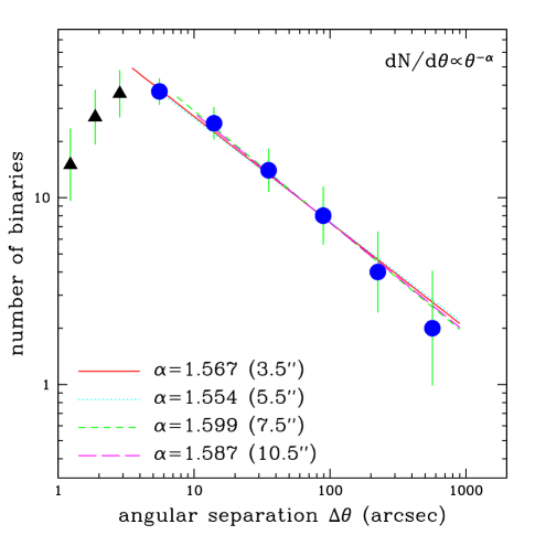
Figure 1.— Halo binary distribution function from the catalog of Chanamé & Gould (2003). Samples of wide binary systems are complete up to 900″ while the lower limit in angular separation is not precisely established. The circles represent actual counts in six equal logarithmic bins over $3.\!\!\arcsec 5\leq\Delta\theta<900\arcsec$. The triangles show three $1\arcsec$ bins for $\Delta\theta<3.\!\!\arcsec 5$ and are rescaled to account for the smaller bin sizes relative to the circles. Various lines represent fits for subsamples with different lower limits in angular separation. Error bars represent one standard deviation $\sigma=n^{-1/2}/\ln 10$.

Figure 1 shows the halo binaries from the CG catalog upon which the current work is based. This binary distribution function is well approximated by a single power law from $\Delta\theta=3.\!\!\arcsec 5$ to the catalog limit at $\Delta\theta=900\arcsec$. However, since the lower threshold of completeness is not precisely established, we consider several different lower limits. There are respectively (90, 68, 59, 47) binaries in the samples with lower limits ($3.\!\!\arcsec 5$, $5.\!\!\arcsec 5$, $7.\!\!\arcsec 5$, $10.\!\!\arcsec 5$). For $\Delta\theta\lesssim 3.\!\!\arcsec 5$, the sample is not complete, and the deviation from a power-law distribution is clearly shown as triangles in Figure 1. However, since the fit is insensitive to the choice of lower limit ($\Delta\theta\geq 3.\!\!\arcsec 5$), we adopt a lower threshold of $\Delta\theta=3.\!\!\arcsec 5$. Since severe incompleteness clearly sets in at $\Delta\theta<3.\!\!\arcsec 5$, one might be concerned about more modest incompleteness just above our adopted boundary $\Delta\theta=3.\!\!\arcsec 5$. However, as we discuss in § 6, incompleteness near $\Delta\theta\sim 3.\!\!\arcsec 5$ would act to lessen the likelihood difference between a halo dark-matter model and the observations. Therefore, our procedure is conservative.

Assuming that the initial binary distribution is characterized by a power law, the slope of which might be different from the final observed one, the observed binary distribution can yield significant constraints on halo dark matter. Since binary systems with large semi-major axes, $a\gtrsim 0.1$ pc, are more liable to be disturbed by perturbers than those with small $a$, the deviation (or lack thereof) from a power-law distribution at wide angular separations provides a test of halo dark-matter models.

3. Theoretical Expectations

We begin by considering two extreme regimes; the tidal regime ($b_{\rm min}\gg a$) and the Coulomb regime ($b_{\rm min}\ll a$), where $a$ is the binary semi-major axis and,

$$b_{\rm min} = \left({M\over\pi\rho vT}\right)^{1/2}$$ (1)

$$= 700{\rm\ AU}\left({M\over{\rm M}_{\odot}}\right)^{1/2}\left({\rho\over\rho_{H}}\right)^{-1/2}\left({v\over{300\rm\ km\ s^{-1}}}\right)^{-1/2}$$

is the typical minimum impact parameter for perturbers of mass $M$, density $\rho$, and velocity $v$ over the duration $T$ that the binary is subjected to perturbations. We evaluate equation (1) using the standard local halo density $\rho_{H}=0.009{\rm\ M_{\odot}}{\rm\ pc^{-3}}$ (Bahcall & Soneira, 1980). We adopt $T=10$ Gyr. Note that while halo stars (and so halo binaries) are several Gyr older than this, $T$ represents the time since the binaries were assembled into the Galactic halo and not the time since their formation.

In the tidal regime, the perturbations are dominated by the single closest encounter, which yields a change of relative velocity,

$$\Delta{\bf{\textit{v}}}\simeq{2GM\over b^{2}v}a.$$ (2)

By evaluating $\Delta{\bf{\textit{v}}}$ at $b=b_{\rm min}$ and equating the result with the internal velocity of the binary system, $v^{2}=Gm/a$, we obtain an estimate of transition separation,

$$a_{t}=\left({m\over 4\pi^{2}G\rho^{2}T^{2}}\right)^{1/3}\simeq 18,000{\rm\ AU}\left({\rho\over\rho_{H}}\right)^{-2/3},$$ (3)

where we adopt $m=1{\rm\ M_{\odot}}$ as the typical total mass of the binary system. The corresponding transition orbital period is $P_{t}\simeq 2{\rm\ Myr}~{}(\rho/\rho_{H})^{-1}$.

Binary systems whose semi-major axes are less than $a_{t}$ or equivalently whose orbital periods are shorter than $P_{t}$ are insensitive to perturbations. Note that the transition separation in the tidal regime is independent of the mass and velocity of perturbers. This regime approximately applies when $b_{\rm min}\gtrsim a_{t}$, i.e.,

$$M\gtrsim\left({m^{2}v^{3}\over 16\pi G^{2}\rho T}\right)^{1/3}\simeq 700{\rm\ M_{\odot}}.$$ (4)

In contrast to the tidal regime, which is dominated by the single closest encounter, the perturbations in the Coulomb regime (named for the Coulomb logarithm, $\ln\Lambda\equiv\ln(a/b_{\rm min})$), are described by continuous weak gravitational encounters,

$$(\Delta v)^{2}=2\int_{b_{\rm min}}^{a}\!\!\!\!2\pi b~{}{\rm d}b\left({2GM\over bv}\right)^{2}{\rho\over M}vT={16\pi G^{2}\rho MT\over v}\ln\Lambda,$$ (5)

where the factor 2 in front accounts for the independent perturbations of each component of the binary. The transition separation is then,

$$a_{t}={mv\over 16\pi G\rho MT\ln\Lambda}={3000{\rm\ AU}\over\ln\Lambda}\left({M\over 10^{3}{\rm\ M_{\odot}}}\right)^{-1}\left({\rho\over\rho_{H}}\right)^{-1},$$ (6)

and so is roughly inversely proportional to the perturber mass.

4. Numerical Simulation

In this section, we summarize our Monte Carlo algorithm, which evaluates the effect of all perturbations using a simple impulse approximation and ignores such effects as large-scale tides and molecular clouds. We include the contribution from the ionized binaries, although as we discuss in § 4.4 and show more fully in the Appendix, disrupted binaries diffuse to separations well beyond the observational range of interests in a time very short compared to $T$.

Since previous work, notably that of Weinberg, Shapiro & Wasserman (1987), has focused considerable effort on incorporating the above-mentioned effects, we first justify our decision to ignore them. It is primarily the fact that we are considering halo binaries whereas previous workers were investigating disk binaries that accounts for the difference in importance of these effects.

4.1. Impulse Approximation

In the Coulomb regime, the biggest relevant impact parameter is of order $a$. Since the perturbers are moving much faster than the binary components, the impulse approximation well describes encounters.

In the tidal regime, the perturbations are dominated by the closest single encounter, whose crossing time is,

$$T_{c} = {2b_{\rm min}\over v}$$ (7)

$$= 20{\rm\ yr}\left({M\over{\rm\ M_{\odot}}}\right)^{1/2}\left({\rho\over\rho_{H}}\right)^{-1/2}\left({v\over 300{\rm\ km\ s^{-1}}}\right)^{-3/2}.$$

Since, for masses $M\lesssim 10^{8}~{}M_{\odot}$, the crossing time is significantly less than the transition orbital period $P_{t}\simeq 2{\rm\ Myr}$, the impulse approximation is always justified.

4.2. Disk and Galactic Tides

When halo binaries pass through the plane of Galactic disk, differential gravitational attractions give rise to tidal effects, also known as disk shocking (Binney & Tremaine, 1987). Since the mean velocity at which halo binaries cross the disk is $v_{z}\sim 100{\rm\ km\ s^{-1}}$ (Popowski & Gould, 1998a, b), the change in the z-component of velocity of halo binaries is $\Delta v_{z}\simeq 4\pi G\Sigma a/v_{z}$ where $\Sigma=40{\rm\ M_{\odot}}{\rm\ pc^{-2}}$ is the surface density of the Galactic disk in the Solar neighborhood (Zheng et al. 2001, and references therein). Equating this to the internal velocity of the binary system, $v^{2}=Gm/a$, yields,

$$a_{\rm crit}=\left({mv_{z}^{2}\over 16\pi^{2}G\Sigma^{2}}\right)^{1/3}\simeq 2{\rm\ pc},~{}~{}~{}~{}~{}({\rm Disk~{}Tides}).$$ (8)

For the most favorable (i.e., prograde) orbits, the binary system can be disrupted by Galactic tidal fields if the internal orbital period is longer than a Galactic year, $P_{G}\simeq 230{\rm\ Myr}$. The critical semi-major axis is therefore,

$$a_{\rm crit}={\rm AU}\left({m\over{\rm\ M_{\odot}}}{P_{G}^{2}\over{\rm yr^{2}}}\right)^{1/3}\simeq 2{\rm\ pc},~{}~{}~{}({\rm Galactic~{}Tides}).$$ (9)

Since these critical values are not much larger than the largest projected separation in our sample, one might be concerned that the effects of disk and Galactic tides are non-negligible. However, the observational data show that the binary distribution is well described by a single power law within the limits of $3.\!\!\arcsec 5<\Delta\theta<900\arcsec$, and we are being conservative to ignore both tides because incorporating their effects would only serve to place more stringent constraints on the perturbers. On the other hand, if the binary distribution had shown a power-law break, which would have been indicative of dark matter, it would have been necessary to investigate how much of this signature was actually due to tides.

4.3. Giant Molecular Clouds

With typical masses $10^{5}-10^{6}{\rm\ M_{\odot}}$ and surface density $\Sigma\sim 5{\rm\ M_{\odot}}{\rm\ pc^{-2}}$, corresponding to a mean density $\rho\sim 6\times 10^{-4}{\rm\ M_{\odot}}{\rm\ pc^{-3}}$ over typical halo orbits, giant molecular clouds (GMCs) are clearly in the tidal regime. Because of their low density $\rho\sim 0.07\rho_{H}$, they would add very modestly to the effect of halo tidal perturbers. The effect of GMCs is further diminished by the fact that $b_{\rm min}$ (eq. [1]) is substantially smaller than a typical cloud (and this remains so even if one considers the individual “clumps” inside a GMC). Hence, we ignore GMCs. As with tides, the effect of doing so is conservative: taking account of GMCs would only strengthen any limits we obtain.

4.4. Ionized Binaries

Even though binary systems are disrupted by perturbers, the stars of former binary members escape the system with extremely low escape energies due to the interplay of diffusive processes and the tidal boundary rather than disappearing immediately after disruption. As shown by the spectacular images of the globular cluster Palomar 5 suffering on-going tidal disruptions (Odenkirchen et al., 2003), the mass in a tidal tail can be larger than the mass in the parent body. By analogy, ionized binaries could in principle stay well inside the observational range of interest.

However, globular cluster escapees are no longer perturbed and so proceed on deterministic orbits that separate from the cluster at a roughly uniform rate, while the binary members drift away in the Galactic potential and continue to be heated by the omnipresent perturbers after they are well enough separated to be free from each others’ gravitational influence.

In the Appendix, we quantify this argument and analytically show that ionized binaries do not contribute significantly to the observed distribution. We also give a prescription for including them in our simulations, and indeed we find that they contribute negligibly.

4.5. Non-Circular Orbits

In our simulations, we assume that the binaries are subjected to perturbations by ambient objects whose density is constant in time. Strictly speaking this would apply only to binaries in circular Galactic orbits. More typical binaries would tend to spend the majority of their time farther from the Galactic center than the Sun, where the perturber density is lower. However, we find by numerically integrating a wide range of orbits, that the average density of perturbers encountered by binaries in non-circular orbit is almost always higher than for those in circular orbits. Hence, our approximation of constant perturber density is conservative.

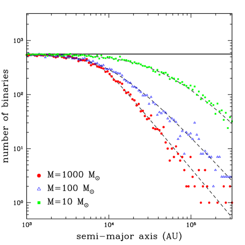
Figure 2.— Binary distributions as a function of semi-major axis. 100,000 binaries are generated following an arbitrarily chosen flat ($\alpha$=1) distribution represented as a thick solid line. The halo density is set to be $\rho_{H}$. The squares, triangles and circles represent binary distributions for three different masses of perturber, after $T=10$ Gyrs evolution. The fitting curves for each model are shown as dashed lines.

4.6. Monte Carlo Algorithm

To test the consistency of the observed binary distribution with the presence of massive perturbers, we must be able to simulate the effect of these perturbers on arbitrary power-law initial distributions. Our basic method for doing this is Monte Carlo simulations in which the initial binary semi-major axis is drawn uniformly from power-law distribution over the interval, $1<\log(a/{\rm AU})<5.5$. The eccentricity is drawn randomly from a distribution uniform in $e^{2}$ (Weinberg, Shapiro & Wasserman, 1987), and the phase and orientation of the orbit are assigned randomly. The perturbers are assumed to have an isotropic Maxwellian velocity distribution relative to the binary center of mass, with a one-dimensional dispersion $\sigma=200{\rm\ km\ s^{-1}}$. This reproduces the true rms velocity, which is a combination of an isothermal-sphere perturber distribution of circular speed $v_{c}=\sqrt{2}\sigma=220{\rm\ km\ s^{-1}}$, and the measured dispersions of halo stars $(\sigma_{\pi},\sigma_{\theta},\sigma_{z})=$ $(170,97,93)~{}{\rm km\ s^{-1}}$ (Popowski & Gould, 1998a, b). In principle, the velocity distribution should be treated as anisotropic. However, this is a higher-order effect, which we ignore in the interest of simplicity.

We consider all impact parameters with $b\lesssim b_{\rm max}={\rm max}\{10b_{\rm min},2a\}$. In particular, we evaluate the $\sim 100$ closest impacts in the tidal regime, even though as we discuss in § 3, the single closest encounter dominates. The mass of each binary component is set to be $0.5{\rm\ M_{\odot}}$. We evolve 100,000 binary systems in each simulation. To illustrate the dependence on the mass of perturbers, we show their effects on an artificial initial binary distribution that is independent of semi-major axis (see Fig. 2). As expected, for the binary systems that are initially tightly bound, the final distributions are almost the same as the initial ones regardless of the mass of the perturbers. However, at wide separations, the distributions are driven to a new power law, which becomes steeper with increasing mass.

This approach works well for any individual initial power-law distribution, but is too time-consuming to process the very large number of distributions required for the comparison of data and models. In § 5.5, we introduce a scattering-matrix formalism that substantially improves the efficiency of mass-production Monte Carlo simulations.

4.7. Fitting Formula

Motivated by the fact that the final distribution is well-approximated by power laws at each extreme, we use a two-line (five-parameter) fitting formula given by,

$$H(x)=\left[f(x)^{-n}+g(x)^{-n}\right]^{-1/n},$$ (10)

where $f(x)$ and $g(x)$ are (two-parameter) straight lines in their argument, $x=\log(a/{\rm AU})$, each corresponding to the respective asymptotic behaviors of $H(x)$. The fifth parameter $n$ permits a smooth transition between $f(x)$ and $g(x)$ in the intermediate region. We calculate the five parameters of equation (10) by minimizing $\chi^{2}$ for a given data set, and the fitting curves for four different masses of perturber are represented as dashed lines in Figure 2.

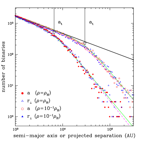
Figure 3.— Evolution of binary distributions with the initial power law, $\alpha=1.567$ obtained in § 2, represented as a thick solid line. 50,000 binaries are evolved in the presence of perturbers of mass 1000${\rm\ M_{\odot}}$ The circles show the binary distributions as functions of semi-major axis while the triangles show the distributions of projected physical separations of the binary components onto the sky plane. The solid lines represent fitting curves for semi-major axis, and the dashed lines for projected physical separation. Two vertical arrows indicate transitions, $a_{t}$, from the unperturbed to the perturbed regimes.

5. Results

Here, we present our main calculations on the evolution of binary distributions with various initial slopes under the influence of various perturber masses and halo densities, and we evaluate the transition separations. Although the semi-major axis of a binary system is a direct indicator of the binding energy of the system and is the theoretically most tractable quantity, it is not observable. It is the angular separations on the sky that we can directly measure from observations. To compare our results with the data, we calculate physical separations projected on the sky plane and convolve these with an adopted distance distribution to predict the binary distributions as a function of angular separation.

In principle, one could compare models directly to the observed projected separations since CG give individual distance estimates to each binary. However, while the observational selection function is quite simple for angular separations (essentially just a pair of $\Theta$-functions), it is rather complex and would be extremely difficult to model for projected physical separations. Hence, we compare our models to the most directly observed quantity: angular separations.

5.1. Semi-Major Axis, $a$

We begin the simulation with a flat distribution, $dN/d\log a\propto const$ for calculation of scattering matrices. We then investigate the dependence of the resulting final binary distribution on perturber mass and halo density. Figure 3 shows a sample of our results with the initial power-law distribution, $dN/d\log a\propto a^{-0.567}$, in agreement with the observations as summarized in § 2. Two models with the same perturber mass but widely different halo densities, $\rho_{H}$ and $10^{-1}\rho_{H}$ are shown. The distributions of semi-major axis are represented by circles.

5.2. Projected Physical Separation, $r_{\perp}$

At $T=10$ Gyr, we calculate the projected physical separation, $r_{\perp}$ of each binary taking account of the randomly chosen orientation to the line of sight and the orbital phase. The distributions of $r_{\perp}$ are shown by triangles in Figure 3.

The two sets of distributions are very similar to each other as demonstrated by the solid and the dashed lines, which are fitted to the points. This can be understood as follows. The time-averaged physical separation is

$$\left<r(e)\right>={1\over 2\pi}\int_{0}^{2\pi}a(1-e~{}{\rm cos}~{}\psi)^{2}{\rm d}\psi=a\left(1+{e^{2}\over 2}\right).$$ (11)

Averaging over the uniform distribution in $e^{2}$ yields $\left<r\right>=5a/4$, and projecting onto the sky plane gives,

$$\left<r_{\perp}\right>={\pi\over 4}\left<r\right>={5\pi\over 16}a\simeq 0.98a.$$ (12)

That is, the triangles are, on average, slightly shifted to left of the circles in Figure 3.

There is, however, a deviation from equation (12) at large projected physical separation. We find that a binary system with a highly eccentric orbit is more likely to be disturbed than one with a circular orbit. Since the highly eccentric systems are selectively destroyed for loosely bound binary systems, the distribution in eccentricity is no longer isotropic, and the actual projected physical separations differ from equation (12). We therefore use numerical calculations of the projected physical separations rather than the analytic estimate of equation (12).

5.3. Transition Separation, $a_{t}$

Using the five-parameter fitting formula from equation (10), we calculate the asymptotic slopes for distributions in semi-major axis. These are represented as solid curves in Figure 3. The intersection of these asymptotic slopes characterizes the transition $a_{t}$ from the unperturbed to the perturbed regime. The two arrows in Figure 3 represent the intersections for two different halo densities. As predicted by equation (3), the transition for a denser halo model occurs at smaller separation, $a_{t}\propto\rho^{-2/3}$.

The transition separations for various perturber mass and halo densities are shown in Figure 4, which provides a qualitative understanding of the underlying physics of binary disruption and is in a good accord with the prediction of equation (3) and (6). In particular, in the tidal regime the transition separation is independent of perturber mass, and is a function of halo density $a_{t}\propto\rho^{-2/3}$, although the actual values of $a_{t}$ are a factor of $2$ smaller than those predicted by equation (3). At smaller mass, the transition separation grows roughly as $a_{t}\propto M^{-1}$, as predicted by equation (6) for the Coulomb regime.

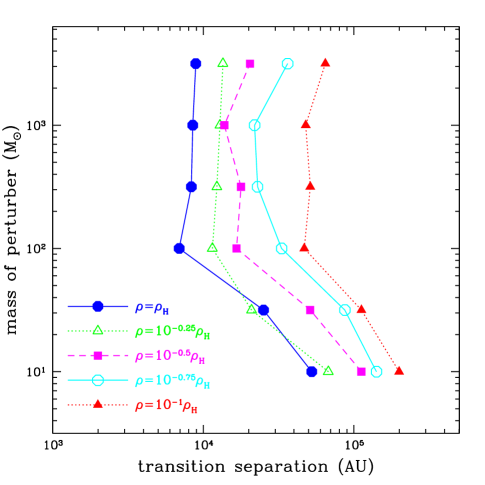
Figure 4.— Transition separations $a_{t}$ for different halo densities as a function of perturber mass. Transition separations are obtained for each model by calculating the intersection of $f(x)$ and $g(x)$ in eq. (10).

5.4. Angular Separation, $\Delta\theta$

To predict the observed angular distribution function, we must convolve the model’s projected-separation distribution function with an assumed distribution of (inverse) distances to the binaries in the sample.

We derive this distribution from the observed distances of the 90 binaries in the CG sample. To understand our procedure for doing so, consider first the idealized case of binaries drawn from a distance-limited sample of uniform density. Of course, in this case, the distance distribution would be $dN/d\log R\propto R^{3}\Theta(R_{\rm max}-R)$, where $\Theta$ is a step function, and $R_{\rm max}$ is the distance limit. However, the binaries selected at fixed $\Delta\theta$ would not be distributed as $R^{3}$. This is because the binaries at distances $R_{1}$ and $R_{2}$ would have projected separations $r_{\perp,1}=R_{1}\Delta\theta$ and $r_{\perp,2}=R_{2}\Delta\theta$, and these differ in frequency (for fixed log intervals) in the ratio $(r_{\perp,1}/r_{\perp,2})^{1-\alpha}$, where $\alpha=1.567$ is the binary-separation power-law slope. Hence, the sample distribution would be $dN_{\rm sample}/d\log R\propto R^{4-\alpha}\Theta(R_{\rm max}-R)$. Therefore, to obtain an estimate of the underlying distribution of distances that yields the observed sample distribution, we simply adopt the observed distribution, but weight each binary by $R^{\alpha-1}$. We estimate $R$ for each binary by applying the fourth-order color-magnitude relation of CG to the brighter component, except when that component has no $J$-band data, in which case we use the fainter component.

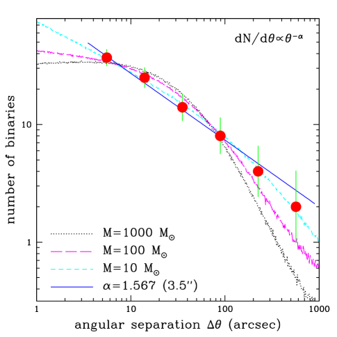
Figure 5.— The best-fit final binary distributions for various perturber masses, assuming that the initial distribution is a power-law. The halo density is set to be $\rho_{\rm H}$. The observed halo binary distribution (Fig. 1) is shown for comparison. A model with 1000 $M_{\odot}$ perturber deviates significantly from the observations while a model with 10 $M_{\odot}$ is quite consistent with them.

5.5. Scattering Matrix, $\bf{S}$

To simultaneously investigate large subsets of initial power-law distributions for each model specified by $M$ and $\rho$, we use a Monte Carlo simulation (see § 4.6) with an initially flat ($dN/d\log a\propto const$) distribution to construct a scattering matrix, ${\bf{S}}_{ij}(M,\rho)$, the relative probability that a binary with initial log semi-major axis, $\log a_{j}$ will finally be observed in the angular separation bin, $\log\Delta\theta_{i}$. Explicitly,

$${\bf{S}}_{ij}(M,\rho)=\sum_{k}\int{\rm d}\log R{dN\over d\log R}\delta\left[\log R\Delta\theta_{i}-\log r_{\perp,j}(k;M,\rho)\right],$$ (13)

where $r_{\perp,j}(k;M,\rho)$ is the final projected separation of a binary with initial semi-major axis $a_{j}$ in $k^{th}$ realization of a Monte Carlo simulation of perturbers with mass $M$ and density $\rho$. In practice, since the radial profile $dN/d\log R$ is estimated directly from the binary data as discussed in § 5.4, we evaluate equation (13) by discretely summing over the $l=1\ldots 90$ binaries,

$${\bf{S}}_{ij} (M,\rho) =\sum_{k}\sum_{l=1}^{90}R_{l}^{\alpha-1}$$

$$\times\Theta\left({\delta\log\Delta\theta\over 2}-|\log R_{l}\Delta\theta_{i}-\log r_{\perp,j}(k;M,\rho)|\right),$$

where $\delta\log\Delta\theta$ is the logarithmic width of the $\Delta\theta$ bins.

Since the simulations are calculated from a flat distribution, i.e., equal number of binaries per logarithmic semi-major axis bin, the un-normalized probability of finding binaries at $\Delta\theta$ for a given dark-matter model is then given by,

$$P(\Delta\theta_{i};M,\rho,\alpha)={\bf{S}}_{ij}(M,\rho)w(a_{j};\alpha),$$ (15)

where $w(a_{j};\alpha)=a_{j}^{1-\alpha}$ is the power-law of the initial binary distribution, $dN/da\propto a^{-\alpha}$.

6. Dark Matter Limits

For each model, we fix the normalization so that the number expected in the interval $3.\!\!\arcsec 5<\Delta\theta<900\arcsec$ is equal to 90, i.e., the total number observed over this interval. We call the normalized resulting function $P_{\rm N}(\Delta\theta;M,\rho,\alpha)$, evaluate the likelihood of a given model as a sum over the 90 observed binaries,

$$\ln L(M,\rho,\alpha)=\sum_{i=1}^{90}\ln P_{\rm N}(\Delta\theta_{i};M,\rho,\alpha),$$ (16)

and find the maximum likelihood over various initial slopes $\alpha$,

$$\ln L(M,\rho)\equiv\max_{\alpha}\left\{\ln L(M,\rho,\alpha)\right\}.$$ (17)

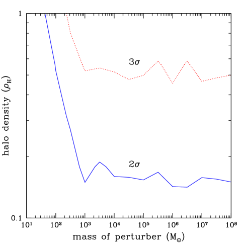
Figure 6.— Exclusion contour plot for halo dark-matter models. Various confidence levels are shown. The oscillations at high masses are due to numerical noise.

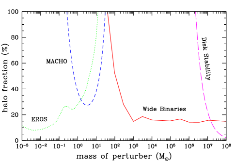
Figure 7.— Exclusion contour plot at 95% confidence level. The dashed, the dotted and the long dashed lines represent the microlensing-based limits from EROS (Afonso et al., 2003) and MACHO (Alcock et al., 2001), and the limit based on disk stability (Lacey & Ostriker, 1985), respectively. Our limits from the $3.\!\!\arcsec 5<\Delta\theta<900\arcsec$ sample are represented as a solid line.

Figure 5 shows the normalized resulting functions for various perturber masses with $\rho=\rho_{\rm H}$. For 1000 $M_{\odot}$ perturbers, the likelihood is maximized by an initial distribution that is nearly flat. However, no initial power-law is consistent with the observed distribution. For low mass perturbers, by contrast, the likelihood is maximized by an initial slope that is only slightly shallower than the observed one, and the resulting distribution is consistent with observations.

We compare the resulting likelihoods to $L(0,0)$, i.e., the model with no dark-matter perturbers, which is characterized by the best fit slope $\alpha=1.567$, and we define confidence levels by

$$\sigma(M,\rho)=\sqrt{2\left[\ln L(0,0)-\ln L(M,\rho)\right]}.$$ (18)

As we discussed in § 2, the fact that the binary sample is clearly incomplete for $\Delta\theta<3.\!\!\arcsec 5$ implies that it may also be slightly incomplete for binaries just above this threshold. However, one can see from the form of the normalized resulting functions in Figure 5 that such incompleteness would actually favor models with massive perturbers over the no-perturber model. We verify numerically that this indeed is the sign of the bias. Hence our choice of the $\Delta\theta\geq 3.\!\!\arcsec 5$ threshold is conservative in the face of possible incompleteness.

Figure 6 shows the resulting contour plot excluding various dark-matter models at various confidence ($\sigma$) levels. Finally, in Figure 7 we compare our 95% confidence ($2\sigma$) limits with those from the EROS (Afonso et al., 2003) and MACHO (Alcock et al., 2001) microlensing collaborations. The halo binaries exclude models that have generally higher MACHO masses than those probed by these microlensing experiments. Moreover, they extend all the way to the Lacey & Ostriker (1985) limit based on stability of the Galactic disk.

All three curves in Figure 7 show limits on models with $\delta$-function mass distributions. However any model with broader distribution of mass but total density $\rho_{H}$, would be ruled out provided that the combined limits from the three curves ruled out each mass separately.

Hence, the only remaining window open for MACHOs would be black holes with a mass function strongly peaked at $M\sim 35~{}{\rm\ M_{\odot}}$. Even this model is more strongly constrained than shown Figure 7 because the MACHO (Alcock et al., 2001) results and our results each separately place weak limits on this model, which when combined comes close to ruling it out.

7. Conclusions

In this paper, we have investigated the evolution of halo wide binaries in the presence of MACHOs and estimated upper limits of MACHO density as a function of their assumed mass by comparing our simulations to the sample of halo wide binaries of CG. We exclude MACHOs with masses $M>43{\rm\ M_{\odot}}$ at the standard local halo density $\rho_{H}$ at the 95% confidence level.

MACHOs have been a major dark-matter candidate ever since observations first established that this mysterious substance dominates the mass of galaxies. Prodigious efforts over several decades have gradually whittled down the mass range allowed to this dark-matter candidate. However, the window for MACHOs with $30{\rm\ M_{\odot}}\lesssim M\lesssim 10^{3}{\rm\ M_{\odot}}$ remained completely open while constraints in the range $10^{3}{\rm\ M_{\odot}}\lesssim M\lesssim 10^{6}{\rm\ M_{\odot}}$ were somewhat model dependent. Our new limits on MACHOs $M>43{\rm\ M_{\odot}}$ all but close this window.

Appendix A Ionized Binaries

After disruption of a binary system, the two ionized members remain in similar Galactic orbit, so it is only the separation along the direction of the orbital motion that can keep increasing, while the perpendicular separation oscillates.

In the Coulomb regime, the average post-ionization gain in the relative velocity of binaries along the orbital direction is (see eq.[5]),

$$\sqrt{\left<v^{2}_{\parallel}\right>}=\sqrt{{32\pi G^{2}\rho M\Delta t\over 3v}\ln\Lambda},$$ (A1)

where $\Delta t$ is the remaining time to 10 Gyr after disruption. For a diffusive process that is uniform over time $\Delta t$, the root-mean-square separation parallel to the orbital motion is

$$\sqrt{\left<d_{\parallel}^{2}\right>}=\sqrt{\left<v^{2}_{\parallel}\right>{\Delta t^{2}\over 3}}=2000~{}{\rm pc}\left({\rho\over\rho_{H}}\right)^{1/2}\left(M\over 30M_{\odot}\right)^{1/2}\left({v\over 300~{}{\rm km\ s^{-1}}}\right)^{-1/2}\left({\ln\Lambda\over 5.1}\right)^{1/2}\left({\Delta t\over 10~{}{\rm Gyr}}\right)^{3/2},$$ (A2)

where the Coulomb logarithm is calculated at the scaled quantities.

For a conservative limit of the tidal radius, $a_{t}=3$ pc, the time required for ionized binaries to separate farther than $a_{t}$ is 0.13 Gyr, so that only binaries ionizing within the last $\sim$ 1% of the age of the Galaxy have a significant chance to be confused with bound systems, even for the lowest mass perturbers that we can effectively probe. In the tidal limit, binaries escape with characteristic velocities of the transition separation $\sim 10^{4}$ AU, i.e., 300 $\rm m\ s^{-1}$. Hence, they drift one tidal radius in only 10 Myr, so their impact is even smaller. Nevertheless, since there are only a handful of binaries in the widest-separation bins, it is important to make a careful estimate of the contribution from ionizing binaries. We take account of ionized binaries in the simulations as follows. Binaries are considered ionized either when they have positive energy or they have $a>a_{t}$. They are then assigned a relative velocity equal to their escape velocity in the former case, or zero in the latter. A random orbital direction is chosen. The ionized binaries in the Coulomb regime then continue to suffer perturbations to the end of the simulations whose effect we calculate using equation (A1) and (A2). At the end of the simulation, the binary is assigned a transverse separation drawn randomly from a sinusoidal distribution of amplitude,

$$d_{\perp,{\rm MAX}}={v_{\perp}\over\Omega}=26~{}{\rm pc}~{}\left({v_{\perp}\over{\rm km\ s^{-1}}}\right),$$ (A3)

where $v_{\perp}$ is the final transverse velocity, $\Omega=\sqrt{2}v_{c}/R_{0}$ is the epicyclic frequency, and $R_{0}$ is the Galactocentric distance. Finally, we “observe” the ionized binary from a random orientation and record the projected separation. We find that the ionized binaries have no significant effect either on the final distribution or the calculated likelihoods. We ignore ionized binaries in the tidal regime because these escape with much higher initial velocities and because these velocities grow much more rapidly than indicated by equation (A1).

References

- Afonso et al. (2003) Afonso, C., et al. 2003, A&A, 400, 951
- Alcock et al. (1998) Alcock. C., et al. 1998, ApJ, 499, L9
- Alcock et al. (2001) Alcock. C., et al. 2001, ApJ, 550, L169