Magnetohydrodynamic Jump Conditions for Oblique Relativistic Shocks
with Gyrotropic Pressure

Abstract

Shock jump conditions, i.e., the specification of the downstream parameters of the gas in terms of the upstream parameters, are obtained for steady-state, plane shocks with oblique magnetic fields and arbitrary flow speeds. This is done by combining the continuity of particle number flux and the electromagnetic boundary conditions at the shock with the magnetohydrodynamic conservation laws derived from the stress-energy tensor. For ultrarelativistic and nonrelativistic shocks, the jump conditions may be solved analytically. For mildly relativistic shocks, analytic solutions are obtained for isotropic pressure using an approximation for the adiabatic index that is valid in high sonic Mach number cases. Examples assuming isotropic pressure illustrate how the shock compression ratio depends on the shock speed and obliquity. In the more general case of gyrotropic pressure, the jump conditions cannot be solved analytically without additional assumptions, and the effects of gyrotropic pressure are investigated by parameterizing the distribution of pressure parallel and perpendicular to the magnetic field. Our numerical solutions reveal that relatively small departures from isotropy (e.g., $\sim 20$%) produce significant changes in the shock compression ratio, $r$, at all shock Lorentz factors, including ultrarelativistic ones, where an analytic solution with gyrotropic pressure is obtained. In particular, either dynamically important fields or significant pressure anisotropies can incur marked departures from the canonical gas dynamic value of $r=3$ for a shocked ultrarelativistic flow and this may impact models of particle acceleration in gamma-ray bursts and other environments where relativistic shocks are inferred. The jump conditions presented apply directly to test-particle acceleration, and will facilitate future self-consistent numerical modeling of particle acceleration at oblique, relativistic shocks; such models include the modification of the fluid velocity profile due to the contribution of energetic particles to the momentum and energy fluxes.

1 INTRODUCTION

Collisionless shocks are pervasive throughout space and are regularly associated with objects as diverse as stellar winds, supernova remnants, galactic and extra-galactic radio jets, and accretion onto compact objects. Relativistic shocks, where the shock speed is close to the speed of light, may be generated by the most energetic events; for example, pulsar winds, blastwaves in quasars and active galactic nuclei (e.g., Blandford & McKee, 1977), and in gamma-ray bursts (e.g., Piran, 1999). They may naturally emerge as the evolved products of Poynting flux-driven or matter-dominated outflows in the vicinity of compact objects such as neutron stars and black holes. As relativistic shocks propagate through space, magnetic fields upstream from the shock, at even small angles with respect to the shock normal, are strongly modified by the Lorentz transformation to the downstream frame. The downstream magnetic fields are both increased and tilted toward the plane of the shock and can have large angles with respect to the shock normal. Hence, most relativistic shocks can be expected to see highly oblique magnetic fields and oblique magnetohydrodynamic (MHD) jump conditions are required to describe them.

Relativistic shock jump conditions have been presented in a variety of ways over the years. The standard technique for deriving the equations is to set the divergence of the stress-energy tensor equal to zero on a thin volume enclosing the shock plane and use Gauss’s theorem to generate the jump conditions across the shock. For example, Taub (1948) developed the relativistic form of the Rankine-Hugoniot relations, using the stress-energy tensor with velocity expressed in terms of the Maxwell-Boltzmann distribution function for a simple gas. de Hoffmann & Teller (1950) presented a relativistic MHD treatment of shocks in various orientations and a treatment of oblique shocks for the nonrelativistic case, eliminating the electric field by transforming to a frame where the flow velocity is parallel to the magnetic field vector (now called the de Hoffmann-Teller frame). Peacock (1981), following Landau & Lifshitz (1959), presented jump conditions without electromagnetic fields, and Blandford & McKee (1976), also using the approach of Landau & Lifshitz (1959) and Taub (1948), developed a concise set of jump conditions for a simple gas using scalar pressure. Webb, Zank, & McKenzie (1987) provided a review of relativistic MHD shocks in ideal, perfectly conducting plasmas, and in particular the treatment by Lichnerowicz (1967, 1970), which used this approach to develop the relativistic analog of Cabannes’ shock polar (Cabannes, 1970), whose origins also lie in Landau & Lifshitz (1959). Kirk & Webb (1988) developed hydrodynamic equations using a pressure tensor, and Appl & Camenzind (1988) developed relativistic shock equations for MHD jets using scalar pressure and magnetic fields with components $B_{z}$ and $B_{\phi}$ (a parallel field with a twist). Ballard & Heavens (1991) derived MHD jump conditions using the stress-energy tensor with isotropic pressure and the Maxwell field tensor. By using a Lorentz transformation to the de Hoffman-Teller frame, they restricted shock speeds, $u_{0}$, to $u_{0}/c<\cos{\Theta_{\mathrm{B}}}$, where $\Theta_{\mathrm{B}}$ is the angle between the shock normal and the upstream magnetic field and $c$ is the speed of light; hence, this approach may only be used for mildly relativistic applications.

All of these approaches assumed that particles encountered by the shock did not affect the shock structure, i.e., shocked particles were treated as test particles. Moreover, except for Kirk & Webb (1988), they confined their analyses to cases of isotropic pressures, a restriction that is appropriate to thermal particles or very energetic ones subject to the diffusion approximation in the vicinity of non-relativistic shocks. The assumption of pressure isotropy must be relaxed when considering the hydrodynamics of relativistic shocks, since their inherent nature imposes anisotropy on the ion and electron distributions: this is due to the difficulty particles have streaming against relativistic flows. The computed particle anisotropies for relativistic shocks are considerable in the shock layer (e.g., Bednarz & Ostrowski, 1998; Kirk et al., 2000), persisting up to arbitrarily high ultrarelativistic energies. The particles eventually relax to isotropy in the fluid frame far downstream, on length scales comparable to diffusive ones. However, only a small minority of accelerated particles achieve isotropy in the upstream fluid frame of relativistic shocks, due to the rapid convection to the downstream side of the flow discontinuity. These isotropized particles are present only when they manage to diffuse more than a diffusive mean free path, $\lambda$, upstream of the shock; their contribution to the flow dynamics is therefore dominated by that of the anisotropic particles within a distance $\lambda$ of the shock. For non-linear particle acceleration, where the non-thermal ion or electron populations possess a sizable fraction of the total energy or momentum fluxes, calculating pressure anisotropy will be critical for determining the conservation of these fluxes through the shock transition (e.g., Ellison, Baring, & Jones, 1996). The jump conditions we develop here can serve as a guide to self-consistent solutions of non-linear relativistic shock acceleration problems (Ellison & Double, 2002).

Here, we extend previous work by deriving a set of fully relativistic MHD jump conditions with gyrotropic pressure and oblique magnetic fields. We adopt the gyrotropic case as a specialized generalization because it (i) is exactly realized in plane-parallel shocks and is a good approximation for oblique shocks where the flow deflection is small, i.e., the field plays a passive role (generally high Alfvénic Mach number cases), and (ii) permits a comparatively simple expression of the Rankine-Hugoniot jump conditions. The sonic Mach number, $M_{\mathrm{S}}$, used throughout our paper, refers to the shock speed compared to the fast-mode magnetosonic wave speed as described in Kirk & Duffy (1999), i.e., $M_{\mathrm{S}}\equiv\sqrt{3\rho_{0}u_{0}^{2}/(5P_{0})}$, where $\rho_{0}$ is the upstream mass density and $P_{0}$ is the upstream pressure. The Alfvén Mach number we refer to here is defined as $M_{\mathrm{A}}\equiv\sqrt{4\pi\rho_{0}u_{0}^{2}}/B_{0}$ ($B_{0}$ is the upstream magnetic field), regardless of the shock Lorentz factor, $\gamma_{0}=[1-(u_{0}/c)^{2}]^{-1/2}$; i.e., we use these definitions applicable to non-relativistic flows as parameters for the depiction of our results at all $\gamma_{0}$.

Our results are not restricted to the de Hoffmann-Teller frame and apply for arbitrary shock speeds and arbitrary shock obliquities. We solve these equations and determine the downstream state of the gas in terms of the upstream state first for the special case of isotropic pressure, and then, by parameterizing the ratio of pressures parallel and perpendicular to the magnetic field, for cases of gyrotropic pressure.

A principal result of this analysis is that either dynamically important magnetic fields or significant pressure anisotropies produce marked departures from the canonical value (e.g., Blandford & McKee, 1976; Kirk & Duffy, 1999) of $r=3$ for the shock compression ratio in an ultrarelativistic fluid. The magnetic weakening of ultrarelativistic perpendicular shocks came to prominence in the work of Kennel & Coroniti (1984) on the interaction of the Crab pulsar’s wind with its environment. The similarity of such consequences of fluid anisotropy and low Alfvénic Mach number fields, which are also pervasive for trans-relativistic and non-relativistic shocks, has its origin in the similar nature of the plasma and electromagnetic contributions to the spatial components of the stress-energy tensor. This result may have important implications for the application of first-order Fermi shock acceleration theory to gamma-ray bursts and jets in active galaxies.

In this work, we concentrate on using analytic methods for determining the fluid and electromagnetic characteristics of the shock and do not explicitly include first-order Fermi particle acceleration. Future work will combine these results with Monte Carlo techniques (e.g., Ellison, Baring, & Jones, 1996; Ellison & Double, 2002) that will allow the modeling of Fermi acceleration of particles, including the modification of the shock structure resulting from the backreaction of energetic particles on the upstream flow at all pertinent length scales. The jump conditions we present here, however, apply directly to test-particle Fermi acceleration in shocks with arbitrary speed and obliquity.

2 DERIVATION OF MHD JUMP CONDITIONS

2.1 Steady-State, Planar Shock

Using a Cartesian coordinate system with the $+x$-axis pointing towards the downstream direction, we consider an infinite, steady-state, plane shock traveling to the left at a speed $u_{0}$ with its velocity vector parallel to the normal of the plane of the shock as shown in Figure 1. The upstream fluid consists of a thin, nonrelativistic plasma of protons and electrons in thermal equilibrium with $\mathcal{T}_{p0}=\mathcal{T}_{e0}$, where $\mathcal{T}_{p0}$ ($\mathcal{T}_{e0}$) is the unshocked proton (electron) temperature. A uniform magnetic field, $B_{0}$, makes an angle $\Theta_{\mathrm{B0}}$ with respect to the $x$-axis as seen from the upstream plasma frame. We keep the field weak enough to insure high Alfvén Mach numbers (i.e., $M_{\mathrm{A}}\gtrsim 2.5$) and thus to insure that the magnetic turbulence responsible for scattering the particles is frozen into the plasma. The $xyz$ coordinate system is oriented such that there are only two components of magnetic field, $B_{x0}$ and $B_{z0}$, in the upstream frame. The field will remain co-planar in the downstream frame and the downstream flow speed will be confined to the $x$-$z$ plane as well (e.g., Jones & Ellison, 1987).

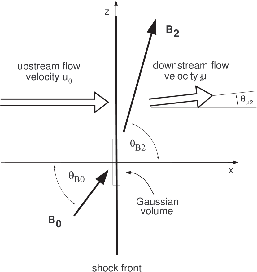
Figure 1: Schematic diagram of a plane shock, viewed from the shock frame, showing oblique magnetic fields and a Gaussian volume over which the divergence of the stress-energy tensor is integrated. The angles and field strengths are measured in the local plasma frame and, in all of our examples, we take the upstream flow to be parallel to the shock normal. The $y$-axis is directed into the page.

In the shock frame, the upstream flow is in the $+x$-direction and is described by the normalized four-velocity: $\beta^{\nu}_{0}=\gamma_{0}(1,\beta_{0}^{x},0,0)$. The downstream (i.e., shocked) flow four-velocity is $\beta^{\nu}_{2}=\gamma_{2}(1,\beta_{2}^{x},0,\beta_{2}^{z})$, where the subscript 0 (2) refers, here and elsewhere, to upstream (downstream) quantities, $\beta$ $=\mathbf{u}/c$, and $\gamma=(1-\beta^{2})^{-1/2}$ is the corresponding Lorentz factor associated with the magnitude of the flow three-velocity $\mathbf{u}$. Note that these subscript conventions follow those used in Ellison, Berezhko, & Baring (2000), where the subscript 1 is reserved for positions infinitesimally upstream of the subshock discontinuity, admitting the possibility of flow and field gradients upstream of the subshock. Here the use of subscript 1 is redundant. In addition, greek upper and lower indices refer to spacetime components 0–3, while roman indices refer to space components 1–3.

The set of equations connecting the upstream and downstream regions of a shock consist of the continuity of particle number flux (for conserved particles), momentum and energy flux conservation, plus electromagnetic boundary conditions at the shock interface, and the equation of state. The various parameters that define the state of the plasma, such as pressure and magnetic field, are determined in the plasma frame and must be Lorentz transformed to the shock frame where the jump conditions apply. We assume that the electric field is zero in the local plasma rest frame. In general, the six jump conditions plus the equation of state cannot be solved analytically because the adiabatic index (i.e., the ratio of specific heats, whose value varies smoothly between the nonrelativistic and ultrarelativistic limits) is a function of the downstream plasma parameters, creating an inherently nonlinear problem (e.g., Ellison & Reynolds, 1991). Even with the assumption of gyrotropic pressure, there are more unknowns than there are equations; however, with additional assumptions, approximate analytic solutions may be obtained.

2.2 Transformation Properties of the Stress-Energy Tensor

The stress-energy tensor, $T^{\mu\nu}$, describes the matter and electromagnetic momentum and energy content of a medium at any given point in space-time. Continuity across the shock is established by setting the appropriate divergence (or covariant derivative $T^{\mu\nu}_{\ \ \ ;\nu}$) of the stress-energy tensor equal to zero, namely for directions locally normal to the shock. Following standard expositions such as Tolman (1934) and Weinberg (1972), the total stress-energy tensor, $T^{\mu\nu}_{\mathrm{tot}}$, is expressed as the sum of fluid and electromagnetic parts, i.e.,

$$T^{\mu\nu}_{\mathrm{tot}}=T^{\mu\nu}_{\mathrm{fluid}}+T^{\mu\nu}_{\mathrm{EM}}\ .$$ (1)

This is then integrated over a thin volume containing the shock plane as shown in Figure 1. Application of Gauss’s theorem then yields the energy and momentum flux conditions across the plane of the shock by using $T^{\mu\nu}n_{\nu}=0$. Accordingly, $T^{0\nu}n_{\nu}$ yields the conservation of energy flux, $T^{1\nu}n_{\nu}$ yields the $x$-contribution to momentum flux conservation in the $x$-direction, $T^{3\nu}n_{\nu}$ yields the $z$-contribution to momentum flux conservation in the $x$-direction, and $n_{\nu}=(0,1,0,0)$ is the unit four-vector along the $x$-axis in the reference frame of the shock. The Einstein summation convention is adopted here and elsewhere in this paper.

The components of the fluid and electromagnetic tensors are defined in the local plasma frame and are subsequently Lorentz-transformed to the shock frame where the flux conservation conditions apply, i.e.,

$$T^{\mu\nu}_{\mathrm{tot,s}}=\Lambda^{\mu}_{\alpha}\left[T_{\mathrm{fluid,n}}^{\alpha\beta}+T_{\mathrm{EM,n}}^{\alpha\beta}\right]\Lambda^{\nu}_{\beta}\ ,$$ (2)

where the subscript $n$ ($s$) refers to the plasma (shock) frame with the $x$-axis oriented normal to the shock in each case. Since the flow speeds in our model may have two space components, in the $x$- and $z$-directions, the Lorentz transformation is

$$\Lambda^{\mu}_{\alpha}=\left(\begin{array}[]{cccc}\gamma&\gamma\beta_{x}&0&\gamma\beta_{z}\\[8.5359pt] \gamma\beta_{x}&1+\hbox{${{\displaystyle\gamma-1\vphantom{(}}\over{\displaystyle\beta^{2}\vphantom{(}}}$}\beta_{x}^{2}&0&\hbox{${{\displaystyle\gamma-1\vphantom{(}}\over{\displaystyle\beta^{2}\vphantom{(}}}$}\beta_{x}\beta_{z}\\[11.38092pt] 0&0&1&0\\[11.38092pt] \gamma\beta_{z}&\hbox{${{\displaystyle\gamma-1\vphantom{(}}\over{\displaystyle\beta^{2}\vphantom{(}}}$}\beta_{z}\beta_{x}&0&1+\hbox{${{\displaystyle\gamma-1\vphantom{(}}\over{\displaystyle\beta^{2}\vphantom{(}}}$}\beta_{z}^{2}\end{array}\right)\ ,$$ (3)

where the $\beta$ components and $\gamma$ are as previously defined in Section 2.1. The system defined in Figure 1 is invariant under translations in the $y$-direction, so that conservation laws along the $y$-axis are trivially satisfied.

2.3 The Fluid Tensor and Equation of State

The fluid tensor will be constrained to the gyrotropic case in the local fluid frame; i.e., pressure can have one value parallel to the magnetic field and a different value perpendicular to the magnetic field (with symmetry about the magnetic field vector). This gives the diagonal stress-energy tensor

$$T_{\mathrm{fluid,B}}=\left(\begin{array}[]{cccc}e&0&0&0\\ 0&P_{\|}&0&0\\ 0&0&P_{\perp}&0\\ 0&0&0&P_{\perp}\end{array}\right)\ ,$$ (4)

where $e$ is the total energy density, $P_{\|}$ ($P_{\perp}$) is the pressure parallel (perpendicular) to the magnetic field, and the subscript $B$ refers to the magnetic axis in the plasma frame. We obtain the fluid tensor in the $xyz$ plasma frame (labelled with subscript $n$ referring to the shock normal), $T_{\mathrm{fluid,n}}$, with a rotation about the $y$-axis,

$$T_{\mathrm{fluid,n}}\;=\;\mathcal{R}\;T_{\mathrm{fluid,B}}\;\mathcal{R}^{-1}\ ,$$ (5)

where

$$\mathcal{R}=\left(\begin{array}[]{cccc}1&0&0&0\\ 0&\cos\Theta_{\mathrm{B}}&0&\sin\Theta_{\mathrm{B}}\\ 0&0&1&0\\ 0&-\sin\Theta_{\mathrm{B}}&0&\cos\Theta_{\mathrm{B}}\end{array}\right)\ .$$ (6)

The resulting tensor in the xyz plasma frame is

$$T_{\mathrm{fluid,n}}=\left(\begin{array}[]{cccc}e&0&0&0\\ 0&P_{\|}\cos^{2}{\Theta_{\mathrm{B}}}+P_{\perp}\sin^{2}{\Theta_{\mathrm{B}}}&0&(P_{\perp}-P_{\|})\sin{\Theta_{\mathrm{B}}}\cos{\Theta_{\mathrm{B}}}\\ 0&0&P_{\perp}&0\\ 0&(P_{\perp}-P_{\|})\sin{\Theta_{\mathrm{B}}}\cos{\Theta_{\mathrm{B}}}&0&P_{\perp}\cos^{2}{\Theta_{\mathrm{B}}}+P_{\|}\sin^{2}{\Theta_{\mathrm{B}}}\end{array}\right)\ ,$$ (7)

with the $T^{ij}$ space components corresponding to the 3-dimensional pressure tensor presented by Ellison, Baring, & Jones (1996) for nonrelativistic shocks, once a typographical error is corrected.

Renaming the components of the fluid tensor as

$$T_{\mathrm{fluid,n}}=\left(\begin{array}[]{cccc}e&0&0&0\\[2.84544pt] 0&P_{xx}&0&P_{xz}\\[5.69046pt] 0&0&P_{yy}&0\\[5.69046pt] 0&P_{zx}&0&P_{zz}\end{array}\right)\ ,$$ (8)

with $P_{xz}=P_{zx}$, we have the identities

$$P_{\|}=P_{xx}-P_{xz}\hbox{${{\displaystyle\sin{\Theta_{\mathrm{B}}}\vphantom{(}}\over{\displaystyle\cos{\Theta_{\mathrm{B}}}\vphantom{(}}}$}\ ,$$ (9)

$$P_{\perp}=P_{xx}+P_{xz}\hbox{${{\displaystyle\cos{\Theta_{\mathrm{B}}}\vphantom{(}}\over{\displaystyle\sin{\Theta_{\mathrm{B}}}\vphantom{(}}}$}\ ,$$ (10)

and,

$$P_{zz}=P_{xx}+2P_{xz}\cot{(2\Theta_{\mathrm{B}})}\ .$$ (11)

The $T^{00}$ component, $e$, is the total energy density in the rest or plasma frame. The other components, $P_{ij}$, are defined by Tolman (1934) as the “absolute stress” components in the proper frame. $P_{ij}$ is the pressure parallel to the $i$-axis exerted on a unit area normal to the $j$-axis. Hence, the diagonal components can be considered a pressure, but the off-diagonal components are shear stresses. The isotropic scalar pressure, $P=Tr(\mathcal{P}_{\mathrm{fluid,B}})/3$, is a Lorentz invariant. The fluid tensor, in general, changes its appearance significantly under a Lorentz transformation via the mixing of components: for example, it picks up momentum flux components in reference frames moving with respect to the proper frame (Tolman, 1934).

Using the above expressions, we can derive an adiabatic equation of state. Starting with the spatial portion of the fluid tensor:

$$\mathcal{P}_{\mathrm{fluid,B}}=\left(\begin{array}[]{ccc}P_{\|}&0&0\\ 0&P_{\perp}&0\\ 0&0&P_{\perp}\end{array}\right)\ ,$$ (12)

the total energy density can be written as

$$e=\hbox{${{\displaystyle Tr(\mathcal{P}_{\mathrm{fluid,B}})\vphantom{(}}\over{\displaystyle 3(\Gamma-1)\vphantom{(}}}$}+\rho c^{2}\ ,$$ (13)

where $Tr(\mathcal{P}_{\mathrm{fluid,B}})$ is the trace of the pressure tensor, $\Gamma$ is the adiabatic index, and $\rho c^{2}$ is the rest mass energy density. Using equations (9) and (10),

$$\hbox{${{\displaystyle Tr(\mathcal{P}_{\mathrm{fluid,B}})\vphantom{(}}\over{\displaystyle 3(\Gamma-1)\vphantom{(}}}$}=\hbox{${{\displaystyle 1\vphantom{(}}\over{\displaystyle 3(\Gamma-1)\vphantom{(}}}$}(P_{\parallel}+2P_{\perp})=\hbox{${{\displaystyle 1\vphantom{(}}\over{\displaystyle\Gamma-1\vphantom{(}}}$}\left[P_{xx}+\hbox{${{\displaystyle P_{xz}\vphantom{(}}\over{\displaystyle 3\vphantom{(}}}$}\left(2\cot{\Theta_{\mathrm{B}}}-\tan{\Theta_{\mathrm{B}}}\right)\right]\ .$$ (14)

In terms of the magnetic field, where $\tan\Theta_{\mathrm{B}}=B_{z}/B_{x}$, the adiabatic, gyrotropic equation of state becomes

$$e=\hbox{${{\displaystyle 1\vphantom{(}}\over{\displaystyle\Gamma-1\vphantom{(}}}$}\left[P_{xx}+\hbox{${{\displaystyle P_{xz}\vphantom{(}}\over{\displaystyle 3\vphantom{(}}}$}\left(2\hbox{${{\displaystyle B_{x}\vphantom{(}}\over{\displaystyle B_{z}\vphantom{(}}}$}-\hbox{${{\displaystyle B_{z}\vphantom{(}}\over{\displaystyle B_{x}\vphantom{(}}}$}\right)\right]+\rho c^{2}\ .$$ (15)

While $\Gamma$ is well defined in the nonrelativistic and fully relativistic limits, in mildly relativistic shocks $\Gamma$ depends on an unknown relation between $e$ and $P$ which we will address in a later section.

2.4 The Electromagnetic Tensor

The electric and magnetic field components of the general electromagnetic tensor in the plasma frame are given by Tolman (1934) as

$$T_{\mathrm{EM,n}}\;=\;\hbox{${{\displaystyle 1\vphantom{(}}\over{\displaystyle 4\pi\vphantom{(}}}$}\left(\begin{array}[]{cccc}\hbox{${{\displaystyle E^{2}+B^{2}\vphantom{(}}\over{\displaystyle 2\vphantom{(}}}$}&\left(\mathbf{E}\times\mathbf{B}\right)_{x}&\left(\mathbf{E}\times\mathbf{B}\right)_{y}&\left(\mathbf{E}\times\mathbf{B}\right)_{z}\\[5.69046pt] \left(\mathbf{E}\times\mathbf{B}\right)_{x}&Q_{xx}&Q_{xy}&Q_{xz}\\[8.5359pt] \left(\mathbf{E}\times\mathbf{B}\right)_{y}&Q_{yx}&Q_{yy}&Q_{yz}\\[8.5359pt] \left(\mathbf{E}\times\mathbf{B}\right)_{z}&Q_{zx}&Q_{zy}&Q_{zz}\end{array}\right)\ ,$$ (16)

where the Q’s are the Maxwell stresses defined as

$$Q_{ii}=\hbox{${{\displaystyle E^{2}+B^{2}\vphantom{(}}\over{\displaystyle 2\vphantom{(}}}$}-E^{2}_{i}-B^{2}_{i}\quad{\rm and}\quad Q_{ij}=-(E_{i}E_{j}+B_{i}B_{j})\ .$$ (17)

Note that here the suffix $n$ denotes an axis orientation along the shock normal, as it does for the fluid tensor. Since the electric fields in the plasma frame are negligible, this simplifies to

$$T_{\mathrm{EM,n}}\;=\;\hbox{${{\displaystyle 1\vphantom{(}}\over{\displaystyle 4\pi\vphantom{(}}}$}\left(\begin{array}[]{cccc}\hbox{${{\displaystyle B^{2}\vphantom{(}}\over{\displaystyle 2\vphantom{(}}}$}&0&0&0\\ 0&\hbox{${{\displaystyle B^{2}_{z}-B^{2}_{x}\vphantom{(}}\over{\displaystyle 2\vphantom{(}}}$}&0&-B_{x}B_{z}\\ 0&0&\hbox{${{\displaystyle B^{2}\vphantom{(}}\over{\displaystyle 2\vphantom{(}}}$}&0\\ 0&-B_{z}B_{x}&0&\hbox{${{\displaystyle B^{2}_{x}-B^{2}_{z}\vphantom{(}}\over{\displaystyle 2\vphantom{(}}}$}\end{array}\right)\ .$$ (18)

Observe that this electromagnetic contribution to the stress-energy tensor resembles the structure of that for the gyrotropic fluid in equation (8), i.e., the presence of laminar fields should mimic anisotropic pressures in terms of their effect on the flow dynamics. A noticeable difference, however, is that while the magnetic field can exhibit tension and can therefore generate negative diagonal components for $T^{\mu\nu}$, depending on the orientation of the field, the corresponding diagonal pressure components are always positive definite.

2.5 Flux Conservation Relations

As discussed above, the energy and momentum conservation relations in the shock frame can be derived by applying $T^{\mu\nu}n_{\nu}=0$ to equation (2), individually on the Lorentz-transformed fluid and electromagnetic tensors. The conservation of energy flux derives from

$$T_{\mathrm{tot,s}}^{0\nu}\,n_{\nu}=T_{\mathrm{fluid,s}}^{0\nu}\,n_{\nu}+T_{\mathrm{EM,s}}^{0\nu}\,n_{\nu}=0\ .$$ (19)

The fluid contribution to energy flux conservation is

$$F^{\mathrm{fluid}}_{en}=T_{\mathrm{fluid,s}}^{0\nu}\,n_{\nu}=\gamma^{2}\beta_{x}(e+P_{xx})-\gamma(\gamma-1)\hbox{${{\displaystyle\beta_{x}\beta_{z}^{2}\vphantom{(}}\over{\displaystyle\beta^{2}\vphantom{(}}}$}(P_{xx}-P_{zz})+\hskip 85.35826pt$$

$$\gamma\left[(2\gamma-1)\beta_{x}^{2}+\beta_{z}^{2}\right]\hbox{${{\displaystyle\beta_{z}\vphantom{(}}\over{\displaystyle\beta^{2}\vphantom{(}}}$}P_{xz}\ ,$$ (20)

while the electromagnetic contribution is

$$F^{\mathrm{EM}}_{en}=T_{\mathrm{EM,s}}^{0\nu}\,n_{\nu}=\hbox{${{\displaystyle\gamma\vphantom{(}}\over{\displaystyle 4\pi\beta^{2}\vphantom{(}}}$}\left[(\gamma-1)\beta_{x}\beta_{z}^{2}B_{x}^{2}+(\gamma\beta_{x}^{2}+\beta_{z}^{2})\beta_{x}B_{z}^{2}-\{(2\gamma-1)\beta_{x}^{2}+\beta_{z}^{2}\}\beta_{z}B_{x}B_{z}\right]\ .$$ (21)

The conservation of momentum flux derives from

$$T_{\mathrm{tot,s}}^{i\nu}\,n_{\nu}=T_{\mathrm{fluid,s}}^{i\nu}\,n_{\nu}+T_{\mathrm{EM,s}}^{i\nu}\,n_{\nu}=0\ .$$ (22)

The $x$-component of the transformed fluid tensor contributing to the conservation of momentum flux is

$$F^{\mathrm{fluid}}_{px}=T_{\mathrm{fluid,s}}^{1\nu}\,n_{\nu}=\gamma^{2}\beta_{x}^{2}(e+P_{xx})+P_{xx}-(\gamma-1)^{2}\hbox{${{\displaystyle\beta_{x}^{2}\beta_{z}^{2}\vphantom{(}}\over{\displaystyle\beta^{4}\vphantom{(}}}$}(P_{xx}-P_{zz})+\hskip 56.9055pt$$

$$2(\gamma-1)(\gamma\beta_{x}^{2}+\beta_{z}^{2})\hbox{${{\displaystyle\beta_{x}\beta_{z}\vphantom{(}}\over{\displaystyle\beta^{4}\vphantom{(}}}$}P_{xz}\ ,$$ (23)

and the $z$-component is

$$F^{\mathrm{fluid}}_{pz}=T_{\mathrm{fluid,s}}^{3\nu}\,n_{\nu}=\gamma^{2}\beta_{x}\beta_{z}(e+P_{xx})-(\gamma-1)(\beta_{x}^{2}+\gamma\beta_{z}^{2})\hbox{${{\displaystyle\beta_{x}\beta_{z}\vphantom{(}}\over{\displaystyle\beta^{4}\vphantom{(}}}$}(P_{xx}-P_{zz})+\hskip 42.67912pt$$

$$\left[\gamma+2(\gamma-1)^{2}\hbox{${{\displaystyle\beta_{x}^{2}\beta_{z}^{2}\vphantom{(}}\over{\displaystyle\beta^{4}\vphantom{(}}}$}\right]P_{xz}\ .$$ (24)

The $x$-component of the electromagnetic contribution to the conservation of momentum flux is

$$F^{\mathrm{EM}}_{px}=T_{\mathrm{EM,s}}^{1\nu}\,n_{\nu}=\hbox{${{\displaystyle\gamma^{2}\vphantom{(}}\over{\displaystyle 8\pi\vphantom{(}}}$}\beta_{x}^{2}B^{2}+\hbox{${{\displaystyle 1\vphantom{(}}\over{\displaystyle 8\pi\beta^{4}\vphantom{(}}}$}\left[(\gamma\beta_{x}^{2}+\beta_{z}^{2})^{2}-(\gamma-1)^{2}\beta_{x}^{2}\beta_{z}^{2}\right](B_{z}^{2}-B_{x}^{2})-\hskip 28.45274pt$$

$$\hbox{${{\displaystyle 1\vphantom{(}}\over{\displaystyle 2\pi\vphantom{(}}}$}(\gamma-1)(\gamma\beta_{x}^{2}+\beta_{z}^{2})\hbox{${{\displaystyle\beta_{x}\beta_{z}\vphantom{(}}\over{\displaystyle\beta^{4}\vphantom{(}}}$}B_{x}B_{z}\ ,$$ (25)

and the $z$-component is

$$F^{\mathrm{EM}}_{pz}=T_{\mathrm{EM,s}}^{3\nu}\,n_{\nu}=\hbox{${{\displaystyle\gamma^{2}\vphantom{(}}\over{\displaystyle 8\pi\vphantom{(}}}$}\beta_{x}\beta_{z}B^{2}+\hbox{${{\displaystyle 1\vphantom{(}}\over{\displaystyle 8\pi\vphantom{(}}}$}(\gamma-1)^{2}(\beta_{x}^{2}-\beta_{z}^{2})\hbox{${{\displaystyle\beta_{x}\beta_{z}\vphantom{(}}\over{\displaystyle\beta^{4}\vphantom{(}}}$}(B_{z}^{2}-B_{x}^{2})-\hskip 56.9055pt$$

$$\hbox{${{\displaystyle 1\vphantom{(}}\over{\displaystyle 2\pi\vphantom{(}}}$}(\gamma-1)^{2}\hbox{${{\displaystyle\beta_{x}^{2}\beta_{z}^{2}\vphantom{(}}\over{\displaystyle\beta^{4}\vphantom{(}}}$}B_{x}B_{z}-\hbox{${{\displaystyle\gamma\vphantom{(}}\over{\displaystyle 4\pi\vphantom{(}}}$}B_{x}B_{z}\ .$$ (26)

Clearly, parallels between the various components of the fluid and electromagnetic stress tensors can be drawn by inspection of these forms for the fluxes.

In all cases where the Alfvén Mach number is greater than a few, the downstream flow velocity deviates only slightly from the shock normal direction so $\beta_{z}\ll\beta_{x}$. This allows a first-order approximation in $\beta_{z}$ and the above equations become:

$$F^{\mathrm{fluid}}_{en} \approx \gamma^{2}\beta_{x}(e+P_{xx})+\gamma(2\gamma-1)\beta_{z}P_{xz}\ ,$$

$$F^{\mathrm{EM}}_{en} \approx \hbox{${{\displaystyle\gamma^{2}\vphantom{(}}\over{\displaystyle 4\pi\vphantom{(}}}$}\beta_{x}B_{z}^{2}-\hbox{${{\displaystyle\gamma(2\gamma-1)\vphantom{(}}\over{\displaystyle 4\pi\vphantom{(}}}$}\beta_{z}B_{x}B_{z}\ ,$$

for the energy flux contributions, and

$$F^{\mathrm{fluid}}_{px} \approx \gamma^{2}\beta_{x}^{2}(e+P_{xx})+P_{xx}+2\gamma(\gamma-1)\hbox{${{\displaystyle\beta_{z}\vphantom{(}}\over{\displaystyle\beta_{x}\vphantom{(}}}$}P_{xz}\ ,$$

$$F^{\mathrm{EM}}_{px} \approx \hbox{${{\displaystyle\gamma^{2}\vphantom{(}}\over{\displaystyle 8\pi\vphantom{(}}}$}\beta_{x}^{2}B^{2}+\hbox{${{\displaystyle\gamma^{2}\vphantom{(}}\over{\displaystyle 8\pi\vphantom{(}}}$}(B_{z}^{2}-B_{x}^{2})-\hbox{${{\displaystyle\gamma(\gamma-1)\vphantom{(}}\over{\displaystyle 2\pi\vphantom{(}}}$}\hbox{${{\displaystyle\beta_{z}\vphantom{(}}\over{\displaystyle\beta_{x}\vphantom{(}}}$}B_{x}B_{z}\ ,$$

and

$$F^{\mathrm{fluid}}_{pz} \approx \gamma^{2}\beta_{x}\beta_{z}(e+P_{xx})+\gamma P_{xz}-(\gamma-1)\hbox{${{\displaystyle\beta_{z}\vphantom{(}}\over{\displaystyle\beta_{x}\vphantom{(}}}$}(P_{xx}-P_{zz})\ ,$$

$$F^{\mathrm{EM}}_{pz} \approx \hbox{${{\displaystyle\gamma^{2}\vphantom{(}}\over{\displaystyle 8\pi\vphantom{(}}}$}\beta_{x}\beta_{z}B^{2}+\hbox{${{\displaystyle 1\vphantom{(}}\over{\displaystyle 8\pi\vphantom{(}}}$}(\gamma-1)^{2}\hbox{${{\displaystyle\beta_{z}\vphantom{(}}\over{\displaystyle\beta_{x}\vphantom{(}}}$}(B_{z}^{2}-B_{x}^{2})-\hbox{${{\displaystyle\gamma\vphantom{(}}\over{\displaystyle 4\pi\vphantom{(}}}$}B_{x}B_{z}$$

for the $x-$ and $z-$components of momentum flux, respectively. As we show below, the approximation, $\beta_{z}\ll\beta_{x}$, becomes progressively better as the shock Lorentz factor increases but, in fact, equations (LABEL:eq:enflux-LABEL:eq:pzflux) provide an excellent approximation at all Lorentz factors for virtually the entire parameter regime we have considered in this paper. Unless Mach numbers less than a few and/or extreme anisotropies are considered, equations (LABEL:eq:enflux-LABEL:eq:pzflux) yield solutions within one part in $10^{4}$ to those obtained with equations (2.5-2.5) and are much easier to solve.

2.6 Jump Conditions

The jump conditions consist of the energy and momentum flux conservation relations, the particle flux continuity, and the boundary conditions on the magnetic field. The conservation of particle number flux is

$$\bigg{[}\gamma n\beta_{x}\bigg{]}^{2}_{0}=0\ ,$$ (30)

where the brackets provide an abbreviation for

$$\gamma_{2}n_{2}\beta_{x2}-\gamma_{0}n_{0}\beta_{x0}=0\ .$$ (31)

This jump condition, as well as the ones that follow, are written in the shock frame and, as always, the subscript 0 (2) refers to upstream (downstream) quantities. The remaining jump conditions are:

$$\bigg{[}F^{\mathrm{fluid}}_{en}+F^{\mathrm{EM}}_{en}\bigg{]}^{2}_{0} = 0\ ,$$

$$\bigg{[}F^{\mathrm{fluid}}_{px}+F^{\mathrm{EM}}_{px}\bigg{]}^{2}_{0} = 0\ ,$$ (32)

$$\bigg{[}F^{\mathrm{fluid}}_{pz}+F^{\mathrm{EM}}_{pz}\bigg{]}^{2}_{0} = 0\ .$$

Adding the steady-state conditions on the magnetic field, namely that $\nabla\cdot\hbox{\bf B}=0$:

$$\bigg{[}B_{x}\bigg{]}^{2}_{0}=0\ ,$$ (33)

and also that $\nabla\times\hbox{\bf E}=0$:

$$\bigg{[}\gamma(\beta_{z}B_{x}-\beta_{x}B_{z})\bigg{]}^{2}_{0}=0\ ,$$ (34)

completes the set of six jump conditions. In the limit of $(\gamma-1)\ll 1$ and for isotropic pressures, the above expressions reproduce the standard continuity conditions at non-relativistic shocks (e.g., see p. 117 of Boyd & Sanderson, 1969).

At this point there are eight unknown downstream quantities ($\beta_{x2}$, $\beta_{z2}$, $B_{x2}$, $B_{z2}$, $P_{xx2}$, $P_{xz2}$, $e_{2}$, and $n_{2}$) and only six equations. If isotropic pressure is assumed, $P_{xx}=P_{zz}=P$ and $P_{xz}=0$, leaving six equations and seven unknowns. To obtain a closed set of equations for isotropic pressure, an assumed equation of state (e.g., equation 15) is added to the analysis. Successive elimination of variables then generally leads to a 7th-order equation in the compression ratio $r\equiv\beta_{x0}/\beta_{x2}$ with lengthy algebraic expressions for its coefficients (e.g., Webb, Zank, & McKenzie, 1987; Appl & Camenzind, 1988). The forms of the coefficients depend on the assumed equation of state and do not simplify easily. Here we perform some of the simpler algebraic eliminations and then use a Newton-Raphson technique to iteratively solve two simultaneous equations.

In Section 3.1 below, we derive an approximate expression for the downstream adiabatic index, $\Gamma_{2}$, for cold upstream plasmas. For anisotropic cases, further microphysical information is required, which is generally only accessible using computer simulations; in the gyrotropic approximation, we parameterize pressure anisotropy in Section 3.2 to provide insight into global characteristics of the jump conditions.

3 RESULTS

3.1 Isotropic Pressure, High Sonic Mach Number Cases

Oblique shock jump conditions cannot, in general, be solved analytically even for isotropic pressure because the downstream adiabatic index, $\Gamma_{2}$, depends on the total downstream energy density and the components of the pressure tensor (or scalar pressure), which are not known before the solution is obtained. The problem is inherently nonlinear except in the nonrelativistic and ultra-relativistic limits where $\Gamma_{2}=5/3$ and $4/3$, respectively. Furthermore, the gyrotropic pressure components are determined by the physics of the model and do not easily lend themselves to analytic interpretation, although Kirk & Webb (1988) provided equations based on a power-law distribution in momentum for the pressure tensor components in the special case of a parallel relativistic shock with test particle first-order Fermi shock acceleration.

Figure 2: Compression ratio, $r$, $\Theta_{\mathrm{B2}}$, and $\Theta_{\mathrm{u2}}$ versus $\beta_{0}\gamma_{0}$. The three panels on the left have $M_{\mathrm{A}}\gtrsim 100$ and the sonic Mach numbers as shown. The three right-hand panels have $M_{\mathrm{S}}\gtrsim 100$ with the Alfvén Mach numbers as shown. In all cases, $\Theta_{\mathrm{B0}}=5^{\circ}$. Note that in the top right-hand panel, the $M_{\mathrm{A}}=6$ and 60 curves are nearly identical.

An excellent approximation can be obtained in the absence of efficient particle acceleration if $v_{\mathrm{th}}\ll u_{0}$, where $v_{\mathrm{th}}$ is the thermal speed of the unshocked plasma. In this case, which corresponds to high sonic Mach numbers, upon scattering in the downstream frame all particles have

$$\gamma_{\mathrm{rel}}\simeq(1-\beta_{\mathrm{rel}}^{2})^{-1/2}\ ,$$ (35)

where

$$\beta_{\mathrm{rel}}=\frac{v_{\mathrm{rel}}}{c}=\frac{\beta_{0}-\beta_{2}}{1-\beta_{0}\beta_{2}}$$ (36)

is the relative $\beta$ between the converging plasma frames. From kinetic theory, the isotropic pressure is

$$P=\frac{n}{3}<\mathbf{p}\cdot\mathbf{v}>\ ,$$ (37)

where $n$ is the particle number density, and $\mathbf{p}$ and $\mathbf{v}$ are the particle momentum and velocity, respectively. Then, with our approximation for particle velocity and using the isotropic version of equation (13),

$$\Gamma_{2}=\frac{P}{e-\rho c^{2}}+1=\frac{(1/3)p_{\mathrm{rel}}v_{\mathrm{rel}}}{(\gamma_{\mathrm{rel}}-1)mc^{2}}+1=\frac{\gamma_{\mathrm{rel}}\beta_{\mathrm{rel}}^{2}}{3(\gamma_{\mathrm{rel}}-1)}+1\ ,$$ (38)

or,

$$\Gamma_{2}=\frac{4\gamma_{\mathrm{rel}}+1}{3\gamma_{\mathrm{rel}}}\ .$$ (39)

This essentially kinematic approximation, which is operable only if diffusive transport of particles from downstream to upstream contributes insignificantly to the momentum and energy fluxes, permits a direct numerical solution for isotropic pressure, arbitrary obliquity (as long as the upstream Alfvénic Mach number, $M_{\mathrm{A}}$, is high), and arbitrary flow speed (see, for example, Kirk, 1988; Gallant, 2002, for alternative forms for $\Gamma_{2}$). Note that equation (39) provides an upper limit to the adiabatic index because any particles accelerated by the shock would tend to raise the average Lorentz factor and cause the adiabatic index to decrease.

In Figures 2 and 3 we show results for the compression ratio, $r$, and the downstream angles, $\Theta_{\mathrm{B2}}$ and $\Theta_{\mathrm{u2}}$, as a function of $\beta_{0}\gamma_{0}$, for two extreme upstream magnetic field angles, $\Theta_{\mathrm{B0}}$, and various sonic and Alfvén Mach numbers. The magnitude of the downstream field is

$$B_{2}=[B_{x0}^{2}+\gamma_{0}^{2}(r^{2}-1)B_{z0}^{2}]^{1/2}\ .$$ (40)

Figure 3: Same as in Figure 2 except all examples here have $\Theta_{\mathrm{B0}}=85^{\circ}$. Note the drop in $r$, even at $\gamma_{0}\gg 1$, in the upper right-hand panel where anisotropic magnetic stresses become important.

There are a number of important characteristics of these results. First, the jump conditions map smoothly from fully nonrelativistic to ultrarelativistic shock speeds and obtain the canonical values for the compression ratio $r\equiv\beta_{x0}/\beta_{x2}=4$ for high Mach number, nonrelativistic shocks, and $r=3$ for high Mach number ultrarelativistic shocks. For $\beta_{0}\gamma_{0}\lesssim 1$ and regardless of the obliquity, a low $M_{\mathrm{S}}$ results in a weaker shock with smaller $r$, as expected (similar behavior is exhibited in Figure 1 of Appl & Camenzind, 1988). For $\beta_{0}\gamma_{0}\gtrsim 10$, the sonic Mach number $M_{\mathrm{S}}$ has little influence on the results until it becomes very low, i.e. $\gamma_{0}M_{\mathrm{S}}^{2}\sim 1$. Since our definition of $M_{\mathrm{S}}$ is inherently non-relativistic, perceptible changes to the fluid dynamics arise only when the pressure $P_{0}$ becomes comparable to the relativistic ram pressure $\gamma_{0}\beta_{0}^{2}\rho_{0}c^{2}$; this domain is exhibited in the parallel fluid shock jump conditions explored by Taub (1948).

Figure 2 with $\Theta_{\mathrm{B0}}=5^{\circ}$ and Figure 3 with $\Theta_{\mathrm{B0}}=85^{\circ}$ illustrate an important characteristic of relativistic shocks. For all upstream field obliquities other than $\Theta_{\mathrm{B0}}=0$, the downstream magnetic field angle shifts towards $\Theta_{\mathrm{B2}}=90^{\circ}$ as the shock Lorentz factor increases, indicating the importance of addressing oblique fields when treating acceleration at highly relativistic shocks. The transition criterion is directly obtainable from equation (34) (since $\Theta_{\mathrm{u2}}$ is, in general, very small). One quickly arrives at $\beta_{0}\gamma_{0}\tan\Theta_{\mathrm{B0}}\gtrsim 1$ being the necessary condition to render $\tan\Theta_{\mathrm{B2}}>1$, so that $\Theta_{\mathrm{B2}}\,\rightarrow\,90^{\circ}$. Furthermore, in the left hand panels of Figures 2 and 3, the angle the downstream flow makes with the shock normal, $\Theta_{\mathrm{u2}}$, is small at all $\gamma_{0}\beta_{0}$ (note the logarithmic scale for $\Theta_{\mathrm{u2}}$), consistent with the assumption that $\beta_{z}\ll\beta_{x}$. This is a consequence of the passive magnetic field corresponding to $M_{\mathrm{A}}\gg 1$. Very different behavior is exhibited when the field becomes dynamically important, as is evident in the upper right-hand panels of Figures 2 and 3: a low $M_{\mathrm{A}}$ (i.e., high $B_{0}$) can drastically lower $r$, even at ultrarelativistic speeds (see Kennel & Coroniti, 1984).

Figure 4: The downstream ratio of specific heats, $\Gamma_{2}$, versus $\beta_{0}\gamma_{0}$ for the extreme $M_{\mathrm{S}}$ cases shown in the left-hand panels of Figure 2. Very similar curves are obtained for all of the examples shown in Figures 2 and 3.

In Figure 4 we show $\Gamma_{2}$ for the two extreme sonic Mach number cases from Figure 2. Our approximation for $\Gamma_{2}$ depends on $u_{0}$ and $r$, but turns out to be quite insensitive to $r$, at least in the range above $r\sim 2.7$. The $\Gamma_{2}$ generated by equation (39) is essentially the same as the low temperature solutions presented in Figure 2b of Heavens & Drury (1988) for an $e^{+}e^{-}$ plasma. As noted above, if Fermi acceleration is permitted to occur, $\Gamma_{2}$ will approach $4/3$ at lower $\beta_{0}\gamma_{0}$ due to the contribution of energetic particles.

The variation of $r$ with shock speed we show here closely resembles the low sonic Mach number solutions depicted in Figure 4 of Fujimura & Kennel (1979), who considered jump conditions in parallel (i.e., $M_{\mathrm{A}}\to\infty$) trans-relativistic shocks using an isotropic Jüttner-Synge equation of state (Synge, 1957). The principal effect of upstream heating is to lower the compression ratio and weaken the shock when the ratio of the particle pressure to the rest mass energy exceeds the square of the shock four-velocity. The compression ratio clearly becomes insensitive to the plasma heating in ultrarelativistic, parallel shocks since $\Gamma_{0}$ is always $4/3$ and the solution is $\beta_{0}\beta_{2}=1/3$ (e.g., Blandford & McKee, 1976). An array of possible jump conditions is admitted when an extension to multi-component plasmas is explored, such as in Peacock (1981), Kirk (1988), Heavens & Drury (1988) and Ballard & Heavens (1991), where the thermal interplay of ions and electrons on the shock dynamics in the trans-relativistic regime can be encapsulated using the two adiabatic shock index parameters $\Gamma_{0}$ and $\Gamma_{2}$. Such a parameterization implies that a variety of equations of state can be accommodated within the formalism presented here. Notwithstanding, when particle acceleration is considered, thermal equations of state become inappropriate and simulation results become more important (Ellison & Reynolds, 1991).

Figure 5: Compression ratio versus Alfvén Mach number for various upstream magnetic obliquities, $\Theta_{\mathrm{B0}}$. The values of $r$ are obtained in the ultrarelativistic limit with $\alpha=1$,

Figure 5 shows how $r$ varies as a function of $M_{\mathrm{A}}$ in the ultrarelativistic limit for various values of $\Theta_{\mathrm{B0}}$ and with isotropic pressure. The compression ratio depends strongly on the upstream obliquity and can drop well below 3 for low $M_{\mathrm{A}}$. The lower right-hand panels of Figures 2 and 3 also show that a low $M_{\mathrm{A}}$ produces magnetic stresses that cause the downstream flow to deflect from the shock normal direction, causing $\Theta_{\mathrm{u2}}$ to vary inversely as $M_{\mathrm{A}}$. Despite the fact that $\Theta_{\mathrm{u2}}\sim 20^{\circ}$ for $M_{\mathrm{S}}=100$ and $M_{\mathrm{A}}=2.6$, the approximate equations (LABEL:eq:enflux)-(LABEL:eq:pzflux) give essentially identical results as the complete equations (2.5-2.5). The impact of either Mach number on $\Theta_{\mathrm{B2}}$ is relatively small.

The most important consequence of a large magnetic field energy density is that it lowers the compression ratio in oblique shocks (the field is dynamically passive in parallel ones with $\Theta_{\mathrm{B0}}=0$), even when $\gamma_{0}\gg 1$. The effect is contained in Eq. (4.11) of Kennel & Coroniti (1984), which specifies the jump condition or downstream flow four-velocity for an ultrarelativistic perpendicular MHD shock. Algebraically simplifying their formula, and expressing it in terms of the three-velocity compression ratio $r$ and Alfvénic Mach number $M_{\mathrm{A}}$ used here, leads to the form (for $\beta_{x0}=\beta_{0}\approx 1$)

$$r\;=\;{{\beta_{0}}\over{\beta_{x2}}}\;\approx\;{{1}\over{2}}\,\biggl{\{}\sqrt{M_{\mathrm{A}}^{4}+16M_{\mathrm{A}}^{2}+16}-2-M_{\mathrm{A}}^{2}\biggr{\}}\ ,$$ (41)

where the ratio $\sigma$ of the magnetic plus electric energy flux to the particle energy flux that is used by Kennel & Coroniti (1984) is given by $\sigma\approx 1/M_{\mathrm{A}}^{2}=B_{0}^{2}/(4\pi\rho_{0}u_{0}^{2})$. This result applies to $\gamma_{0}\gg 1$ regimes, and is reproduced in the numerical results depicted in the top right hand panel of Fig 3 and also the $89^{\circ}$ curve of Fig 5.

The weakening of nonrelativistic shocks at low Alfvén Mach numbers is widely understood. Such an effect is suggested for shocks with $\beta_{x0}\lesssim 0.8$ in Ballard & Heavens (1991) and is also somewhat apparent for $\beta_{x0}\lesssim 0.97$ in Appl & Camenzind (1988). Kirk & Duffy (1999) show $r$ as a function of $M_{\mathrm{A}}$ through the trans-relativistic regime for $\Theta_{\mathrm{B0}}=45^{\circ}$. The mildly relativistic regime was appropriate for shocked jets in active galactic nuclei, the main application of relativistic MHD shock analyses over a decade ago. Here, it is evident that this lowering of $r$ by dynamically important magnetic fields persists up to arbitrarily high $\gamma_{0}$, a result obtained by Kennel & Coroniti (1984), who applied relativistic MHD to the consideration of perpendicular pulsar termination shocks. The more recent association of ultrarelativistic shocks with cosmic gamma-ray bursts further motivates the extension to the $\gamma_{0}\gtrsim 100$ regime. Accordingly, this magnetic weakening of the shock has profound implications for the interpretation of gamma-ray burst spectra and associated emission mechanisms.

The origin of this effect can be attributed to the anisotropic and intrinsically relativistic nature of the field structure. In the ultrarelativistic regime, the equation of state of a quasi-isotropic, turbulent field structure replicates that of the familiar ultrarelativistic gas with $\Gamma=4/3$. However, if the field is laminar and oblique, the stress-energy tensor in equation (18) exhibits anisotropic stresses. This anisotropy influences the flux conservation relations for dynamically important fields when $B_{z0}\neq 0$; moreover it should mimic to some extent the behavior anticipated from anisotropies due to the gas contribution. Such a parallel obviously emerges from results presented in the next Section.

Figure 6: The top three panels show the compression ratio, $r$, versus $\beta_{0}\gamma_{0}$ for shocks with varying downstream anisotropy, $\alpha=P_{\perp}/P_{\parallel}$, and obliquity, $\Theta_{\mathrm{B0}}$. In all panels, the solid curves have $\alpha=1$, the dashed curves have $\alpha=0.8$, and the dotted curves have $\alpha=1.2$ downstream. The upstream plasma is taken to be isotropic (i.e., $\alpha=1$) in all cases, but the upstream $\alpha$ has virtually no influence on the solutions for the parameter regime we consider. The anisotropy has little effect on $\Theta_{\mathrm{B2}}$, but does cause modifications in $\Theta_{\mathrm{u2}}$ at mildly relativistic shock speeds, as indicated in the bottom panel which shows the angle the downstream flow makes with the shock normal for the particular case $\Theta_{\mathrm{B0}}=10^{\circ}$. These are high Mach number examples ($M_{\mathrm{S}}=M_{\mathrm{A}}\gtrsim 100$); the effect on $r$ at lower Mach numbers is shown in Figure 7.

3.2 Gyrotropic Pressure

For gyrotropic pressure, an additional constraint is needed to close the system of equations and obtain an analytical solution; we impose this via

$$P_{\perp}=\alpha P_{\|}\ ,$$ (42)

where $\alpha$ is an arbitrary parameter and $\alpha=1$ corresponds to isotropic pressure. Equation (42) allows us to illustrate the effects of anisotropic pressure, but is not suggested as a model for specific acceleration scenarios. In relativistic shocks where the accelerated population contributes significantly to the total dynamical pressure, the value of $\alpha$ should deviate significantly from unity in both the upstream and downstream regions. Using equation (7), equation (42) then yields

$$P_{xx}=P_{\|}(\cos^{2}{\Theta_{\mathrm{B}}}+\alpha\sin^{2}{\Theta_{\mathrm{B}}})\ ,$$ (43)

$$P_{xz}=P_{\|}(\alpha-1)\sin{\Theta_{\mathrm{B}}}\cos{\Theta_{\mathrm{B}}}\ ,$$ (44)

and using the fluxes given in equations (2.5)–(2.5) or (LABEL:eq:enflux)–(LABEL:eq:pzflux), we have a closed set of equations for the jump conditions for shocks with gyrotropic pressure, arbitrary obliquity, and arbitrary flow speed. Results for various $\Theta_{\mathrm{B0}}$’s and $\alpha$’s are shown in Figure 6 (these results all have $M_{\mathrm{S}}=M_{\mathrm{A}}=100$ but they remain unchanged for larger Mach numbers). The solid curves have $\alpha=1$, the dashed curves have $\alpha=0.8$, and the dotted curves have $\alpha=1.2$. In all cases, we have taken the pressure in the unshocked gas to be isotropic and $\alpha\neq 1$ is only applied downstream.

While our solutions can allow for anisotropic upstream pressure, an upstream $\alpha\neq 1$ generally produces insignificant changes to our results for the parameter regime discussed here. Notable exceptions arise when the sonic Mach number is very low, i.e. $\gamma_{0}M_{\mathrm{S}}^{2}\sim 1$. We observe that angular distributions at relativistic shocks generated by Monte Carlo simulations (e.g., Bednarz & Ostrowski, 1998; Ellison & Double, 2002) and semi-analytic convection-diffusion equation solutions (Kirk et al., 2000) indicate that for plane-parallel scenarios with $\Theta_{\mathrm{B0}}=0$ the accelerated particles are dominated by parallel pressure upstream ($\alpha<1$) and perpendicular pressure downstream ($\alpha>1$) when near the shock. This would suggest a possible weakening of the shock if the non-thermal population were to contribute significantly to the dynamics, thereby rendering such a contribution less likely. The picture may be much different for oblique and perpendicular shocks.

Figure 7: Compression ratio versus anisotropy for ultrarelativistic shocks. The top panel shows the effects of $\Theta_{\mathrm{B0}}$, while the bottom panel shows the effects of Mach number keeping $\Theta_{\mathrm{B0}}=89^{\circ}$. Note that, depending on $\alpha=P_{\perp}/P_{\parallel}$, the compression ratio $r$ can be either larger or smaller than 3.

The effects of anisotropic pressure on the compression ratio depend strongly on $\gamma_{0}$ and $\Theta_{\mathrm{B0}}$. When $\Theta_{\mathrm{B0}}$ is small, the downstream angle $\Theta_{\mathrm{B2}}$ is also small at nonrelativistic and mildly relativistic shock speeds (top panel of Figure 6). Therefore, at these speeds $P_{xz}\sim 0$ and $P_{xx}\sim P_{\|}$ for any $\alpha$. Since $P_{\|}=P_{\perp}/\alpha$, the fraction of downstream pressure in $P_{xx}$ is inversely proportional to $\alpha$ and since $P_{xx}$ largely determines $r$, the compression ratio is less than the isotropic value, $r_{\mathrm{iso}}$, for $\alpha=0.8$ and greater than $r_{\mathrm{iso}}$ for $\alpha=1.2$, as shown in the figure. In contrast, as $\gamma_{0}\to\infty$, $\Theta_{\mathrm{B2}}$ approaches $90^{\circ}$ for any $\Theta_{\mathrm{B0}}>0$ (see Figure 2) and $P_{xx}\sim P_{\perp}$ with $P_{xz}$ again approximately equal to zero. Now, the fraction of pressure in $P_{xx}$ will be proportional to $\alpha$ and $r<r_{\mathrm{iso}}$ for $\alpha>1$ and $r>r_{\mathrm{iso}}$ for $\alpha<1$. The transition where $r$ crosses $r_{\mathrm{iso}}$ occurs at slower shock speeds as $\Theta_{\mathrm{B0}}$ increases (see the $\Theta_{\mathrm{B0}}=10^{\circ}$ panel of Figure 6) until $\Theta_{\mathrm{B0}}$ is large enough ($\Theta_{\mathrm{B0}}=60^{\circ}$ panel) so no transition occurs. While the examples in Figure 6 all have $M_{\mathrm{S}}=M_{\mathrm{A}}=100$, the transition $\beta_{0}\gamma_{0}$ is independent of Mach number. The dependence of $\Theta_{\mathrm{B2}}$ on $\alpha$ is relatively small for the examples shown in Figure 6 but $\Theta_{\mathrm{u2}}$ can change significantly with anisotropy, as shown in the bottom panel for the $\Theta_{\mathrm{B2}}=20^{\circ}$ example.

In Figure 7 we show $r$ as a function of $\alpha$ for various Mach numbers and $\Theta_{\mathrm{B0}}$’s, all in the ultrarelativistic limit. The top panel shows that $r$ is relatively insensitive to the upstream magnetic field angle, with the lower panel showing a somewhat greater sensitivity to Mach number. The most important aspect of these plots is the fact that $r$ can be either higher or lower than the canonical value of 3 if anisotropic pressure is important. This contrasts with the effects of a magnetic field (with isotropic pressure), where low $M_{\mathrm{A}}$’s in the ultrarelativistic limit gave $r<3$ only (Figures 3 and 5).

3.2.1 Analytic solution for $\gamma_{0}\gg 1$

Using our flux conservation relations in the limit $\gamma_{0}\gg 1$, and assuming that the upstream pressure is isotropic and the downstream adiabatic index $\Gamma_{2}=4/3$, we obtain an analytic solution for $r$ valid for any oblique angle and any $M_{\mathrm{S}}$ or $M_{\mathrm{A}}$ greater than one:

$$(\alpha+1)b_{0}r^{3}+2\alpha(w_{0}+b_{0})r^{2}-\left[2(3\alpha+1)w_{0}+(7\alpha+3)b_{0}\right]r+2(2\alpha+1)(w_{0}+b_{0})=0\ ,$$ (45)

where $w_{0}=e_{0}+P_{0}$ is the enthalpy density and $b_{0}\equiv B_{0z}^{2}/4\pi$. Only the $z$-component of B appears since $B_{x2}=B_{x0}$ and this component drops out. Eliminating the $r=1$ root gives

$$(\alpha+1)b_{0}r^{2}+\left[2\alpha w_{0}+(3\alpha+1)b_{0}\right]r-2(2\alpha+1)(w_{0}+b_{0})\ =0\ ,$$ (46)

or,

$$r=\hbox{${{\displaystyle\left\{\left[2\alpha q+(3\alpha+1)\right]^{2}+8(\alpha+1)(2\alpha+1)(q+1)\right\}^{1/2}-2\alpha q-(3\alpha+1)\vphantom{(}}\over{\displaystyle 2(\alpha+1)\vphantom{(}}}$}\ ,$$ (47)

where $q\equiv w_{0}/b_{0}$. Solutions in terms of $M_{\mathrm{A}}$ and $\Theta_{\mathrm{B0}}$ can be found using the relation $b_{0}=\rho_{0}c^{2}\sin^{2}{\Theta_{\mathrm{B0}}}/M_{\mathrm{A}}^{2}$. For isotropic pressure, i.e., $\alpha=1$,

$$r=\left[\left(\frac{q}{2}+1\right)^{2}+3(q+1)\right]^{1/2}-\left(\frac{q}{2}+1\right)\ .$$ (48)

Equations (48) and (47) reproduce the results obtained with the exact equations shown in Figures 5 and 7 (bottom panel, solid curve) to a high degree of accuracy. In the limit of $M_{\mathrm{S}}\gg 1$ and $\Theta_{\mathrm{B0}}\,\rightarrow\,90^{\circ}$, equation (48) is equivalent to equation (41) from Kennel & Coroniti (1984). Once $r$ is determined, the downstream $z$-component of B can be found from equation (40).

4 CONCLUSIONS

We have derived shock jump conditions for arbitrary shock speeds and obliquities. When combined with a simple approximation for the ratio of specific heats (equation 39), these equations specify the downstream conditions in terms of upstream parameters for isotropic pressure. For the case of gyrotropic pressure, an additional arbitrary parameter (equation 42) is required to close the set of equations and we have presented a number of solutions where the downstream pressure is gyrotropic. The exact equations for energy and momentum conservation are fairly complicated, but we have presented simpler, approximate results (equations LABEL:eq:enflux-LABEL:eq:pzflux) which are extremely accurate in a wide parameter regime (i.e., $M_{\mathrm{S}}>5$; $M_{\mathrm{A}}>5$; $0.8<\alpha<1.5$) for any shock speed or obliquity. To our knowledge, this is the first presentation of oblique shock solutions with gyrotropic pressure that continuously span the domains of nonrelativistic, trans-relativistic, and ultrarelativistic shocks of arbitrary obliquity. In addition, we have presented an analytic solution for the shock compression ratio, $r$, in the limit of ultrarelativistic shock speeds valid for oblique shocks of any $M_{\mathrm{S}}$ or $M_{\mathrm{A}}$ with gyrotropic pressure (equation 47).

The results presented here assume that no first-order Fermi acceleration occurs, but they apply directly to test-particle acceleration where the energy density in accelerated particles is small. They also constitute an important ingredient in more complex models of nonlinear particle acceleration. In the test-particle case, the compression ratio $r$ is altered by large magnetic fields and/or anisotropic pressures, even at ultrarelativistic speeds. The observation of marked departures from the canonical value of $r=3$ for the compression ratio of an ultrarelativistic shock, for either dynamically important fields or significant pressure anisotropies, is a major result of this paper. In the case of magnetic field influences on the dynamics of relativistic shocks, our results extend the conclusions of Kennel & Coroniti (1984) to all shock obliquities. The similarity of such consequences of fluid anisotropy and low Alfvénic Mach numbers is a consequence of the similar nature of the plasma and electromagnetic contributions to the spatial components of the stress-energy tensor.

The importance of this result is obvious, since changes in $r$ map directly to changes in the power-law index of the accelerated spectrum. This power law is the most important characteristic of test-particle Fermi acceleration, and is usually associated with trans-relativistic internal shocks in gamma-ray burst (GRB) models (e.g., Rees & Mészáros, 1992; Piran, 1999). In addition, the outer blast wave is an ultrarelativistic shock during most of its active phase, sweeping up and accelerating interstellar material. This shock, believed to produce long-lasting afterglows, eventually transitions to a non-relativistic phase. Our results are directly applicable to test-particle acceleration models of both the internal and external shocks in GRBs, as well as to shocks believed to exist in jets in active galactic nuclei. In future work, we will apply these jump conditions to nonlinear shock acceleration models where the accelerated particle population can modify the shock structure.

References

- Appl & Camenzind (1988) Appl, S. & Camenzind, M., 1988, A&A, 206, 258
- Ballard & Heavens (1991) Ballard, K.R. & Heavens, A.F., 1991, M.N.R.A.S., 251, 438
- Bednarz & Ostrowski (1998) Bednarz, J. & Ostrowski, M. 1998, Phys. Rev. Letts, 80, 3911
- Blandford & McKee (1976) Blandford, R. D. & McKee, C. F. 1976, Phys. Fluids, 19 No. 8, 1130
- Blandford & McKee (1977) Blandford, R.D. & McKee, C.F., 1977, M.N.R.A.S., 180, 343
- Boyd & Sanderson (1969) Boyd, T. J. M. & Sanderson, J. J. Plasma Dynamics Barnes & Noble, New York (1969)
- Cabannes (1970) Cabannes, H. Theoretical Magnetofluid Dynamics Academic Press (1970)
- de Hoffmann & Teller (1950) de Hoffman, F. & Teller, E., 1950, Phys. Rev., 80, 692
- Ellison, Baring, & Jones (1996) Ellison, D. C., Baring, M. G., & Jones, F. C., 1996, ApJ, 473, 1029
- Ellison, Berezhko, & Baring (2000) Ellison, D. C., Berezhko, E. G., & Baring, M. G. 2000, ApJ, 540, 292
- Ellison & Double (2002) Ellison, D.C., & Double, G.P. 2002, Astroparticle Phys., 18, 213
- Ellison & Reynolds (1991) Ellison, D. C., & Reynolds, S. P. 1991, ApJ, 378, 214
- Fujimura & Kennel (1979) Fujimura, F. S. & Kennel, C. F., 1979, A&A, 79, 299
- Gallant (2002) 2002, in Relativistic Flows in Astrophysics, Axel W. Guthmann et al. (Eds.): LNP 587, p. 24. Springer-Verlag, Berlin.
- Heavens & Drury (1988) Heavens, A. F. & Drury, L. O’C. 1988, M.N.R.A.S., 235, 997
- Jones & Ellison (1987) Jones,F.C. & Ellison,D.C., 1987, J.G.R., 92 No. A10, 11205
- Kennel & Coroniti (1984) Kennel, C. F. & Coroniti, F. V., 1984, ApJ, 283, 694
- Kirk (1988) Kirk, J. G. 1988, Thesis, Dr. rer. nat. habil., Ludwig-Maximillians-Universität, München, Germany.
- Kirk & Duffy (1999) Kirk, J.G. & Duffy, P., J. Phys. G: Nucl. Part. Phys., 1999, 25, R163
- Kirk et al. (2000) Kirk, J. G., Guthmann, A. W., Gallant, Y. A., Achterberg, A. 2000, ApJ, 542, 235
- Kirk & Webb (1988) Kirk, J.G. & Webb, G.M., 1988, ApJ, 331, 336
- Landau & Lifshitz (1959) Landau, L.D. & Lifshitz, E.M., 1959 Fluid Mechanics Pergamon Press
- Lichnerowicz (1967) Lichnerowicz, A. (1967) Relativistic Hydrodynamics and Magnetohydrodynamics, Benjamin
- Lichnerowicz (1970) Lichnerowicz, A., Physica Scripta, 1970, 2, 221
- Peacock (1981) Peacock, J. A. 1981, M.N.R.A.S., 196, 135
- Piran (1999) Piran, T. 1999, Phys. Repts., 314, 575
- Rees & Mészáros (1992) Rees, M.J., & Mészáros, P. 1992, M.N.R.A.S., 258, 41
- Synge (1957) Synge, J. L. The Relativistic Gas, North Holland, Amsterdam (1957)
- Taub (1948) Taub, A.H., 1948, Phys. Rev., 74, 328-334
- Tolman (1934) Tolman, R.C., Relativity, Thermodynamics and Cosmology, University Press, Oxford (1934); unabridged Dover paperback reprint (1987)
- Webb, Zank, & McKenzie (1987) Webb, G.M., Zank, G.P., & McKenzie, J.F., 1987, J. Plasma Phys., 37, part 1, 117
- Weinberg (1972) Weinberg, S. Gravitation and Cosmology, John Wiley & Sons, New York (1972)