Eccentric-disk models for the nucleus of M31

Abstract

We construct dynamical models of the “double” nucleus of M31 in which the nucleus consists of an eccentric disk of stars orbiting a central black hole. The principal approximation in these models is that the disk stars travel in a Kepler potential, i.e., we neglect the mass of the disk relative to the black hole. We consider both “aligned” models, in which the eccentric disk lies in the plane of the large-scale M31 disk, and “non-aligned” models, in which the orientation of the eccentric disk is fitted to the data. Both types of model can reproduce the double structure and overall morphology seen in Hubble Space Telescope photometry. In comparison with the best available ground-based spectroscopy, the models reproduce the asymmetric rotation curve, the peak height of the dispersion profile, and the qualitative behavior of the Gauss-Hermite coefficients $h_{3}$ and $h_{4}$. Aligned models fail to reproduce the observation that the surface brightness at P1 is higher than at P2 and yield significantly poorer fits to the kinematics; thus we favor non-aligned models. Eccentric-disk models fitted to ground-based spectroscopy are used to predict the kinematics observed at much higher resolution by the STIS instrument on the Hubble Space Telescope (Bender et al. 2003), and we find generally satisfactory agreement.

1 Introduction

The curious asymmetric nucleus of the Andromeda Galaxy (M31=NGC 224) has intrigued astronomers since it was first resolved by the balloon-borne telescope Stratoscope II in 1971 (Light et al., 1974). Thus the nucleus of M31 was a prime target for the Hubble Space Telescope (HST). Early HST photometry (Lauer et al. 1993, hereafter L93; King, Stanford & Crane 1995) revealed that the apparent asymmetry arose because the nucleus was double, with two components separated by $0\,\farcs 5$; the fainter peak P2 corresponds closely to the dynamical and photometric center of the bulge, and the brighter peak P1 is off-center, with the nucleus confined roughly within $2\arcsec$ of P2. Ground-based spectroscopy, although unable to resolve the two components, revealed a prominent velocity-dispersion peak and strong rotation-curve gradients that implied the presence of a massive black hole (Dressler & Richstone, 1988; Kormendy, 1988; Bacon et al., 1994; van der Marel et al., 1994).

It was natural to assume at first that P1 and P2 were orbiting star clusters. However, the orbit of these clusters would decay by dynamical friction from the bulge in $\lesssim 10^{8}\hbox{\,yr}$, so the present configuration is highly improbable. Difficulties with this and other hypotheses are discussed by L93 and Tremaine (1995, hereafter T95).

A more attractive possibility, suggested by T95, is that the nucleus consists of an eccentric disk of stars orbiting a massive black hole (hereafter BH). In this model, the stars travel on eccentric orbits with approximately aligned apsides; the BH is located at P2, and the bright off-center source P1 is the apoapsis region of the eccentric disk. T95 argued that an eccentric disk can reproduce most of the features seen in the HST photometry and ground-based spectroscopy.

The model in T95 had several serious limitations. For example, it uses only three Keplerian ringlets rather than a continuous distribution of orbits; the eccentricity and inclination dispersion in the disk are modeled approximately using a Gaussian point-spread function (PSF); the effect of the self-gravity on the disk on the stellar orbits is neglected; and the model parameters are chosen by eye, rather than by numerical parameter fitting.

The eccentric-disk model requires that the apsides of the disk stars precess uniformly so that the disk maintains its apsidal alignment. The uniform precession rate is simply the pattern speed of the eccentric disk. Statler (1999) investigated the restrictions that this condition imposes on the parameters of the eccentric disk. He argued that uniform precession requires that the disk have a steep eccentricity gradient and a change in direction of the eccentricity vector, in the sense that stars in the inner part of the disk have apoapsides aligned on the P1 side, while stars in the outer part have periapsides aligned on the P1 side.

Salow & Statler (2001) and Sambhus & Sridhar (2002) have presented eccentric-disk models for the nucleus of M31 in which the apsides of the disk stars precess uniformly. These models are constructed by numerical integration of orbits in the combined potential of a BH and a nuclear disk that is determined self-consistently from the mass distribution of the orbits; in this respect their models are better than the ones in this paper, which neglect the effect of the disk potential on the orbits. However, both papers assumed that the disk is razor-thin, which is unlikely to be correct—two-body relaxation alone will thicken the disk to an axis ratio $\sim 0.2$ if the disk age is comparable to the Hubble time (see §4.2). $N$-body simulations of the disk by Bacon et al. (2001, hereafter B01) were also mostly restricted to two dimensions; some three-dimensional simulations were carried out but not described in detail. The assumption of a razor-thin disk drove Sambhus & Sridhar (2002) to models in which the eccentric disk is not aligned with the larger M31 disk (we shall confirm the claim of T95 that a thick eccentric disk aligned with the M31 disk can provide a reasonably good fit to the data, but like Sambus & Sridhar and B01 we find that non-aligned models fit better than aligned ones). Salow & Statler (2001) did not have to consider a non-aligned disk because they compared the photometry to the data only along the major axis. Salow & Statler estimate a pattern speed of $14\hbox{\,km s}^{-1}\!\hbox{\, pc}^{-1}$ while Sambhus & Sridhar (2002) find $16\hbox{\,km s}^{-1}\!\hbox{\, pc}^{-1}$. The close agreement between these two estimates does not imply that they are reliable, since the pattern speed makes only a small contribution to the overall kinematics (at the P1–P2 separation a pattern speed of $15\hbox{\,km s}^{-1}\!\hbox{\, pc}^{-1}$ corresponds to a velocity $\lesssim 20\%$ of the peak rotation velocity), and since the dynamical models used in the two papers are quite different (the mass ratio of the eccentric disk to the BH is 0.03 in Salow & Statler and 0.65 in Sambhus & Sridhar).

B01 carry out $N$-body simulations of an eccentric disk that is intended to resemble the nucleus of M31. Their experiments demonstrate that long-lived eccentric configurations arise naturally from a variety of non-axisymmetric (lopsided) initial conditions. Their best-fit simulation reproduces the photometry and rotation curve of the M31 nucleus reasonably well. However, once again they assume that the disk is thin (axis ratio 0.1). They estimate that the pattern speed is $\sim 3\hbox{\,km s}^{-1}\!\hbox{\, pc}^{-1}$, far smaller than the estimates of Salow & Statler and Sambhus & Sridhar.

A variety of new, high-resolution, space- and ground-based photometry and spectroscopy of the nucleus of M31 has become available since 1995. These include multicolor WFPC-2 images from HST with greater signal-to-noise ratio (S/N), spatial resolution, and dynamic range than L93 (Lauer et al., 1998, hereafter L98), which have been analyzed in detail by Peng (2002); near-infrared (JHK) photometry using both adaptive optics (Davidge et al., 1997) and the NICMOS instrument on HST (Corbin, O’Neil & Rieke, 2001); ground-based long-slit spectroscopy with slit width$=$0 $\farcs$35 and seeing FWHM$=$0 $\farcs$64 (Kormendy & Bender, 1999, hereafter KB99); spectroscopy with the Faint Object Camera (Statler et al., 1999, hereafter S99) and Faint Object Spectrograph of HST (Tsvetanov et al., 1998); integral-field spectroscopy using adaptive optics, with FWHM$=$0 $\farcs$5 (B01); and long-slit spectroscopy by the Space Telescope Imaging Spectrograph (STIS) on HST (B01, Bender et al. 2003).

Given the wealth of new observations and the limitations of existing models, the time is ripe to revisit the eccentric-disk hypothesis and confront more realistic models with more accurate, varied and higher resolution data. In §1.1 we review the rich phenomenology of the M31 nucleus, and in §1.2 we briefly describe the eccentric-disk model. In §2, we construct an improved kinematic eccentric-disk model with a range of free parameters that we can fit to the observations. In §3 we describe the details of the numerical implementation of the model and parameter fitting. We describe our results in §4, and provide a discussion in §5.

We shall not attempt to fit or discuss all of the observations described above. Instead, we shall focus on fitting the HST photometry described by L98 and the ground-based spectroscopy of KB99. As a test of our model, we shall compare its predictions to HST spectroscopy from Bender et al. (2003) (see B01 for an earlier analysis of the same data).

Constructing general, self-consistent models of stellar systems to compare with observations is a difficult task that is important in many areas of galactic structure. The state of the art is orbit-based models of axisymmetric systems, in which the distribution function can depend on up to three integrals of motion (Cretton et al., 1999; Gebhardt et al., 2000; Verolme et al., 2002). Eccentric-disk models are substantially more complicated, because they are non-axisymmetric and involve up to five integrals of motion. To keep the problem manageable we shall adopt a number of simplifying approximations. Of these, the most important is that the stars follow Kepler orbits in the gravitational field of the BH; that is, we neglect the effect of the self-gravity of the eccentric disk on the stellar orbits. The effects of this approximation are discussed briefly in §5.

Throughout this paper, we adopt KB99’s estimates of the distance and foreground extinction to M31, $d=0.77$ Mpc and $A_{V}=0.24$ (Burstein & Heiles, 1984). At this distance $1\arcsec=3.73\hbox{\, pc}$.

1.1 Observations

The observational facts can be summarized as follows:

1. The nucleus is composed of two components, separated by 0 $\farcs$49 and labeled P1 and P2. The two components cannot be decomposed into a superposition of two systems with elliptical isophotes (L93). The total bulge-subtracted magnitude of both components of the nucleus is $V=12.55\pm 0.2$, corresponding to a total luminosity $L=6.0\times 10^{6}L_{\odot}$ (KB99). The same double structure is seen in near-infrared images, demonstrating that the apparent duplicity of the nucleus is not due to a dust band (Davidge et al., 1997; Corbin, O’Neil & Rieke, 2001). There is no evidence that the photometry is affected by spatially varying obscuration.

2. The position angle of the line joining P1 and P2 is $43\arcdeg\pm 1\arcdeg$ (as usual, measured eastward from north), while the position angle of the isophotes within 1 $\farcs$0 of the center of P1 is about $63\arcdeg$ (L93); thus there is an isophote twist of about $20\arcdeg$. The position angle of the outer parts of the nucleus (1–$2\arcsec$) is $55\arcdeg\pm 1\arcdeg$, and the position angle of the large-scale M31 disk is $38\arcdeg$.

3. A compact blue source is centered on P2 (we shall call this P2B); as a result of this source, P2 is actually brighter than P1 in both the near- and far-UV (L98; King et al. 1995). King et al. (1995) suggest that P2B is a low-level AGN; however, the higher S/N and resolution of L98’s data reveal that P2B is extended, with a half-power radius 0 $\farcs$2 and position angle $62\arcdeg\pm 8\arcdeg$ (B01). STIS spectra reveal that P2B is a cluster of early-type stars, with the remarkably high velocity dispersion of 800–$950\hbox{\,km s}^{-1}$ (Kormendy, Bender & Bower, 2002; Bender et al., 2003).

4. The stellar component of P2, which surrounds P2B, exhibits a weak cusp, $I(r)\propto r^{-\gamma}$ with $\gamma\simeq 0.1$ (L93). The peak in the stellar component appears to be slightly offset from P2B; the measured offset is strongly wavelength-dependent because of the color difference.

5. The central surface brightness of P1 is $\mu_{V}=13.4\hbox{ mag arcsec}^{-2}$ (as measured in a slit 0 $\farcs$22 wide; see L93) and the major-axis core radius is about 0 $\farcs$4. In contrast to P2, P1 exhibits no compact blue source and no cusp in the starlight (L93; King et al. 1995); the central surface brightness of P2 in the same slit is $13.7\hbox{ mag arcsec}^{-2}$, 0.3 mag fainter.

6. The source P2 is very close to the center of the galaxy (within 0 $\farcs$1 according to L98) as defined by the centroids of the bulge isophotes just outside the nucleus; KB99 estimate that P2B is displaced from the bulge center by 0 $\farcs$07 in the anti-P1 direction.

7. The $V-I$ color of the nucleus appears to differ from the surrounding bulge (although L98 and B01 disagree on the color difference); the color difference implies that the stellar populations in the bulge and nucleus are different, while the populations in P1 and P2 (outside P2B) are the same (L98). KB99 reach a similar conclusion from absorption-line strengths.

8. The gradients in both the rotation curve and the velocity-dispersion profile are unresolved or marginally resolved, that is, they become steeper as the resolution improves. Both profiles are asymmetric. KB99 find that the maximum (bulge-subtracted) rotation speed is $-236\pm 4\hbox{\,km s}^{-1}$ on the anti-P1 side but only $179\pm 2\hbox{\,km s}^{-1}$ on the P1 side (see Table 3). S99 claim that they have resolved the central gradient in the rotation curve, at $1000\hbox{\,km s}^{-1}\hbox{ arcsec}^{-1}$; the rotation curves from S99 and KB99 are consistent when S99’s HST results are smoothed to KB99’s ground-based resolution. The peak velocity dispersion is displaced from P2 in the anti-P1 direction, by $0\,\farcs 06\pm 0\,\farcs 03$ according to S99 (without bulge subtraction) or 0 $\farcs$13 according to KB99 (with bulge subtraction). The peak dispersion is $287\pm 9\hbox{\,km s}^{-1}$ according to KB99 (with bulge subtraction), and $440\pm 70\hbox{\,km s}^{-1}$ according to S99 (without bulge subtraction). With bulge subtraction the peak dispersion in the S99 data would be even higher, approaching a factor of two larger than KB99. Some of this difference presumably reflects the higher resolution of HST but it is also possible that the S99 dispersions are systematically high. Remarkably, at 1″ away from the nucleus (in either direction along the major axis) the dispersion has fallen by a factor of three or more, to $\lesssim 100\hbox{\,km s}^{-1}$. B01 argue that S99 have made a 0 $\farcs$074 error in registering the KB99 spectroscopic data with their HST data.

9. The zero-point of the rotation curve (relative to the systemic velocity of the bulge) is displaced from P2B toward P1. KB99 find that the displacement is $0\,\farcs 051\pm 0\,\farcs 014$ S99 find $0\,\farcs 13\pm 0\,\farcs 05$ (composed of $0\,\farcs 16\pm 0\,\farcs 05$ offset from the stellar peak of P2 minus 0 $\farcs$025 offset between the stellar peak of P2 and P2B) and B01 find 0 $\farcs$031. These differences may reflect the small offset between P2B and the stellar peak of P2, which means that the measured position of the peak brightness of P2B is wavelength-dependent, as well as differences in spatial resolution (see B01 for discussion).

10. KB99 also measure the Gauss-Hermite coefficients of the line-of-sight velocity distribution. They find that the zero-point of $h_{3}$ is displaced by about 0 $\farcs$04 from the zero-point of the rotation curve, in the anti-P1 direction.

1.2 The eccentric-disk model

In this model, the nucleus contains a single BH located at the center of P2B. This is consistent with (i) the presence of a compact cluster of young stars, perhaps formed from a gas disk surrounding the BH (the stellar collision rate is too slow to explain the presence of these stars; see Yu 2003); (ii) the high velocity dispersion of the P2B cluster; (iii) the weak surface-brightness cusp observed in P2 outside P2B; (iv) the presence of an unresolved dispersion peak in the old stars close to P2 but outside P2B.

Most or all of the stars in the nucleus are assumed to lie in a disk surrounding the BH. The mass of the stellar disk is assumed to be small compared to the mass of the BH (see §5 for a discussion of this approximation). Thus, the stars travel on approximately Keplerian orbits, and the asymmetry of the nucleus arises because the orbits are eccentric and the mean eccentricity vector is non-zero (i.e. the apsides are approximately aligned). The off-center source P1 marks the apoapsis region of the disk, which is bright because stars linger at apoapsis, while P2 (outside P2B) represents a combination of disk stars with smaller semimajor axes and stars with periapsis near P2 and apoapsis near P1.

The disk is assumed to be in a steady state (there is presumably slow figure rotation as the apsides precess due to the self-gravity of the disk and the tidal field from the bulge, but we neglect the effect of figure rotation on the kinematics). The center of mass of the stellar disk plus the BH must therefore lie at the center of the bulge. It is natural to assume that the age of the disk is comparable to the age of the galaxy, i.e. $\sim 10^{10}$ yr, although this is not required for the model.

The eccentric-disk model is consistent with the color and line-strength observations, which imply that the stellar populations in the bulge and nucleus are different, while the populations in P1 and P2 (outside P2B) are the same. It is also consistent with the observation that the BH at P2 is located close to the center of the bulge, which is expected if the BH mass is much larger than the mass of the stars in the eccentric disk. Alternative models in which both both P1 and P2 are stellar clusters bound to BHs would suggest that both should have a cusp and perhaps a compact blue source, but P1 has neither.

It is natural to assume at first that the eccentric nuclear disk lies in the plane of the large-scale M31 disk (“aligned models”), although we shall find that “non-aligned” models in which this is not the case provide better fits to the data. In aligned models the disk must be relatively thick: M31 is highly inclined (inclination $77\arcdeg$), so the disk is seen nearly edge-on and the isophotes of a thin disk would be flattened too strongly.

The T95 model, although not unique, correctly predicted several features that were discovered in subsequent observations, such as the displacement of the zero-point of the rotation curve from P2B toward P1, and the shape and amplitude of the asymmetry in the rotation curve. S99 explored a number of similar eccentric-disk models and were able to improve the kinematic fit, but found it difficult to reproduce simultaneously the location of the zero-point of the rotation curve, the steepness of the rotation curve, and the overall photometric symmetry of the nucleus about P2 beyond the distance of P1 (see also the discussion of S99’s results in §§2.3 and 5.3 of B01).

In order to gain some intuition for the features of a eccentric-disk model, we review here the simple case of an infinitesimally thin, cold disk with a BH at the origin (Statler, 1999). Stars are assumed to orbit on confocal, nested ellipses. It is straightforward to show, using standard formulae for Kepler orbits, that the surface density along the $x$-axis is given by

$$\Sigma\left(a\right)=\frac{\mu(a)}{2\pi a}\frac{1\pm e}{\sqrt{1-e^{2}}(1\pm e\pm ae^{\prime})},$$ (1)

where the $+$ or $-$ sign is chosen at apoapsis or periapsis respectively, $\mu(a)\equiv dm/da$, $dm$ is the mass contained between $a$ and $a+da$, and $e^{\prime}=de/da$.

Denoting the surface brightness at periapsis and apoapsis as $\Sigma_{p}(a)$ and $\Sigma_{a}(a)$ respectively, the brightness ratio at a given value of $a$ is

$$\frac{\Sigma_{a}(a)}{\Sigma_{p}(a)}=\frac{1-ae^{\prime}/(1-e)}{1+ae^{\prime}/(1+e)}.$$ (2)

To meet the condition that the disk have a substantially higher surface brightness at apoapsis we require $e^{\prime}<0$ and either $e$ or $|ae^{\prime}|$ of order unity. Therefore, as already noted by T95 and S99, successful models require a strong negative eccentricity gradient in the interval of semimajor axes corresponding to P1 (see Fig. 1).

2 A model for an eccentric disk

2.1 Coordinate systems

We start by establishing our notation and defining the coordinate systems that we will employ. We use the BH as the origin of all of our coordinate systems, and assume that the BH coincides with the center of the blue source P2B.

Our first coordinate system, the “sky-plane” system, is denoted by $(X,Y,Z)$. The $(X,Y)$ plane is the sky plane; the positive $X$-axis points west, the positive $Y$-axis points north, and the positive $Z$-axis points along the line of sight toward the observer. In this system the line-of-sight velocity is $V_{\rm los}=-\dot{Z}$; the minus sign is necessary for consistency with the usual convention that objects receding from the observer have positive velocity. Our second coordinate system is the “disk-plane” system, denoted by $(x,y,z)$. The $(x,y)$ plane is defined to be the symmetry plane of the eccentric nuclear disk. The $x$-axis is aligned with the major axis of the nuclear disk (more precisely, the distribution of eccentricity vectors [defined at the end of §2.2] of the disk stars is assumed to be symmetric about the $x$-axis). A third “orbital-plane” coordinate system $(x^{\prime},y^{\prime},z^{\prime})$, different for each star, is defined so that the $(x^{\prime},y^{\prime})$ plane is the orbital plane of the star, the positive $x^{\prime}$-axis points toward the periapsis of the star, and the positive $z^{\prime}$-axis is parallel to the star’s orbital angular-momentum vector. All three coordinate systems are right handed.

The transformation between the orbital-plane and disk-plane coordinates is given by:

$$\left(\begin{array}[]{c}x\\ y\\ z\end{array}\right)=\left(\begin{array}[]{ccc}\cos\Omega&-\sin\Omega&0\\ \sin\Omega&\cos\Omega&0\\ 0&0&1\end{array}\right)\left(\begin{array}[]{ccc}1&0&0\\ 0&\cos I&-\sin I\\ 0&\sin I&\cos I\\ \end{array}\right)\left(\begin{array}[]{ccc}\cos\omega&-\sin\omega&0\\ \sin\omega&\cos\omega&0\\ 0&0&1\end{array}\right)\left(\begin{array}[]{c}x^{\prime}\\ y^{\prime}\\ z^{\prime}\end{array}\right),$$ (3)

where $I$ is the inclination of the orbit relative to the disk plane, $\Omega$ is the longitude of the ascending node of the orbit on the disk plane (the angle in the disk equatorial plane from the $x$-axis to the ascending node, where the orbit has $z=0$, $\dot{z}>0$), and $\omega$ is the argument of periapsis (the angle in the orbital plane from the ascending node to the $x^{\prime}$ axis).

The transformation between the disk and sky-plane coordinates is given by:

$$\left(\begin{array}[]{c}X\\ Y\\ Z\end{array}\right)=\left(\begin{array}[]{ccc}\cos\theta_{l}&-\sin\theta_{l}&0\\ \sin\theta_{l}&\cos\theta_{l}&0\\ 0&0&1\end{array}\right)\left(\begin{array}[]{ccc}1&0&0\\ 0&\cos\theta_{i}&-\sin\theta_{i}\\ 0&\sin\theta_{i}&\cos\theta_{i}\\ \end{array}\right)\left(\begin{array}[]{ccc}\cos\theta_{a}&-\sin\theta_{a}&0\\ \sin\theta_{a}&\cos\theta_{a}&0\\ 0&0&1\end{array}\right)\left(\begin{array}[]{c}x\\ y\\ z\end{array}\right).$$ (4)

Here, $\theta_{l}$ is the angle in the sky plane from the $X$-axis to the ascending node of the disk on the sky (i.e. the point where a star orbiting in the disk plane has $Z=0$ and $\dot{Z}>0$). The inclination angle $\theta_{i}$ is the angle between the normals to the sky plane and the disk plane ($\cos\theta_{i}=\hat{\bf z}\cdot\hat{\bf Z}$). The azimuthal angle $\theta_{a}$ is measured in the disk plane from the ascending node of the disk on the sky to the symmetry axis of the disk (the positive $x$-axis). All angles are measured in the usual sense, counterclockwise as seen from the positive $Z$, $z$, or $z^{\prime}$ axis.

If the symmetry plane of the disk coincides with the symmetry plane of the large-scale M31 disk, then the parameters $\theta_{l}$ and $\theta_{i}$ are determined by the orientation of M31. The apparent major axis of the M31 disk has position angle $\hbox{PA}_{\rm gal}=37\fdg 7$ (de Vaucouleurs, 1958), and $\theta_{l}=\hbox{PA}_{\rm gal}\pm{\textstyle{1\over 2}}\pi$. The SE side of M31 is approaching, and the near side of M31 is to the NW (Hodge, 1992), so the correct choice is $\theta_{l}=\hbox{PA}_{\rm gal}-{\textstyle{1\over 2}}\pi=-52\fdg 3$. The inclination angle $\theta_{i}=77\fdg 5$ (Hodge, 1992).

2.2 Orbits

In the models described here, we shall neglect the gravitational influence of the bulge and the nuclear disk on the disk-star orbits; that is, we assume that the disk stars travel on Keplerian orbits under the influence of a central BH of mass $M_{\bullet}$. This approximation is discussed more fully in §5.

The orbital period of a star traveling in a Keplerian orbit around the BH is $P=2\pi/n$, where $n=(\mu/a^{3})^{1/2}$, $\mu=GM_{\bullet}$ and $a$ is the semimajor axis. Its coordinates $(x^{\prime},y^{\prime},z^{\prime}=0)$ are given parametrically by the relations

$$x^{\prime}=a(\cos E-e),\qquad y^{\prime}=a\sqrt{1-e^{2}}\sin E,\qquad M=E-e\sin E,$$ (5)

where $e$ is the eccentricity, $E$ is the eccentric anomaly, and $M$ is the mean anomaly, defined as $2\pi t/P$ where $t$ is the time since periapsis passage.

The velocity components of the star are given by

$$\dot{x^{\prime}}=-na\frac{\sin E}{1-e\cos E},\qquad\dot{y^{\prime}}=na\frac{\sqrt{1-e^{2}}\cos E}{1-e\cos E},\qquad\dot{z}^{\prime}=0.$$ (6)

The corresponding line-of-sight velocity $V_{\rm los}$ is then obtained by differentiating equations (3) and (4) with respect to time.

We shall also use the canonical Delaunay variables (e.g. Dermott & Murray 1999),

$$\theta_{1} = M,$$

$$\theta_{2} = \omega,$$

$$\theta_{3} = \Omega,$$

$$J_{1} = \sqrt{\mu a},$$ (7)

$$J_{2} = \sqrt{\mu a(1-e^{2})},$$ (8)

$$J_{3} = \sqrt{\mu a(1-e^{2})}\cos I.$$ (9)

The longitude of periapsis is $\varpi=\Omega+\omega$. It is also convenient to introduce the eccentricity vector ${\bf e}$, with components in the $(x,y,z)$ coordinate system $(e\cos\varpi,e\sin\varpi,0)$.

2.3 The distribution function

The nuclear disk is described by its distribution function $f({\bf x},{\bf v})$, defined so that $f({\bf x},{\bf v})d{\bf x}\,d{\bf v}$ is the mass or light contained in the phase-space volume element $d{\bf x}\,d{\bf v}$. The corresponding volume element in orbital elements is $d{\mbox{\boldmath$\theta$}}d{\bf J}={\textstyle{1\over 2}}\mu^{3/2}a^{1/2}e\sin I\,da\,de\,dI$. According to Jeans’s theorem, the distribution function (hereafter DF) can only depend on the integrals of motion, which in a Kepler potential can be taken to be $a$, ${\bf e}$, $I$, $\Omega$. Since the DF is a function of five variables (only two of the components of ${\bf e}$ are independent, since ${\bf e}$ lies in the $z=0$ plane), and we can only measure three (the sky-plane coordinates $X$ and $Y$, and the line-of-sight velocity $V_{\rm los}$), we cannot, even in principle, completely determine the DF directly from the observations. Instead, we choose a plausible parametric form for the DF, whose parameters are then fit to the observations. An alternative non-parametric approach would be to find the maximum-entropy DF that is consistent with the observations.

Thus we assume that

$$f(a,{\bf e},I)=g(a)\exp\left[-\frac{[{\bf e}-{\bf e}_{m}(a)]^{2}}{2\sigma_{e}^{2}}\right]\exp\left[-\frac{I^{2}}{2\sigma_{I}(a)^{2}}\right],$$ (10)

where ${\bf e}_{m}(a)\equiv e_{m}(a)\hat{\bf x}$ is the mean eccentricity vector (note that $e_{m}$ can have either sign). The magnitude of the mean eccentricity vector depends on semimajor axis but its direction is assumed to be fixed; this is consistent with the observation that gas-free stellar disks generally do not exhibit spiral structure, and with the anti-spiral theorem (Lynden-Bell & Ostriker, 1967). Note that $\sigma_{e}$ is the dispersion in one component of the eccentricity vector, not the dispersion in eccentricity; thus, for ${\bf e}_{m}=0$, the rms eccentricity is $\sqrt{2}\sigma_{e}$. Similarly, for small inclinations the rms inclination is $\sqrt{2}\sigma_{I}$. For small eccentricity and inclination, the rms thickness at a given radius is simply $\langle z^{2}\rangle^{1/2}=a\sigma_{I}(a)$.

For simplicity, the width of the eccentricity distribution, $\sigma_{e}$, is assumed to be independent of semimajor axis. However, if the disk is aligned with the plane of M31 and the width of the inclination distribution, $\sigma_{I}(a)$, is independent of semimajor axis (so that the disk thickness is proportional to radius), the models are too flattened near P2. Thus we choose the form

$$\sigma_{I}(a)=\sigma_{I}^{0}\exp\left(-a/a_{I}\right).$$ (11)

This variation of $\sigma_{I}(a)$ with semimajor axis $a$ is much less important for models that are not aligned with the plane of M31. In such models we have found that the best-fit value of $a_{I}$ tends to be large enough that the dependence of $\sigma_{I}(a)$ on semimajor axis is unimportant within the nucleus.

Our numerical experiments show that the dispersion in inclination $\sigma_{I}^{0}$ has a profound effect on the photometric appearance of the disk at radii $\lesssim 1\arcsec$. First consider aligned models. If the disk is too thin, the isophotes are too flattened. If the disk is too thick, the surface brightness at P1 is too low (i.e. smaller than at P2), and the “valley” between the peaks in the surface brightness distribution gets filled up. In the non-aligned model, if the disk is too thin, the edges of P1 appear too well-defined, and the P1 contours are crescent-shaped, in contrast to the more diffuse blob-like appearance of P1 in the HST photometry; also, there is essentially no P2 peak, again in contradiction to the data. If the disk is too thick, the effect on the photometry of a non-aligned disk is the same as for an aligned disk. The effect of $\sigma_{I}^{0}$ on the kinematics is less dramatic, but still important: in the aligned model, for larger values of $\sigma_{I}^{0}$, the peaks of the rotation curve are further apart, the maximum rotation speed is higher, the rotation curve is more symmetric, and the displacement of the dispersion peak from P2B is smaller. In the non-aligned model, if the disk is too thin, the velocity extrema are too large compared to the data, and the dispersion peak is too narrow; if it is too thick, the converse happens.

We experimented with many forms for the mean eccentricity distribution $e_{m}(a)$, including Gaussian, linear, and exponential forms. If the eccentricity peaks at the origin, we found that the valley in the surface brightness profile between P1 and P2 is not deep enough, so that P1 and P2 do not appear as distinct as they do in the data. Thus, we concluded that the mean eccentricity should peak away from the origin. As suggested in the discussion following equation (2), we also found that satisfactory models required that the eccentricity decline rapidly to near zero in the semimajor axis interval from about 0 $\farcs$5 to 1 $\farcs$0. We eventually chose the functional form

$$e_{m}(a)=\alpha(a_{e}-a)\exp\left[-\frac{(a-a_{g})^{2}}{2w^{2}}\right].$$ (12)

The functional form (10) that we have chosen for the DF allows eccentricities that exceed unity, which are unphysical; thus, in choosing orbital elements in our Monte Carlo simulation we discard points with $e\geq 1$. Figure 1 shows $e_{m}$ for the best-fit aligned and non-aligned models, along with the 1–$\sigma$ deviations represented by $\sigma_{e}$. A similar figure is shown by B01 (Fig. 22); they find a similar peak eccentricity $\simeq 0.7$, although at a slightly larger radius ($\simeq 0\,\farcs 5$ instead of 0 $\farcs$3), and a similar sharp decline in eccentricity outside the peak.

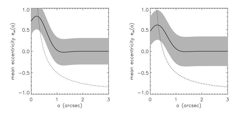
Figure 1: The mean eccentricity $e_{m}(a)$ as a function of semimajor axis, for the aligned (left) and non-aligned (right) models. The gray bands represent 1–$\sigma$ deviations (parameter $\sigma_{e}$). Note that Monte-Carlo points with $|e|>1$ are discarded. The dashed line is the locus of orbits with apoapsis equal to 0 $\farcs$5, the separation of P1 and P2.

To choose the function $g(a)$ that specifies the semimajor axis distribution, we first convert the DF (10) into an effective surface density distribution; here the effective surface density $\Sigma(a)$ is defined so that $2\pi a\Sigma(a)da$ is the mass with semimajor axes in the range $[a,a+da]$. We have

$$\Sigma(a_{0})={1\over 2\pi a_{0}}\int d{\bf J}d{\mbox{\boldmath$\theta$}}\,\delta(a-a_{0})f({\bf J},{\mbox{\boldmath$\theta$}}),$$ (13)

where the action-angle variables $({\bf J},\mbox{\boldmath$\theta$})$ are defined in equation (9). For the DF (10) we have

$$\Sigma(a_{0})={\pi\mu^{3/2}\over a_{0}^{1/2}}g(a_{0})\int_{0}^{\pi}dI\,\sin I\exp\left[-\frac{I^{2}}{2\sigma_{I}(a_{0})^{2}}\right]\int_{0}^{2\pi}d\varpi\int_{0}^{\infty}de\,e\exp\left[-\frac{[{\bf e}-{\bf e}_{m}(a_{0})]^{2}}{2\sigma_{e}^{2}}\right].$$ (14)

The innermost two integrals are easily evaluated by writing $e\,de\,d\varpi=d{\bf e}$ and using Cartesian coordinates for ${\bf e}$:

$$\Sigma(a_{0})={2\pi^{2}\mu^{3/2}\sigma_{e}^{2}\over a_{0}^{1/2}}g(a_{0})\int_{0}^{\pi}dI\,\sin I\exp\left[-\frac{I^{2}}{2\sigma_{I}(a_{0})^{2}}\right].$$ (15)

Since $\sigma_{I}(a_{0})$ is generally small, to a good approximation we have

$$\Sigma(a_{0})=2\pi^{2}\mu^{3/2}\sigma_{e}^{2}\sigma_{I}^{2}(a_{0})a_{0}^{-1/2}g(a_{0}).$$ (16)

Initially, we tried a simple exponential for the effective surface-density distribution, but we found that this form results in too much light at the center, and too much contamination of the bulge by the disk at large radii. After some experimentation, we concluded that to match the photometry we require an effective surface-density distribution that has a central minimum, an outer cut-off, and a maximum roughly at the P1 position. The steepness of the inner gradient of the distribution is important. For example, we experimented with a Gaussian distribution, $\Sigma(a)=\Sigma_{0}\exp[-k(a-a_{0})^{2}]$, and an exponential model with a central hole, $\Sigma(a)=\Sigma_{0}[\exp(-a/a_{0})-\exp(-a/a_{1})]$. We found that for the former distribution the best-fit model (viewed from above the disk) has a wider central hole with a more well-defined boundary, a more well-defined P1 peak which extends for a greater distance around the circumference of the disk, and less surface brightness coming from the outer extremities of the disk. When projected onto the sky plane, the Gaussian model is less successful in reproducing the dip in the surface brightness profile between the P1 and P2 peaks. The fact that the double-exponential model is asymmetric about its maximum also seems to help in reproducing the photometric data. In the case of the double-exponential model, we consistently found best-fit models where $a_{1}\sim a_{0}$, leading to an inner gradient rising as $a$. We also experimented with models with $\Sigma(a)=\Sigma_{0}a^{n}\exp(-a/a_{0})$, and settled on $n=2$ as the most promising value of this parameter. Therefore, we choose the following distribution, with a hole in the middle and an outer Fermi-type cutoff,

$$\Sigma(a)=\Sigma_{0}\frac{a^{2}\exp(-a/a_{0})}{1+\exp\left[c_{1}(a-c_{2})\right]};$$ (17)

the fit is quite insensitive to the value of the cut-off parameter $c_{1}$. We then define $g(a)$ using equation (16).

In total, our model for the DF depends on 10 parameters: two for the semimajor axis distribution ($a_{0}$, $c_{1}$, $c_{2}$); two for the inclination distribution ($\sigma_{I}^{0}$, $a_{I}$), and five for the eccentricity distribution ($\alpha$, $a_{g}$, $a_{e}$, $w$, $\sigma_{e}$).

2.4 The bulge

The M31 bulge is assumed to be spherical, isotropic and non-rotating. This relatively crude model is adequate because the bulge contributes only a modest background correction in the region $R\lesssim 2\arcsec$ that is dominated by the nucleus. We use the photometric parameters of KB99 for our bulge model. At radii $<300\arcsec$, they found that the surface brightness of the bulge is well-described by a Sérsic (1968) law, $I(R)=I_{0}\exp[-(R/R_{n})^{1/n}]$, with $I_{0}=15.40\hbox{ mag arcsec}^{-2}$ in $V$, $R_{n}=14\,\farcs 0$, and $n=2.19$. With this bulge-nucleus decomposition, the central surface brightness of the bulge is 16% of the peak surface brightness of the nucleus.

Much of our analysis will be based on the bulge-subtracted kinematic data of KB99, in which case the bulge kinematics are irrelevant for our models. However, for some purposes we compare the model to kinematic data that includes the bulge light, and in this case we must model the bulge kinematics. To do so, we assume that the bulge has constant mass-to-light ratio $\Upsilon$, compute the gravitational potential of the spherical Sérsic profile described above, and add a central point mass corresponding to the (unknown) total mass of the BH plus nuclear disk. We then solve for the line-of-sight velocity distribution (LOSVD) at each radius, using formulae from Binney & Tremaine (1987) and Simonneau & Prada (1999).

We assume that the mass-to-light ratios $\Upsilon$ of the bulge and nuclear disk are the same; this assumption is unlikely to be completely accurate since the colors of the nucleus and bulge are different, but the model predictions are only weakly dependent on the mass-to-light ratio of the bulge, and the mass-to-light ratio of the disk only affects the model through the displacement between the BH and the bulge center, which is at the center of mass of the BH and the stellar disk.

3 Numerical methods

3.1 Constructing the nuclear disk

We simulate the nuclear disk using a Monte-Carlo method, typically with $N=10^{7}$ particles (there is little point in larger simulations, since $N$ is already comparable to the number of stars in the actual disk, and much larger than the number of giant stars, which dominate the light). First we assign semimajor axes $a$ to the particles so that the distribution is uniform in $\int_{0}^{a}\Sigma(a^{\prime})a^{\prime}\,da^{\prime}$. For a given semimajor axis, the DF (10) implies that the mass in a small interval of the other orbital elements is

$$dm\propto\exp\left[-\frac{[{\bf e}-{\bf e}_{m}(a)]^{2}}{2\sigma_{e}^{2}}\right]\exp\left[-\frac{I^{2}}{2\sigma_{I}(a)^{2}}\right]\,d{\bf e}\sin I\,dI\,dM\,d\Omega.$$ (18)

Thus, for each particle we choose $\Omega$ and $M$ from uniform probability distributions over the range $[0,2\pi)$; $e_{x}$ and $e_{y}$ from Gaussian distributions with means $e_{m}(a)$ and 0 respectively, and standard deviation $\sigma_{e}$; and $I$ from a Gaussian distribution weighted by $\sin I$, with standard deviation $\sigma_{I}(a)$. We obtain the eccentric anomaly $E$ by numerical solution of Kepler’s equation [the third of equations (5)]. We then use equations (5) and (6) to determine the position $(x^{\prime},y^{\prime},z^{\prime})$ and velocity $(\dot{x}^{\prime},\dot{y}^{\prime},\dot{z}^{\prime})$, and equations (3) and (4) and their time derivatives to determine the positions and velocities in the sky-plane coordinate system.

3.2 Photometry

We fit the model to the deconvolved HST V-band (F555W) image presented in L98. The intensity scale is calibrated using the zero-point given in L98. We assume that the pixel containing the maximum luminosity in the blue cluster in the P2 peak is the position of the BH, and this point is also the origin of our coordinate systems. The excess brightness contributed by the UV cluster at P2 in the data is clipped out prior to fitting, since we may assume that these stars have a small mass-to-light ratio. We compare the data to the model on a sky-plane grid with cell size equal to the pixel size, $0\,\farcs 0228=0.085\hbox{\, pc}$, and a circular boundary of radius $R_{g}=5\hbox{\, pc}=1\,\farcs 34$.

We add the surface-brightness contribution from the bulge by assuming that the center of the bulge coincides with the center of mass of the disk-BH system; thus the center of the bulge is not precisely at the origin.

3.3 Kinematics

We fit the kinematics to the bulge-subtracted spectroscopic data from KB99, which combine high S/N with reasonably good spatial resolution. These data have a scale of 0 $\farcs$0864/pixel, a PSF with FWHM of 0 $\farcs$64, and a slit width $2s=0\,\farcs 35$. Two spectra were taken at position angle $\hbox{PA}=50\arcdeg$ and two more at $\hbox{PA}=55\arcdeg$. KB99 then shifted these four spectra to a common center and co-added them for further analysis.

We reproduce this procedure in the model. We compute the LOSVD from the nucleus on a sky-plane grid with cell size equal to the pixel size, and then smooth the LOSVDs by convolving with the PSF given in equation (3) of KB99 and a top-hat slit of width $2s$. We then add the LOSVDs at $\hbox{PA}=50\arcdeg$ and $\hbox{PA}=55\arcdeg$. Following KB99, we fit the LOSVDs with a fourth-order Gauss-Hermite expansion (van der Marel & Franx, 1993; Gerhard, 1993):

$${\mathrm{LOSVD}}(v)=\frac{\gamma}{\sqrt{2\pi\sigma^{2}}}e^{-(v-V)^{2}/2\sigma^{2}}\left[1+h_{3}H_{3}\left(\frac{v-V}{\sigma}\right)+h_{4}H_{4}\left(\frac{v-V}{\sigma}\right)\right].$$ (19)

The coefficients $h_{3}$ and $h_{4}$ parametrize the lowest order odd and even deviations from Gaussian line profiles. The velocity bins are $5\hbox{\,km s}^{-1}$ wide and are weighted equally in the fit. The kinematic parameters extracted from the fit ($V,\sigma,h_{3},h_{4}$) can then be compared with the observations from KB99.

3.4 Parameter fitting

We fit the sky-plane image to the model using the statistic

$$\chi_{1}^{2}=\sum_{R\leq R_{g}}w(i,j)\left[\mathrm{datagrid}(i,j)-\mathcal{A}\ \mathrm{modelgrid}(i,j)\right]^{2},$$ (20)

where $\mathcal{A}$ specifies the overall normalization of the model, $w(i,j)$ is the weight assigned to pixel $(i,j)$, and $R_{g}$ is the radius of the region we are fitting.

One potential drawback of this approach is that most of the weight comes from the outer parts of the image, while the most critical photometric test of the model is its ability to fit the observations near the center, in particular along the P1-P2 axis. We have addressed this problem in two ways: (i) we have used a weight function $w(i,j)=\sqrt{\mathrm{datagrid}(i,j)}$, which gives more weight to the high-surface brightness regions in P1 and P2 (the form of this weighting factor was selected after experimenting with a variety of possibilities). (ii) We have computed a second statistic, $\chi_{2}^{2}$, which is similar to $\chi_{1}^{2}$ but restricted to pixels in a slit (of width one pixel on the model photometric grid) that extends through P1 and P2 to a distance $\pm R_{g}$ from the origin. This statistic focuses on the difficult task of fitting the double structure of the nucleus.

We specify the fit to the kinematic data by a statistic $\chi_{3}^{2}$, which measures the mean-square differences of $V$ and $\sigma$ between the model and the KB99 bulge-subtracted data at 46 points along the PA=50°–55°axis (Table 3 of KB99). Each data point is weighted by the observational uncertainty given by KB99. Note that KB99 present velocity and dispersion measurements extracted with two techniques: Fourier Quotient (FQ, their Tables 2 and 3) and Fourier Correlation Quotient (FCQ, their Tables 4 and 5). The Gauss-Hermite fitting procedure outlined above mimics the FCQ algorithm more closely; however, the FQ data are given at significantly finer spatial resolution. The velocity differences between the two algorithms are $\leq 2$ km s^-1; the close agreement between the two sets of velocity and dispersion data is illustrated in Figures 5 and 6. Thus we choose to fit to the KB99 FQ data.

We determine the best-fit model by minimizing the statistic $\chi_{1}^{2}+\lambda_{1}\chi_{2}^{2}+\lambda_{3}\chi_{3}^{2}$, where the relative weights $\lambda_{1}$ and $\lambda_{2}$ are chosen by hand such that for the initial state model for the full photometry and kinematics fit, $\chi_{1}^{2}\sim\lambda_{1}\chi_{2}^{2}$ and $(\chi_{1}^{2}+\lambda_{1}\chi_{2}^{2})\sim\lambda_{3}\chi_{3}^{2}$. The procedure used to determine the initial state model is described later in this section.

We do not fit to KB99’s measurements of the Gauss-Hermite parameters $h_{3}$ and $h_{4}$, or to spectroscopic data from other investigators. However, we shall compare the best-fit models we obtain in this way to STIS observations of kinematic parameters including $h_{3}$ and $h_{4}$.

To reduce the dimensionality of our large parameter space, we choose two parameters by hand: $c_{1}$ and $\Upsilon=M/L_{V}$. The Fermi cut-off parameter $c_{1}$ (eq. 17) does not significantly affect the fit within the inner 2″, and the photometry is quite insensitive to its exact value, so we simply choose $c_{1}=4\hbox{\, pc}^{-1}$. The mass-to-light ratio $\Upsilon$ does not enter the kinematic fit since we use bulge-subtracted kinematic data, and only affects the photometric fit through the displacement between the BH and the bulge center, which is the barycenter of the BH and nuclear disk. To find the position of the barycenter, we simply assume the same mass-to-light ratio for the nuclear stars as the KB99 value for the bulge stars, $\Upsilon_{V}=5.7$. We then use the resulting disk mass and the model’s BH mass to compute the position of the barycenter.

If the nuclear disk is assumed to be aligned with the M31 disk (“aligned models”) we now have 11 free parameters: one orientation parameter ($\theta_{a}$, the angle in the disk plane between the sky plane and the symmetry axis of the nuclear disk); one mass parameter (the BH mass $M_{\bullet}$), and 9 parameters for the disk DF ($a_{0},c_{2},\sigma_{I}^{0},a_{I},\alpha,a_{g},a_{e},w,\sigma_{e}$). If the nuclear disk orientation is fitted to the data (“non-aligned models”), we must fit two more orientation parameters, $\theta_{i}$ and $\theta_{l}$.

The fitting is done with a downhill simplex algorithm (Press et al., 1992).

To obtain initial conditions for the fitting program, we made use of the thin disk model. It is relatively easy to find parameters for equations (12) and (17) that give a thin disk $x$-axis surface-brightness profile (1) similar to the observed profile along the P1-P2 axis. Hence, reasoning that thickening the disk would lower the surface brightness at P1, we chose as a starting point an “extreme” thin disk model which maximized the ratio of surface brightnesses P1/P2.

This extreme thin disk model produced optimum values for the parameters [$a_{0},a_{1},\alpha,a_{g},a_{e},w$]. These were then used as a first guess to fit to the photometry of the three-dimensional disk model (using only the statistic $\chi_{1}$), with plausible initial guesses for $a_{I}$, $\theta_{a}$, $\sigma_{I}^{0}$ and $\sigma_{e}$. When the fitting algorithm converged for this limited parameter set, they were then input into the full kinematic and photometric fit as an initial guess, adding $M_{\bullet}$ to the fit.

It should be emphasized that the thin disk model was only used to obtain the initial conditions; the rest of the fitting process uses the thick disk model of §2.

4 Results

Figure 2: Surface-brightness distribution in the nucleus of M31. The left panel shows the data (V-band; from L98) and the right panel shows the best aligned model. Contours are at 0.25 mag intervals. North is $55.7\arcdeg$ to the left of the top of the plot.

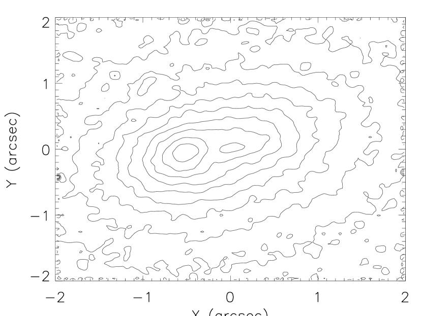
Figure 3: Surface-brightness distribution in the nucleus of M31. The left panel shows the data (V-band; from L98) and the right panel shows the best non-aligned model. Contours are at 0.25 mag intervals. North is $55.7\arcdeg$ to the left of the top of the plot.

Figure 4: Surface brightness along a slit of width 1 pixel ($=0\,\farcs 0228$) that extends through P1 and P2. The solid line represents the data (from L98) and the dashed lines are the best aligned model (left panel) and non-aligned model (right panel).

Figure 5: Rotation speed $V$ along the axis at PA=50$\arcdeg$–55$\arcdeg$, as determined by fitting the LOSVD to the Gauss-Hermite expansion (19). The data from KB99 after bulge subtraction are shown as black dots (FCQ) and crosses (FQ), and the solid lines are the best aligned model (left panel) and non-aligned model (right panel).

Figure 6: The dispersion $\sigma$ along the axis at PA=50$\arcdeg$–55$\arcdeg$, as determined by fitting the LOSVD to the Gauss-Hermite expansion (19). The data from KB99 after bulge subtraction are shown as black dots (FCQ) and crosses (FQ), and the solid lines are the best aligned model (left panel) and non-aligned model (right panel).

Figure 7: The Gauss-Hermite parameter $h_{3}$ along the axis at PA=50$\arcdeg$–55$\arcdeg$. The data from KB99 after bulge subtraction are shown as black dots (FCQ), and the solid lines are the best aligned model (left panel) and non-aligned model (right panel).

Figure 8: The Gauss-Hermite parameter $h_{4}$ along the axis at PA=50$\arcdeg$–55$\arcdeg$. The data from KB99 after bulge subtraction are shown as black dots (FCQ), and the solid lines are the best aligned model (left panel) and non-aligned model (right panel).

Table 1: Model parameters

parameter	aligned model	non-aligned model
$\alpha$	0.288	0.197
$a_{e}$ (pc)	3.97	4.45
$a_{g}$ (pc)	1.51	1.71
$w$ (pc)	1.53	1.52
$M_{\bullet}(M_{\odot})$	$9.63\times 10^{7}$	$1.02\times 10^{8}$
$a_{0}$ (pc)	4.61	1.37
$c_{1}$ (pc-1)	4	4
$c_{2}$ (pc)	3.79	4.24
$\sigma_{e}$	0.344	0.307
$\theta_{a}$ (deg)	$-11.0$	$-34.5$
$a_{I}$ (pc)	13.7	31.5
$\sigma_{I}^{0}$ (deg)	36.2	24.6
$\theta_{i}$ (deg)	77.5	54.1
$\theta_{l}$ (deg)	$-52.3$	$-42.8$
$\Upsilon(M_{\odot}/L_{\odot})$	5.7	5.7

Table 2: Model photometry

parameter	A	N	data
Separation of P1 and P2 (arcsec)	0.6	0.5	0.5 (L98)
P1–P2 position angle (deg)	$39\arcdeg$	$42\arcdeg$	$43\arcdeg$
Separation of P2 from bulge center (arcsec)	0.04	0.04	0.07 (KB99)
Disk luminosity $\leq 1\arcsec$ projected ($L_{\odot}$)	$2.9\times 10^{6}$	$2.9\times 10^{6}$	$2.9\times 10^{6}$
Disk luminosity inside $4\arcsec\times 4\arcsec$ box ($L_{\odot}$)	$3.6\times 10^{6}$	$3.6\times 10^{6}$	$5.4\times 10^{6}$

Note. — A=aligned model; N=non-aligned model. Disk luminosity is computed using bulge model from KB99. The projected model disk luminosity is normalized to the projected bulge-subtracted data luminosity $\leq 1\arcsec$.

Table 3: Model kinematics

parameter	A,S	N,S	STIS (FCQ)	A,K	N,K	KB99 (FQ)
P1 rotation maximum (km s-1)	193	198	203	170	178	179
Position of rotation maximum (arcsec)	$-0.76$	$-0.61$	$-0.59$	$-0.95$	$-0.86$	$-0.99$
Anti-P1 rotation minimum (km s-1)	$-277$	$-369$	$-319$	$-212$	$-228$	$-236$
Position of rotation minimum (arcsec)	0.41	0.20	0.25	0.78	0.60	0.65
$V=0$ position (arcsec)	$-0.17$	$-0.12$	$-0.12$	$-0.05$	$-0.05$	$-0.05$
Dispersion peak (km s-1)	252	328	302	248	274	287
Position of dispersion peak (arcsec)	0.15	0.10	0.08	0.17	0.09	0.13

Note. — A=aligned model; N=non-aligned model; K=KB99 resolution; S=STIS resolution

We shall describe two models: the best-fit aligned model, in which the nuclear disk is assumed to lie in the symmetry plane of the M31 disk, and the best-fit non-aligned model, in which the orientation of the nuclear disk is chosen to optimize the fit.

The aligned model we describe here was obtained by minimizing the statistic $\chi_{1}^{2}/(6\times 10^{6})+\chi_{2}^{2}/(6\times 10^{4})+\chi_{3}^{2}$, while the non-aligned model was based on the statistic $\chi_{1}^{2}/(1.2\times 10^{7})+\chi_{2}^{2}/(1.2\times 10^{5})+\chi_{3}^{2}$. The parameters of the models are given in Table 1.

Figures 2 and 3 show the surface-brightness distributions in the data and the two models. Both models correctly reproduce the apparent double structure of the nucleus, and the approximate sizes and shapes of P1 and P2. However, in the aligned model the maximum surface brightness of P1 is lower than the maximum brightness in P2, while in the observations P1 is brighter. The non-aligned model does much better in reproducing the relative surface brightnesses of P1 and P2.

The position angle of the line joining P1 and P2 is $39\arcdeg$ in the aligned model and $42\arcdeg$ in the non-aligned model, close to the observed value of $43\arcdeg$. The position angle of the major axis of P1 in the data (as determined by the isophotes with semimajor axis less than 0 $\farcs$2) is $63\arcdeg$. This $20\arcdeg$ isophote twist is not reproduced in the models. However, the observed twist is strongly affected by the limited number of giant stars that contribute to the surface brightness in the middle of P1. We have explored this effect by reducing the number of stars in our Monte-Carlo realization by a factor $\sim 100$ to approximate the actual number of giants in the nucleus (of order $10^{5}$). We find that in this case the position angle of the P1 major axis varies significantly in different realizations; therefore, the difference in position angle between the major axis of P1 and the P1-P2 axis does not provide much useful information. However, the range of position angles seen in realizations of the non-aligned model is larger than in the aligned model, so that the non-aligned model is more easily able to accommodate the $20\arcdeg$ isophote twist seen in the data.

Figure 4 shows the surface brightness along the P1-P2 axis in both models. In the data, the surface-brightness peak at P1 is approximately 0.4 mag brighter than the peak at P2. In the aligned model, P1 is fainter than P2 by 0.1 mag, while in the non-aligned model P1 is brighter by 0.2 mag; thus the fit of the non-aligned model to the relative brightnesses of P1 and P2, though not perfect, is much better than the aligned model. The brightness of P1 can be increased in the aligned model by reducing the disk thickness (smaller $\sigma_{I}^{0}$) but then P1 becomes too elongated.

The non-aligned model correctly reproduces the dip in surface brightness between P1 and P2, but the minimum is displaced 0 $\farcs$2 further toward P2 than it is in the data. A feature of both models is that the P2 peak is displaced to the anti-P1 side of the our origin at the BH (i.e. the UV peak P2B). This is a consequence of the luminosity depression imposed at the origin ($\Sigma(a)\propto a^{2}$, eq. 17). While in principle this displacement could be an important test of the model, with implications for the kinematics (specifically, the displacement of the dispersion peak to the anti-P1 side), we have found that this displacement cannot be determined reliably if the number of stars in the simulation is reduced to approximate the number of giant stars in the actual system: in this case Monte-Carlo simulations can be created which have no significant displacement of the P2 peak from P2B.

Note that both models fail to reproduce the surface brightness outside $\sim 1\,\farcs 3$, because the surface brightness in the model falls off more sharply than in the data. The obvious fix is to increase the cutoff parameter $c_{2}$ in equation (17). However, this change affects the fit to the kinematics, decreasing the amplitude of the rotation minimum and lowering the dispersion peak. The discrepancy in the surface brightness at large radii could arise either because the real bulge is cuspier than our model, which we adopted from KB99, or because the nucleus contains extended wings that are not captured by our parametrization.

Figure 5 shows the rotation speed $V$—more precisely, the parameter $V$ in the Gauss-Hermite expansion (19)—along the average of the two slits at PA=50$\arcdeg$ and 55$\arcdeg$ measured in KB99. The aligned model, shown in the left panel, reproduces the approximate shape of the rotation curve, in particular the strong asymmetry (the peak of the observed rotation curve is at $179\hbox{\,km s}^{-1}$ on the P1 side and $236\hbox{\,km s}^{-1}$ on the anti-P1 side; see Table 3 for the peak velocities in the models). The zero-point of the model rotation curve is displaced from P2B toward P1 by $0\,\farcs 05$, consistent with the displacement of 0 $\farcs$05–0 $\farcs$10 estimated by KB99. The most significant discrepancy is that the maximum rotation speed on the anti-P1 side, near 0 $\farcs$6, is too small by about $24\hbox{\,km s}^{-1}$ or 10%; the rotation speed near the peak on the P1 side is also too low, but by a smaller amount.

The right panel shows the rotation curve for the non-aligned model, which fits the rotation curve substantially better than the best aligned model.

Figure 6 shows the dispersion profile along the same slits. The dispersion profile in the aligned model, shown on the left, fits the data fairly well, but (i) the maximum dispersion is too low by 14% ($248\hbox{\,km s}^{-1}$ compared to $287\hbox{\,km s}^{-1}$); (ii) the model dispersion is too large by about $10\hbox{\,km s}^{-1}$ on the P1 side between radii of 0 $\farcs$4 and 1 $\farcs$1. The dispersion is also too high near 2″ on the anti-P1 side, but this discrepancy probably is due to the shortcomings of the bulge model discussed above.

The model correctly reproduces the displacement of the dispersion peak from P2B by about 0 $\farcs$13 in the anti-P1 direction—the displacement in the model is about 0 $\farcs$17. We could increase the peak dispersion in the model by increasing the BH mass, but then the excess model dispersion on the P1 side would become even worse.

We have attempted to increase the maximum dispersion by adding a compact spherical stellar system at P2 (in the form of a Plummer sphere); the hope was that the high-velocity stars in a small, low-luminosity system of this kind would increase the dispersion without degrading the fit to the photometry. However, we found that increasing the dispersion profile in this manner made the rotation curve too symmetrical, so the overall fit was not improved.

The dispersion profile and rotation curve of the aligned model could be made to fit the KB99 data if we assume that the width of the PSF is 10–15% smaller than the value used by KB99. However, it is unlikely that there is an error of this magnitude in the estimated PSF.

The right panel of Figure 6 shows the dispersion profile in the non-aligned model. The model profile fits the data substantially better than the best aligned model, though the maximum dispersion is still too low by 5%. The dispersion peak is displaced by 0 $\farcs$09 from P2B in the anti-P1 direction, in good agreement with the observed displacement of 0 $\farcs$13.

Figures 7 and 8 show the parameters $h_{3}$ and $h_{4}$ in the Gauss-Hermite expansion. Both the aligned and non-aligned models are moderately successful at reproducing the data within the large uncertainties; thus it appears that a model that is fit to the overall scale and center of the velocity distribution (measured by $\sigma$ and $V$) also reproduces the gross features of its shape. Note that we do not use data on either $h_{3}$ or $h_{4}$ in the fitting process, so the comparisons in these figures are a measure of the predictive power of the eccentric-disk model rather than the quality of the fit.

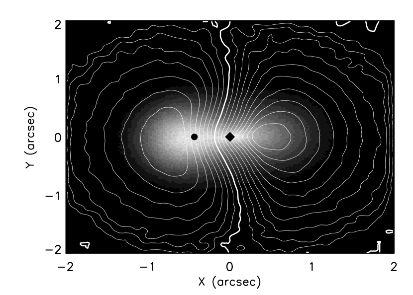
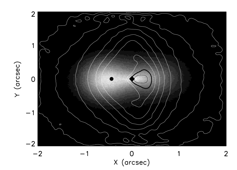
Figure 9: Two-dimensional kinematics of the best aligned model. The left panel shows the mean-velocity contours and the right panel shows the velocity-dispersion contours; both panels are superimposed on a gray-scale image of the nucleus. The contour interval is $25\hbox{\,km s}^{-1}$. The thick line is the zero (systemic) velocity contour (left panel) and the $200\hbox{\,km s}^{-1}$ dispersion contour (right panel). The locations of the center of P1 (filled circle) and P2B (filled diamond at the origin) are shown. North is $55.7\arcdeg$ to the left of the top of the plot.

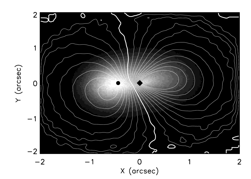
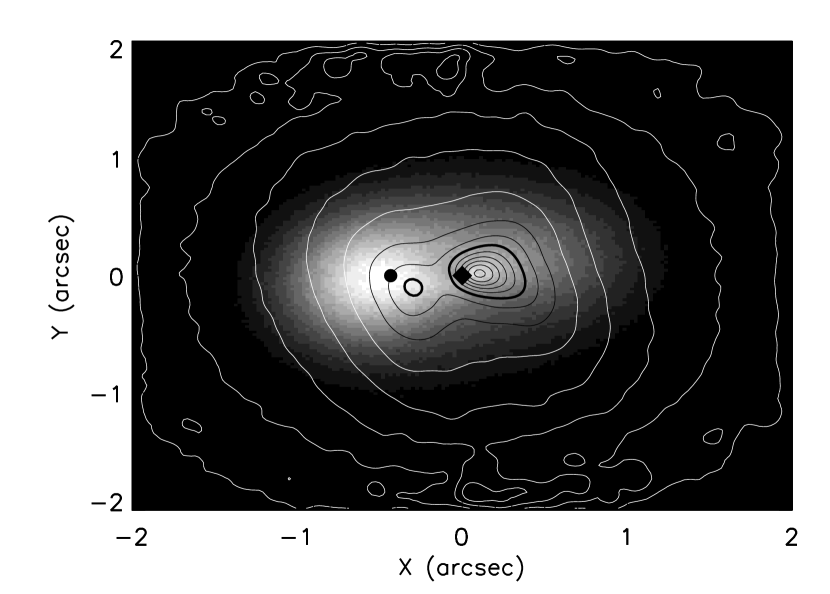
Figure 10: Two-dimensional kinematics of the best non-aligned model. Parameters as in Figure 9.

B01 have used the OASIS integral-field spectrograph, assisted by adaptive optics, to measure the two-dimensional mean-velocity and velocity-dispersion fields in the central 1 $\farcs$5 of M31, with a PSF having FWHM of $\sim$0 $\farcs$4–0 $\farcs$5. They find that the kinematic axis (the axis of symmetry of the mean-velocity field) has a position angle of $56\arcdeg$, which is rotated from the P1–P2 axis at position angle $43\arcdeg$. Figures 9 and 10 show the mean-velocity and velocity-dispersion fields for the aligned and non-aligned models, as viewed with a Gaussian PSF having FWHM of 0 $\farcs$13 to smooth out the shot noise in the contours. These figures can be directly compared to the model photometry in Figures 2 and 3, which has the same resolution and orientation. Once again, the non-aligned model provides a better fit to the data than the aligned model. In particular, the kinematic major axis (defined by the line joining the velocity extrema) in the non-aligned model has PA=48–50$\arcdeg$, much closer to the observed orientation of $56\arcdeg$ than the kinematic major axis in the aligned model, PA=40$\arcdeg$. We suspect that the orientation of the kinematic axis is resolution-dependent, which may account for the difference of $7\arcdeg$ between the non-aligned model and the B01 data. In Figure 7 of B01, the isovelocity contours between P1 and P2 are nearly perpendicular to the line joining the velocity extrema, while this angle is oblique in our non-aligned model. We find that lower-resolution maps of the velocity field of the non-aligned model yield isovelocity contours that are more nearly perpendicular to the kinematic axis, consistent with the B01 data.

4.1 Comparison with STIS data

We now compare the predictions of the models described above to new high-resolution STIS observations (Bender et al., 2003). Recall that our models were fitted to the ground-based spectroscopic data from KB99; here, the kinematics have simply been recomputed for STIS resolution (slit width 0 $\farcs$1) without modifying the fit. The effects of the instrumental broadening on the LOSVD have been accounted for using a template star observed through the same slit (R. Bender, private communication). We use the PSF given by Bower et al. (2001), which can be modeled as the sum of two Gaussians (K. Gebhardt, private communication):

$$G(r)=1.01\exp\left[-\frac{r^{2}}{2(0.0329)^{2}}\right]+0.12\exp\left[-\frac{(r-0.105)^{2}}{2(0.0384)^{2}}\right],$$ (21)

where $r$ is the distance in arcseconds. Note that a Wiener filter has been applied to the STIS data (R. Bender, private communication) to remove high frequencies, a step that we have not taken in analyzing the model kinematics.

The spatial resolution of the STIS observations is far better than that of the KB99 observations (the slit width is a factor of 3.5 smaller, and the FWHM of the PSF is smaller by a factor of 5.4). Thus the comparison of the STIS kinematics with our models is a stringent test of their predictive power.

The kinematics of the best-fit aligned and non-aligned models that would be observed with STIS resolution are shown in Figures 11–14. The solid curves are bulge-subtracted and the dashed curves include the bulge. The data, shown as dots (FCQ) and crosses (FQ), are obtained at PA=$39\arcdeg$ and are bulge-subtracted.

In contrast to the KB99 data, the FQ and FCQ results are substantially different for the STIS data. The difference arises because FQ assumes Gaussian LOSVDs while FCQ simultaneously derives velocities, dispersions, $h_{3}$, and $h_{4}$ by fitting the LOSVD with a Gauss-Hermite series. Thus, the results from the two techniques do not agree where LOSVDs have strong wings and the higher order Gauss-Hermite moments are large. Since we mimic the FCQ procedure in our calculations, one should compare the model curve with the FCQ results (the dots).

The non-aligned model is remarkably successful at reproducing the rotation curve on the P1 side, as well as the rotation gradient through the center (right panel of Fig. 11). On the anti-P1 side the peak rotation speed in the model is too high by 16% (see Table 3) and the model rotation curve outside the peak is also too high.

The displacement of the zero of the rotation curve is 0 $\farcs$12 toward P1 in both the data and the non-aligned model.

The dispersion peak in the non-aligned model is 9% too high (Fig. 12). The dispersion peak position is reproduced correctly—in the data the peak is displaced in the anti-P1 direction by 0 $\farcs$08, compared to 0 $\farcs$10 in the model.

At this resolution, both models show a secondary peak in the dispersion curve (Fig. 12). This peak is a consequence of the hole in the middle of the model surface density distribution. The data do not conclusively favor or disfavor a feature at this location. One can possibly make this feature less prominent by making the central surface-brightness gradient shallower. However, we have been unable to remove the central hole completely without drastically worsening the fit to the photometry. Thus, we believe that a secondary peak in the dispersion profile should generally be present at some level in the type of model proposed here.

The model dispersions are much lower than the dispersions in the data at radii around $1\arcsec$. We believe that this discrepancy arises because the KB99 bulge model and our disk model do not have enough flexibility to match the photometry and kinematics in this region; however, this problem should not affect our models at smaller radii.

Both the aligned and non-aligned models are quite successful in reproducing the overall shape of the profiles of the Gauss-Hermite parameters $h_{3}$ and $h_{4}$ (Figs. 13 and 14). In particular, the models reproduce the shape, amplitude, and location of the sharp dip in $h_{3}$ and the peak in $h_{4}$. The agreement between data and models is particularly impressive since the model is derived by fitting only to the low-resolution mean velocity and dispersion profiles.

Figure 15 shows the LOSVDs for each model at a few locations near P2. These LOSVDs are calculated at STIS resolution along PA=$39\arcdeg$, and do not include the bulge. Near the BH, the LOSVDs are very asymmetric and have strong wings on the prograde side of the mean rotation velocity. These features are also seen in the STIS LOSVDs (plotted here in long dashes). However the model wings are more extensive than in the data.

Note that the model LOSVDs are constrained to be positive, while the STIS LOSVDs are not; thus the latter show (unphysical) low-amplitude oscillations that are not present in the models.

Figure 11: Rotation speed $V$ along the axis at PA=39$\arcdeg$, as observed with STIS resolution (see text). The rotation speed is determined by fitting the LOSVD to the Gauss-Hermite expansion (19). The best aligned model is shown in the left panel and the best non-aligned model is shown in the right panel. The solid curve is bulge-subtracted and the dashed curve includes the bulge. The bulge-subtracted STIS data from Bender et al. (2003) are shown as black dots (FCQ) and crosses (FQ).

Figure 12: Velocity dispersion $\sigma$ along the axis at PA=39$\arcdeg$, as observed with STIS resolution (see text), determined by fitting the LOSVD to the Gauss-Hermite expansion (19). The best aligned model is shown in the left panel and the best non-aligned model is shown in the right panel. The solid curve is bulge-subtracted and the dashed curve includes the bulge. The bulge-subtracted STIS data from Bender et al. (2003) are shown as black dots (FCQ) and crosses (FQ).

Figure 13: The Gauss-Hermite parameter $h_{3}$ along the axis at PA=39$\arcdeg$, as observed at STIS resolution. The best aligned model is shown in the left panel and the best non-aligned model is shown in the right panel. The solid curve is bulge-subtracted and the dashed curve includes the bulge. The bulge-subtracted STIS data from Bender et al. (2003) are shown as black dots (FCQ).

Figure 14: The Gauss-Hermite parameter $h_{4}$ along the axis at PA=39$\arcdeg$, as observed at STIS resolution. The best aligned model is shown in the left panel and the best non-aligned model is shown in the right panel. The solid curve is bulge-subtracted and the dashed curve includes the bulge. The bulge-subtracted STIS data from Bender et al. (2003) are shown as black dots (FCQ).

Figure 15: The LOSVD distributions near P2 at STIS resolution for the aligned (dotted) and non-aligned (solid) models. The LOSVDs from the STIS data are plotted in long dashes (in places the STIS LOSVD is negative and these sections are not shown). The curves are normalized to unit area. The velocity zero point is the systemic velocity of M31. Note that not all the LOSVD bins have the STIS LOSVDs overplotted, because they were provided only at specific radii, and we could only match some of these radii to a corresponding pixel on our LOSVD grids.

4.2 Internal dynamics of the disk

T95 suggested that two-body relaxation would lead to significant thickening of a thin disk if the disk age were comparable to the Hubble time. In this subsection we investigate this process quantitatively for our disk models. For simplicity, we shall neglect the mean eccentricity of the disk, that is, we approximate the disk as axisymmetric.

Axisymmetric gravitational stability in a razor-thin disk requires that Toomre’s $Q$ parameter exceeds unity, where (Toomre, 1964; Binney & Tremaine, 1987)

$$Q\equiv 0.30\sigma_{e}{M_{\bullet}\over\Sigma(a)a^{2}};$$ (22)

here $\Sigma(a)$ is the surface density at radius $a$ and $\sigma_{e}$ is the rms value of one component of the eccentricity vector or $2^{-1/2}$ of the rms scalar eccentricity. Using the surface-density distributions in the aligned and non-aligned models, we find that the value of $\sigma_{e}$ required for stability never exceeds 0.1 (Fig. 16); once the non-zero disk thickness is included, the required value would be even lower. Thus the aligned and non-aligned disk models, which have $\sigma_{e}=0.34$ and $0.31$, are safely stable.

Let us assume that the disk formed $t_{0}=1\times 10^{10}\hbox{\,yr}$ ago, and was initially cold (i.e. $\sigma_{e}$ just large enough for gravitational stability). Two-body relaxation will gradually increase both the rms eccentricity and the rms inclination of the disk stars. This process of “disk heating” or “viscous stirring” has been studied thoroughly in protoplanetary disks. It is found that disk heating leads to a specific ratio between the rms inclination and eccentricity, $\sigma_{I}\simeq 0.5\sigma_{e}$, and that (Ohtsuki, Stewart, & Ida, 2002)

$$\langle I^{2}\rangle^{2}(t_{0})=4.52\Omega t_{0}{\Sigma(a)a^{2}\over M_{\bullet}}{m_{*}\over M_{\bullet}}\ln\Lambda,\qquad\Lambda=0.6{M_{\bullet}\over m_{*}}\langle I^{2}\rangle^{3/2};$$ (23)

where $\langle I^{2}\rangle=2\sigma_{I}^{2}$ is the mean-square inclination, $\Omega(a)=(GM_{\bullet}/a^{3})^{1/2}$, and $m_{*}$ is the stellar mass. In deriving this formula we have neglected the time variation of $\langle I^{2}\rangle$ in the factor $\Lambda$, since it only appears in a logarithm, and we have assumed that the disk is in the dispersion-dominated regime, where $\langle I^{2}\rangle^{1/2}\gg(m_{*}/M_{\bullet})^{1/3}\simeq 0.002$.

Figure 16: The inclination and eccentricity dispersions $\sigma_{I}$ (solid lines) and $\sigma_{e}$ (dashed lines) in the aligned model (left panel) and the non-aligned model (right panel). The quantities $2\sigma_{I}^{2}$ and $2\sigma_{e}^{2}$ are the mean-square inclination and eccentricity at a given semimajor axis in a disk with mean eccentricity ${\bf e}_{m}=0$. Also shown are the dispersions expected from two-body relaxation if the disk age is $10^{10}\hbox{\,yr}$, from equation (23) and the relation $\sigma_{I}=0.5\sigma_{e}$. The curve labeled $\sigma_{e}(Q=1)$ is the minimum eccentricity dispersion required for axisymmetric gravitational stability (eq. 22).

The predicted eccentricity and inclination dispersions, $\sigma_{I}=\langle I^{2}\rangle^{1/2}/\surd{2}$ and $\sigma_{e}=2\sigma_{I}$, are shown in Figure 16 for the aligned and non-aligned models. We have shown both the theoretical predictions derived from equation (23) and the surface density and BH mass from Table 1, and our empirical fits to the eccentricity and inclination dispersions, also from Table 1. Note that the theoretical predictions should be robust, since the predicted value of $\sigma_{I}$ depends on only the fourth root of the age, surface density, stellar mass, etc. (eq. 23); the principal uncertainty is probably our assumption that the disk is axisymmetric.

Two-body relaxation requires that the disk axis ratio in the radius range 0.5–$1\arcsec$ is at least 0.13–0.17 in the aligned model, and 0.23–0.25 in the non-aligned model (these values are $\sigma_{I}$, which equals the ratio $\langle z^{2}\rangle^{1/2}/r$ in a circular disk). In the aligned model, the thickness required by relaxation is much smaller than the model thickness ($\sigma_{I}=0.58$–0.55 in the same radius range), and thinner disks are strongly excluded by the photometry. Thus, if this model is correct, some process other than two-body relaxation must determine the thickness. The non-aligned model is thinner, $\sigma_{I}=0.38$–0.41, and the predicted thickness due to relaxation is larger, so it is possible that in this case the thickness is largely determined by two-body relaxation. In aligned disks there is good agreement between the eccentricity dispersion $\sigma_{e}$ due to relaxation and the best-fit value in the model, while in the non-aligned model the eccentricity dispersion due to relaxation actually exceed the best-fit value in the model. We suspect that these disagreements are consistent with the uncertainties in the model.

5 Discussion

The extremely short dynamical time ($1.5\hbox{\, pc}/200\hbox{\,km s}^{-1}\simeq 7500\hbox{\,yr}$) of the M31 nucleus strongly suggests that it is in dynamical equilibrium, an assumption that we adopt throughout this paper. The M31 nucleus reveals by far the richest phenomenology of any equilibrium stellar system, and hence provides a unique challenge for stellar dynamics.

We have fitted parametrized eccentric-disk models of collisionless stellar systems to the photometry and kinematics of the nucleus. These models explain most of the features in the nucleus successfully. However, despite the large number (11–13) of free parameters and our efforts to use plausible fitting functions for the DF, there remain significant differences between our best-fit models and the observational data: for example, we are unable to fit precisely the separation and relative surface brightnesses of the P1 and P2 components (Fig. 4). The important question of whether these discrepancies arise from shortcomings of the eccentric-disk hypothesis, approximations in our model (e.g. the orbits are assumed to be Keplerian), the limited number of bright stars in the nucleus, or the limited flexibility of our parametrization remains to be determined.

The best-fit black-hole mass is $1.0\times 10^{8}M_{\odot}$ (Table 1); this estimate is likely to be about 10%–20% too high because we have neglected the contribution of the nuclear disk stars to the total mass [the ratio of the disk mass inside $1\arcsec$ to the BH mass is $\sim 0.15$ (Table 2)]. Previous estimates of the BH mass include 3–$7\times 10^{7}M_{\odot}$ (Dressler & Richstone, 1988), $10^{6.5}$–$10^{8}M_{\odot}$ (Kormendy, 1988), 4–$5\times 10^{7}M_{\odot}$ (Richstone, Bower & Dressler, 1990), $7\times 10^{7}M_{\odot}$ (Bacon et al., 1994), $7.5\times 10^{7}M_{\odot}$ (T95), 7–$10\times 10^{7}M_{\odot}$ (Emsellem & Combes, 1997), $(3\pm 1.5)\times 10^{7}M_{\odot}$ (KB99), and $(7{+1.5\atop-3.5})\times 10^{7}M_{\odot}$ (B01). The relatively small mass preferred by KB99 is found by a quite different method than the other estimates (they use the displacement between P2B and the center of the bulge, as opposed to the rotation curve and velocity dispersion profile), and may be subject to systematic errors despite the great care taken by KB99 to measure this small displacement accurately. For comparison, the correlation between BH mass and bulge dispersion observed in other nearby galaxies (Tremaine et al., 2002) predicts a mass of $6\times 10^{7}M_{\odot}$ with an uncertainty of a factor of two.

Although the models presented in this paper represent a substantial advance in accuracy and realism, they still have many shortcomings.

• We assume that the stars in the nuclear disk orbit in the point-mass potential of the BH, that is, we neglect the gravitational forces from the disk and bulge. Neglecting the bulge is reasonably safe: within $1\arcsec$ the mass of the bulge is $<10^{6}M_{\odot}$, less than 1% of the mass of the BH. Neglecting the disk is a more serious approximation: in our best-fit models, the disk mass within $1\arcsec$ is $\sim 15$% of the BH mass (Tables 1 and 2); thus the effects of the self-gravity of the disk are small but not negligible. Including the gravitational potential of the disk will modify the kinematics of the disk orbits, and may permit new types of orbit family not present in the spherically symmetric BH potential (e.g. lens orbits and chaotic orbits; see Sridhar & Touma 1999 and Sambhus & Sridhar 2002). An additional consequence of including the disk potential is that the eccentric disk will precess, an effect not included in our model (Sambhus & Sridhar, 2000, 2002). We believe that properly including these effects may significantly improve the kinematic fits. However, this improvement is unlikely to have much effect on the photometry. Thus, in particular, our conclusion that non-aligned models fit the photometry better than aligned models is unlikely to change.

• The eccentric-disk model requires that the apsides of the disk stars precess uniformly so that the disk maintains its apsidal alignment; this requirement provides an additional strong constraint on the mass and eccentricity distribution in the model that we have not exploited. Statler (1999) has argued that uniform precession requires that the disk have a steeply declining eccentricity gradient and a change in direction of the eccentricity vector. The steep eccentricity gradient is present in our models, but is required by the high surface brightness at P1 rather than for any dynamical reason (eq. 2). The eccentricity does not reverse sign to any significant extent (see Fig. 1). Statler’s argument for the eccentricity reversal is plausible but suspect, for at least two reasons: (i) The same argument, applied to a slightly eccentric test-particle orbit in an axisymmetric disk, would predict that the periapsis would precess in a prograde direction, but orbits in continuous disks precess in a retrograde direction ($\dot{\varpi}=\Omega-\kappa$, where $\Omega$ and $\kappa$ are the azimuthal and radial frequencies, and in general $\kappa>\Omega$). (ii) Tremaine (2001) has shown that self-consistent $m=1$ linear normal modes in nearly Keplerian disks require non-zero velocity dispersion or thickness, effects that are not included in Statler’s numerical calculations or qualitative discussion.

• Our models contain only prograde orbits, and retrograde orbits may also contribute to the structure of the M31 nucleus; Sambhus & Sridhar (2002) find that retrograde orbits significantly improve their fits and this possibility deserves to be explored further.

• We have used parametrized models for the DF; thus, we are unable to determine whether the differences between our models and the data are due to shortcomings of the model or the parametrization. A more flexible, but computationally expensive, approach would be to compile an orbit library and use a penalized maximum-likelihood method such as maximum entropy to construct the best-fit smooth DF.

• The bulge model of KB99 does not match on well to our disk models, and there are discrepancies in the photometry (Fig. 4) and the velocity dispersion (Figs. 6 and 12) at radii $\gtrsim 1\arcsec$. More flexible disk and/or bulge models are needed to fit this region satisfactorily.

• We have not explored the effects of noise due to the limited number of bright stars in the nucleus. Even in the brightest parts, there are fewer than $10^{3}$ stars per $(0\,\farcs 1)^{2}$ area (L98), suggesting that the uncertainties due to Poisson statistics are at least a few percent in the STIS kinematics; the errors are likely to be even larger in the photometry because deconvolution enhances Poisson noise.

• We have fit the kinematics only along the P1-P2 axis. Integral-field spectroscopy by B01 provides the mean velocity and velocity dispersion across the entire two-dimensional face of the nucleus, although at lower spatial resolution. We have shown that this data is approximately consistent with our model (Figures 9 and 10) but it should be included in the model fits as well.

A striking feature of our simulations is that the non-aligned model fits the data substantially better than the aligned model. As stated above, this conclusion is unlikely to be an artifact of our neglect of the self-gravity of the disk, since the improved fit is apparent in both the photometry and the kinematics. Our best-fit inclination is $54\arcdeg$ compared to an inclination of $77\arcdeg$ for the large-scale M31 disk. This inclination is consistent with values derived by other investigators when modeling the nucleus as a thin disk: $55\arcdeg$ (B01), $50\arcdeg$ (Peng, 2002), and $52\arcdeg$ (Sambhus & Sridhar, 2002). The position angle of the line of nodes of the disk on the sky plane in the non-aligned model is $\theta_{l}+90\arcdeg=47\arcdeg$, which is reasonably close to the angle derived by B01 ($54\arcdeg$ for the model in their Fig. 20).

Most of the fitted parameters in the aligned and non-aligned models are rather similar (Table 1). However, the non-aligned model has a lower peak in the mean eccentricity $e_{m}$ (Fig. 1); this is turn is mostly controlled by the parameter $\alpha$ (eq. 12), which is 30% smaller in the non-aligned model. In the observations, $\alpha$ primarily affects the positions and amplitudes of the velocity maxima, while not greatly influencing the dispersion curve. Decreasing $\alpha$ in the aligned model significantly improves the fit to the velocity curve. The parameter $a_{0}$, which controls the surface-brightness scale length of the disk (eq. 17), is more than a factor of three larger in the aligned model than in the non-aligned model. Decreasing $a_{0}$ in the aligned model brings more stars near the BH and therefore can dramatically increase the dispersion peak; this parameter does not greatly affect the rotation velocity. However, if these changes to $\alpha$ and $a_{0}$ are made to the aligned model, the fit to the photometry worsens dramatically, giving a P2 peak that is very much brighter than P1, and not matching the general features of the two-dimensional photometry. Conversely, if one changes the orientation angles of the non-aligned model to align the disk with the large-scale disk of M31, both the photometric and kinematic fits become worse.

Thus, it appears that an aligned eccentric disk can match the photometry or the kinematics but not both simultaneously.

There are some arguments that non-aligned nuclear disks may be present in other galaxies. (i) The axis of the 0.2-pc radius maser disk in the center of NGC 4258 is $119\arcdeg$ from the axis of its host galaxy (Miyoshi et al., 1995). (ii) The S0 galaxy NGC 3706 contains an edge-on disk of radius $\sim 20\hbox{\, pc}$ that is tipped by $\sim 30\arcdeg$ to the major axis of the elliptical isophotes at larger radii (Lauer et al., 2002). (iii) The jets in Seyfert galaxies, which are presumably perpendicular to the inner parts of the nuclear disk, are not perpendicular to the large-scale galaxy disk (Schmitt & Kinney, 2002). A counter-argument is that the isophote twists that should be associated with non-aligned disks do not appear to be seen near the centers of edge-on disk galaxies, although this argument has not been quantified in a well-defined sample.

The possibility that the nuclear disk is not aligned with the large-scale M31 disk raises several interesting issues. A natural question is whether the inner bulge of M31 shares the orientation of the nuclear disk or the large-scale disk. Normally, of course, the bulge of M31 is assumed to be aligned with the large-scale disk, since bulges and disks appear to be aligned in edge-on spiral galaxies. A bulge aligned with the large-scale disk must be triaxial or barred (Stark, 1977; Stark & Binney, 1994; Berman & Laurent, 2002). Ruiz (1976) has investigated the alternative possibility that the bulge is axisymmetric but not aligned with the large-scale disk; in this case she finds that fitting the photometric and kinematic data requires an inclination of $\sim 55\arcdeg$. The close agreement of this inclination with the derived inclination of the nuclear disk is striking but inconclusive.

If the nuclear disk is not aligned with the inner bulge, then it is subject to dynamical friction from the bulge, which usually damps its inclination relative to the bulge. Dynamical friction arises because of precession of the line of nodes of the nuclear disk on the equatorial plane of the bulge. Numerical simulations of the damping of large-scale warps in non-spherical halos indicate that the damping time is typically not much longer than the precession time (Dubinski & Kuijken, 1995; Nelson & Tremaine, 1995). The precession time of the nuclear disk in the potential of the bulge is $\sim 10^{7}\hbox{\,yr}$, unless the bulge is very accurately spherical (the axis ratio of the isophotes of the inner bulge is 0.8–0.9; see Kent 1989 and Peng 2002). Thus we expect that a long-lived nuclear disk should be aligned with the bulge. A possible way to evade this conclusion would be to argue that dynamical interactions with the bulge excite, rather than damp, the inclination of the nuclear disk (Nelson & Tremaine, 1995); one attraction of this approach is that one might also find that interactions with the bulge excite the mean eccentricity of the disk.

Figure 17: The bulge-subtracted rotation speed (left) and velocity dispersion (right) as defined by the Gauss-Hermite expansion (19), as observed along a slit of width 0$\farcs$02 at PA=39$\arcdeg$. The non-aligned model is shown using a solid line and the aligned model using a dashed line. The curves are jagged because of Poisson noise in our Monte-Carlo simulation, which is smaller than the expected Poisson noise from the limited number of stars in the actual nucleus.

Figure 18: The Gauss-Hermite parameters $h_{3}$ (left panel) and $h_{4}$ (right panel), as observed along a slit of width 0$\farcs$02 at PA=39$\arcdeg$. The non-aligned model is shown using a solid line and the aligned model using a dashed line.

The current photometric and kinematic data on the nucleus of M31 are sufficiently accurate and feature-rich to justify the development of more accurate and flexible dynamical models that incorporate the improvements listed at the beginning of this Section. Such models should yield new insights into the formation and structure of eccentric stellar disks. In the more distant future, we may look forward to high-resolution imaging of the nucleus using adaptive optics, interferometric imaging by the Space Interferometry Mission, and measurements of proper motions in the nucleus, by HST or its successors or by SIM. In this spirit, Figures 17 and 18 show the kinematic parameters of our models as viewed at a resolution of 0$\farcs$02.

References

- Bacon et al. (1994) Bacon, R., Emsellem, E., Monnet, G., & Nieto, J. L. 1994, A&A, 281, 691
- Bacon et al. (2001) Bacon, R., Emsellem, E., Combes, F., Copin, Y., Monnet, G., & Martin, P. 2001, A&A, 371, 409 (B01)
- Bender et al. (2003) Bender, R., Kormendy, J., Bower, G., Green, R., Gull, T., Hutchings, J. B., Joseph, C. L., Kaiser, M. E., Nelson, C. H., & Weistrop, D. 2003, in preparation
- Berman & Laurent (2002) Berman, S., & Laurent, L. 2001, MNRAS, 336, 477
- Binney & Tremaine (1987) Binney, J., & Tremaine, S. 1987, Galactic Dynamics (Princeton: Princeton Univ. Press)
- Bower et al. (2001) Bower, G. A., et al. 2001, ApJ, 550, 75
- Burstein & Heiles (1984) Burstein, D., & Heiles, C. 1984, ApJS, 54, 33
- Corbin, O’Neil & Rieke (2001) Corbin, M. R., O’Neil, E., & Rieke, M. J. 2001, AJ, 121, 2549
- Cretton et al. (1999) Cretton, N., de Zeeuw, T., van der Marel, R. P., & Rix, H.-W. 1999, ApJS, 124, 383
- Davidge et al. (1997) Davidge, T. J., Rigaut, F., Doyon, R., & Crampton, D. 1997, AJ 113, 2094
- de Vaucouleurs (1958) de Vaucouleurs, G. 1958, ApJ, 128, 465 (erratum in ApJ, 129, 521)
- Dermott & Murray (1999) Dermott, S. F. & Murray, C. D. 1999, Solar System Dynamics (Cambridge: Cambridge Univ. Press)
- Dressler & Richstone (1988) Dressler, A., & Richstone, D. O. 1988, ApJ, 324, 701
- Dubinski & Kuijken (1995) Dubinski, J., & Kuijken, K. 1995, ApJ, 442, 492
- Emsellem & Combes (1997) Emsellem, E., & Combes, F. 1997, A&A, 323, 674
- Gebhardt et al. (2000) Gebhardt, K., et al. 2000, AJ, 119, 1157
- Gerhard (1993) Gerhard, O. E. 1993, MNRAS, 265, 213
- Hodge (1992) Hodge, P. 1992, The Andromeda Galaxy (Dordrecht: Kluwer)
- Kent (1989) Kent, S. M. 1989, AJ, 97, 1614
- King, Stanford & Crane (1995) King, I. R., Stanford, S. A., & Crane, P. 1995, AJ, 109, 164
- Kormendy (1988) Kormendy, J. 1988, ApJ, 325, 128
- Kormendy & Bender (1999) Kormendy, J. & Bender, R. 1999, ApJ, 522, 772 (KB99)
- Kormendy, Bender & Bower (2002) Kormendy, J., Bender, R., & Bower, G. 2002, in ASP Conf. Ser. 273, The Dynamics, Structure and History of Galaxies, ed. G. S. Da Costa & H. Jerjen (San Francisco: ASP), 29
- Lauer et al. (1993) Lauer, T. R., et al. 1993, AJ, 106, 1436 (L93)
- Lauer et al. (1998) Lauer, T. R., Faber, S. M., Ajhar, E. A., Grillmair, C. J., & Scowen, P. A. 1998, AJ, 116, 2263 (L98)
- Lauer et al. (2002) Lauer, T. R., et al. 2002, AJ, 124, 1975
- Light et al. (1974) Light, E. S., Danielson, R. E., & Schwarzschild, M. 1974, ApJ, 194, 257
- Lynden-Bell & Ostriker (1967) Lynden-Bell, D., & Ostriker, J. P. 1967, MNRAS, 136, 293
- Miyoshi et al. (1995) Miyoshi, M., Moran, J., Herrnstein, J., Greenhill, L., Nakai, N., Diamond, P., & Inoue, M. 1995, Nature, 373, 127
- Nelson & Tremaine (1995) Nelson, R. W., & Tremaine, S. 1995, MNRAS, 275, 897
- Ohtsuki, Stewart, & Ida (2002) Ohtsuki, K., Stewart, G. R., & Ida, S. 2002, Icarus, 155, 436
- Peng (2002) Peng, C. Y. 2002, AJ, 124, 294
- Press et al. (1992) Press, W. H., Teukolsky, S. A., Vetterling, W. T., & Flannery, B. P. 1992, Numerical Recipes in Fortran, 2nd ed. (Cambridge: Cambridge Univ. Press)
- Richstone, Bower & Dressler (1990) Richstone, D., Bower, G., & Dressler, A. 1990, ApJ, 353, 118
- Ruiz (1976) Ruiz, M. T. 1976, ApJ, 207, 382
- Salow & Statler (2001) Salow, R. M., & Statler, T. S. 2001, ApJ, 551, L49
- Sambhus & Sridhar (2000) Sambhus, N., & Sridhar, S. 2000, ApJ, 539, L17
- Sambhus & Sridhar (2002) Sambhus, N., & Sridhar, S. 2002, A&A, 388, 766
- Schmitt & Kinney (2002) Schmitt, H. R., & Kinney, A. L. 2002, New Astronomy Reviews, 46, 231
- Sérsic (1968) Sérsic, J. L. 1968, Atlas de Galaxias Australes (Córdoba: Obs. Astron. Univ. Córdoba)
- Simonneau & Prada (1999) Simonneau, E., & Prada, F. 1998, astro-ph/9906151
- Sridhar & Touma (1999) Sridhar, S., & Touma, J. 1999, MNRAS, 303, 483
- Stark (1977) Stark, A. A. 1977, ApJ, 213, 368
- Stark & Binney (1994) Stark, A. A., & Binney, J. 1994, ApJ, 426, L31
- Statler (1999) Statler, T. S. 1999, ApJ, 524, L87
- Statler et al. (1999) Statler, T. S., King, I. R., Crane, P., & Jedrzejewski, R. I. 1999, AJ, 117, 894 (S99)
- Toomre (1964) Toomre, A. 1964, ApJ, 139, 1217
- Tremaine (1995) Tremaine, S. 1995, AJ, 110, 628 (T95)
- Tremaine (2001) Tremaine, S. 2001, AJ, 121, 1776
- Tremaine et al. (2002) Tremaine, S., et al., 2002, ApJ, 574, 740
- Tsvetanov et al. (1998) Tsvetanov, Z. I., Pei, Y. C., Ford, H. C., Kriss, G. A., & Harms, R. J. 1998, BAAS, 30, 1426
- van der Marel & Franx (1993) van der Marel, R. P., & Franx, M. 1993, ApJ, 407, 525
- van der Marel et al. (1994) van der Marel, R. P., Rix, H.-W., Carter, D., Franx, M., White, S.D.M., & de Zeeuw, T. 1994, MNRAS, 268, 521
- Verolme et al. (2002) Verolme, E. K., Cappellari, M., Copin, Y., van der Marel, R. P., Bacon, R., Bureau, M., Davies, R. L., Miller, B. M., & de Zeeuw, P. T. 2002, MNRAS, 335, 517
- Yu (2003) Yu, Q. 2003, MNRAS, 339, 189