Double-Peaked Low-Ionization Emission Lines in Active Galactic Nuclei

Abstract

We present a new sample of 116 double-peaked Balmer line Active Galactic Nuclei (AGNs) selected from the Sloan Digital Sky Survey. Double-peaked emission lines are believed to originate in the accretion disks of AGN, a few hundred gravitational radii ($R_{\textrm{\scriptsize{G}}}$) from the supermassive black hole. We investigate the properties of the candidate disk emitters with respect to the full sample of AGN over the same redshifts, focusing on optical, radio and X-ray flux, broad line shapes and narrow line equivalent widths and line flux-ratios. We find that the disk-emitters have medium luminosities ($\sim$10⁴⁴ erg s^-1) and FWHM on average six times broader than the AGN in the parent sample. The double-peaked AGN are 1.6 times more likely to be radio-sources and are predominantly (76%) radio quiet, with about 12% of the objects classified as LINERs. Statistical comparison of the observed double-peaked line profiles with those produced by axisymmetric and non-axisymmetric accretion disk models allows us to impose constraints on accretion disk parameters. The observed H$\alpha$ line profiles are consistent with accretion disks with inclinations smaller than $50^{\circ}$, surface emissivity slopes of 1.0–2.5, outer radii larger than $\sim$2000$R_{\textrm{\scriptsize{G}}}$, inner radii between 200–800$R_{\textrm{\scriptsize{G}}}$, and local turbulent broadening of 780–1800 km s^-1. The comparison suggests that 60% of accretion disks require some form of asymmetry (e.g., elliptical disks, warps, spiral shocks or hot spots).

1 Introduction

Together with a strong continuum emission across the electromagnetic spectrum from radio to $\gamma$-rays, broad emission lines are one of the defining characteristics of activity in galaxies. Their prominence in the ultraviolet (UV) and optical spectra of active galactic nuclei (AGN), proximity to the central engine, and short timescale variability, make them good candidates for tracing the gravitational potential of the central supermassive black hole (SBH) and the interaction of various distinct kinematic structures in the central region. The availability of high signal-to-noise ratio, high-resolution optical spectroscopy for large samples of AGN increases their importance as a central region diagnostic. The physical structure, dynamics, and luminosity of the region surrounding the SBH is probably determined solely by the accretion rate of material in the presence of magnetic fields, the mass of the black hole and the efficiency with which energy is converted to radiation. Despite this apparent simplicity, the problem cannot be solved from first principles, if only because the timescales for radiation processes are so much shorter than those for hydrodynamical changes. Our understanding of the influence of magnetic processes and the interplay of structures on different spatial scales is not adequate to construct global and self-consistent magneto-hydrodynamic (MHD) simulations of accretion flows including radiation.

The AGN phenomenon is ultimately dependent on the ability of the gas to accrete by dissipating angular momentum as it spirals toward the central source from its reservoir at parsec and sub-parsec scales (see, for example, Blandford et al., 1990, for a series of lectures on AGN theory). Either a small amount of material must carry out the large amount of angular momentum in a powerful wind, allowing the remaining gas to accrete, or, as we believe is the case, the material settles in an accretion disk on sub-parsec scales around the SBH. The disk then mediates the dissipation of angular momentum through magneto-rotational instabilities (Balbus & Hawley, 1991, 1998). The presence of disks in accretion powered systems is inevitable theoretically, and is directly observed in close-contact Galactic binaries containing a compact object, as well as a in handful of nearby AGN (Miyoshi et al., 1995).

Accretion disk properties are well studied in cataclysmic variables (a white dwarf in a close binary) and low mass X-ray binaries (a neutron star or stellar mass black hole in a close binary) through eclipse mapping, echo mapping and Doppler tomography (Vrielmann, 2001; Harlaftis, 2001; Marsh & Horne, 1988). In these systems detailed temperature and density distributions of the material in the disk can be obtained, the disk thickness measured (by its shadow on the secondary main-sequence companion) and the presence of warps and spiral structures firmly established (Howell, Adamson, & Steeghs, 2003). The orders of magnitude longer timescales associated with disks around SBHs at the centers of AGN, their small angular sizes, and the difficulty of obtaining high signal-to-noise ratio, high resolution, short wavelength observations, prevent use of these direct techniques to study the AGN disks. Indirectly, we can use kinematic studies of the broad emission line region (BLR) to constrain the geometry of material in the vicinity of the SBH and in rare cases, when the accretion disk itself clearly contributes to the broad line emission, to investigate the disk properties using broad, low ionization lines.

Long-term studies of coordinated continuum and line variability time-delays (“reverberation mapping”, Blandford & McKee, 1982; Gondhalekar, Horne, & Peterson, 1994) in a few nearby AGN have shown that high and low-ionization lines follow the variations in the UV continuum (demonstrating that the line-emitting gas is photoionized) and that the BLR is optically thick and radially stratified. Typically the high ionization lines originate closer to the central black hole than do the Balmer lines (but see the reverberation studies of 3C390.3, O’Brien et al., 1998), and the size of the BLR is of order light weeks. Despite significant progress, some fundamental issues relating to the geometry of the broad line emitting gas remain unsolved. We do not know whether in general the broad line region is composed of discrete clouds, winds, disks, or bloated stellar atmospheres or a combination of these (Korista, 1999). Broad line cloud models suffer from formation and confinement problems, and require too many clouds to reproduce the observed smoothness of the line profiles (Arav et al., 1998; Dietrich et al., 1999). The lack of coordinated blue to red line-wing and line-wing to core variability (Korista et al., 1995; Dietrich et al., 1998; Shapovalova et al., 2001) suggests that the BLR material is neither out- nor infalling (but see Kollatschny & Bischoff, 2002, for an example of disk + wind $H\beta$ emission in Mkn 110). Disks typically do not possess enough gravitational energy locally (at distances inferred from the line widths) to account for the large observed emission line fluxes (Chen, Halpern, & Filippenko, 1989; Dumont & Collin-Souffrin, 1990). The fact that all proposed models suffer drawbacks in certain cases for specific emission lines supports the idea that the BLR is non-uniform and suggests the need for fundamentally different components giving rise to the different broad emission lines, depending on the accretion rate and central black hole mass. Future studies will thus benefit from focusing on a well-defined class of AGN and specific broad emission lines for detailed study.

A small class of AGN, of which almost 20 examples exist in the literature, shows characteristic double-peaked broad low-ionization lines attributed to accretion disk emission (Chen & Halpern, 1989; Eracleous & Halpern, 1994). Rotation of the material in the disk results in one blueshifted and one redshifted peak, while gravitational redshift produces a net displacement of the center of the line and distortion of the line profile. A self-consistent geometric and thermodynamic model can be built, consisting of an optically thick disk and a central, elevated structure (“ion torus”), which illuminates the disk, thus solving the local energy budget problem, while simultaneously accounting for the lack of a strong big blue bump observed in this class of objects (Wamsteker, Wang, Schartel, & Vio, 1997). Over a decade of line-profile variability monitoring has helped rule out competitive line emission models for the majority of known double-peaked AGN (e.g., binary black holes, bipolar outflows, etc., see Eracleous et al., 1997; Eracleous, 1998, 1999) and such work provides a unique opportunity to study in detail the geometry of accretion together with the thermodynamic state of the emitting gas in this small sample.

Many open questions concerning the disk emission in this class of rare AGN remain. Statistical studies are needed to determine how they differ from the majority of active galaxies, while comparisons of the observed profiles with disk emission models can constrain the properties of accretion disks. In this paper we report on the first statistically large sample (a total of 116 objects included in our main and auxiliary samples) of H$\alpha$ selected double-peaked AGN found in spectra taken by the Sloan Digital Sky Survey (hereafter SDSS, York et al., 2000). This is the first in a series of papers aimed at answering the fundamental questions about the accretion flow geometry and broad line emission in this class of AGN, while examining the differences between their overall properties and those of the majority of active galaxies. Since double-peaked broad line AGN present some of the most direct evidence for rotation of material in the vicinity of the supermassive black hole, this large sample may ultimately provide an explanation for the lack of obvious disk emission in the majority of AGN. In this paper we present the sample selection and line profile measurements in Section 3 after a brief summary of SDSS observations in Section 2. We comment on the properties of the double-peaked AGN sample in comparison with the parent sample of 3126 AGN with $z<0.332$ in Section 4. In Section 5 we review the accretion disk models and compare the observed H$\alpha$ line profiles to those predicted by axisymmetric and non-axisymmetric accretion disks in Section 6, followed by summary and discussion.

2 SDSS Spectroscopic Observations

The SDSS is an imaging and spectroscopic survey which will image in drift-scan mode a quarter of the Celestial Sphere at high Galactic latitudes. The 2.5 m SDSS telescope at Apache Point Observatory is equipped with an imaging camera (Gunn et al., 1998) with a $3^{\circ}$ field of view which takes 54 s exposures in five passbands – u, g, r, i, and z (Fukugita et al., 1996) with effective wavelengths of 3551 Å, 4686 Å, 6166 Å, 7480 Å, and 8932 Å, respectively. The identification and basic measurements of the objects are done automatically by a series of custom pipelines. The photometric pipeline, Photo (version 5.3, Lupton et al., 2003) performs bias subtraction, flat fielding and background subtraction of the raw images, corrects for cosmic rays and bad pixels and performs source detection and deblending. The astrometric positions are accurate to about $0.1^{\prime\prime}$ (rms per coordinate) for sources brighter than $r=20.5$ (Pier et al., 2003). Photo also measures four types of magnitudes: point spread function (PSF), fiber, Petrosian, and model, for all sources in all five bands. In this paper we use the model magnitudes, which are asinh magnitudes (Lupton, Gunn, & Szalay, 1999) computed using the best fit surface profile: a convolution of a de Vaucouleurs or exponential profile with the PSF. The photometric calibration errors are typically less than $0.03$ magnitudes (Smith et al., 2002); see Hogg, Finkbeiner, Schlegel, & Gunn (2001) for more details on the photometric monitoring.

Using multicolor selection techniques, SDSS targets AGN for spectroscopy in the redshift range $0<z<5.8$ (Richards et al., 2002) and will obtain, upon completion, $10^{5}$ AGN spectra with resolution of 1800–2100, covering the wavelength region 3800–9200 Å. The apparent magnitude limit for AGN candidates in the lower redshift ($z<2.5$) sample considered here is $i\leq 19.1$, with serendipity objects targeted down to $i\lesssim 20.5$. The serendipity algorithm (Stoughton et al., 2002) results in a small fraction of AGN targeted irrespective of their colors, because they match sources in the FIRST (White et al., 1997) or ROSAT (Voges et al., 1999, 2000; Anderson et al., 2003) surveys. Additionally, about a third of all $z<0.2$ AGN considered here were targeted for spectroscopy as part of the main SDSS galaxy sample with $r\leq 17.77$, corresponding to $i\lesssim 17.57$ (Strauss et al., 2002). Due to its large areal coverage, accurate photometry (enabling us to target AGN effectively even close to the stellar color locus) and large number of spectra, SDSS is uniquely qualified to find large numbers of rare AGN. The spectroscopic observations are carried out using the 2.5 m SDSS telescope and a pair of double, fiber-fed spectrographs (Uomoto et al., 2003). Spectroscopic targets are grouped into $3^{\circ}$ diameter custom-drilled “plates”, with 640 optical fibers each. The fibers subtend $3^{\prime\prime}$ on the sky, and approximately 80 of them are allocated to AGN candidates on each plate (Blanton et al., 2003). The $3^{\prime\prime}$ fiber is equivalent to $\sim$10 kpc at $z\sim 0.3$, which will prevent us from selecting low-strength broad emission lines against a strong stellar continuum (Ho et al., 2000; Halpern & Eracleous, 1994; Hao et al., 2003). Typical exposure times for spectroscopy are 45–60 minutes and reach a signal-to-noise ratio of at least 4 per pixel (a pixel $\approx$ 1Å) at g$=20.2$.

The spectroscopic pipeline (Schlegel et al., 2003) removes instrumental effects, extracts the spectra, determines the wavelength calibration, subtracts the sky spectrum, removes the atmospheric absorption bands, performs the flux calibration, and estimates the error spectrum. The spectroscopic resolution is equivalent to $\hbox{$\sim$}150$ km s^-1 at H$\alpha$. The spectroscopic pipeline also classifies the objects into stars, galaxies, and broad-line AGN while determining their redshift through $\chi^{2}$ fits to stellar, galaxy or AGN templates.

For more details concerning the SDSS photometry and spectroscopy and the various measurement techniques and quantities, we refer the reader to the Early Data Release publication by Stoughton et al. (2002) and the Data Release One publication by Abazajian et al. (2003).

3 Analysis of the H$\alpha$ Line Region and Sample Selection

3.1 Selection of the Double Peaked Sample

Our H$\alpha$ selection procedure has two steps, the first of which separates the unusual (predominantly broad and/or asymmetric) from the symmetric lines using spectroscopic principal component analysis (PCA), while the second makes use of multiple Gaussian fitting to distinguish between the double-peaked and single-peaked asymmetric lines.

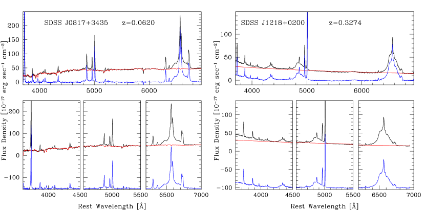
Figure 1: Stellar continuum subtraction. The original spectra are in black, the continuum templates are in red, and the residual emission lines are given in blue. The spectra shown are the observed flux densities, redshifted to $z=0$, vs. the the rest frame wavelength. The spectrum on the left is dominated by the galaxy continuum, while the one on the right is fit by a simple power law. The lower panels give close-ups of the [O II]$\lambda$3727, H$\beta$ and H$\alpha$ emission line regions; note that here the residual emission lines are displaced by $-150$(left) and $-100$(right) units for clarity.

The initial sample consists of 5511 objects with $z<0.5$, observed by SDSS as of June 2002 and classified as AGN by the spectroscopic pipeline. A subsample of 3216 AGN (hereafter the “parent” sample) with signal-to-noise ratio per pixel in the red continuum of $S/N\geq 7$, full coverage over the H$\alpha$ line region (rest frame 6000–6900 Å, an effective $z<0.332$ cut), and no spectral defects was selected. Before analyzing the H$\alpha$ line complex we subtract a sum of power law and galaxy continuum from each spectrum. The galaxy templates used in the subtraction were created by PCA of a few hundred high signal-to-noise ratio pure absorption line galaxy spectra observed by the SDSS (Hao et al., 2003). Each galaxy template covers the range 3814–7014 Å in the galaxy rest frame and consists of the eight largest galaxy eigen-spectra (in addition to the power law continuum and the possibility of including an A star spectrum to accommodate AGN and galaxies with dominant young stellar populations), with coefficients fit to best reproduce the continuum. The PCA method of generating stellar subtraction templates has the advantage of offering a unique solution with the use of only a handful of eigen-spectra (i.e. the orthogonality of the eigen-spectra guarantees uniqueness). Example continuum subtractions of selected double-peaked objects with dominant stellar (left panel) or power law (right panel) continua are shown in Figure 1. The power law fit is weighted toward the H$\alpha$ and H$\beta$ line regions ($\lambda_{rest}>4400$Å, excluding 150 Å around H$\alpha$ and H$\beta$ and 10 Å around the strong forbidden lines) whenever a single power law is insufficient to give a good overall fit, as shown in the right panel of Figure 1. The continuum subtracted spectra are binned to 210 km s^-1 pixel^-1 to smooth over any small scale features that might influence the broad line profile fits.

With 766 of the 3216 AGN visually selected to have symmetric as well as an unusually large fraction of asymmetric broad line profiles, we create line-profile eigen-spectra via PCA. The eigen-spectra cover the 6000–6900 Å rest frame region and use the continuum and stellar subtracted spectra. The advantage of using eigen-spectra at this step lies in the fact that a small number of these orthogonal “principal components” can represent the full variance in a sample with no loss of information. We exclude the narrow line regions from consideration when creating the eigen-spectra and flux-normalize all lines to $10^{-16}$ erg s^-1 cm^-2, fixing the 6130–6240 Å continuum to zero. Using the eigen-spectra we find the corresponding coefficients for all 3216 AGN that give good representations of the original line spectra (the largest 10–15 out of 168 possible coefficients are usually enough, but we use the first 20 to judge the goodness of the representation). Linear combinations of the first, second, forth and fifth coefficients ($c_{1}$, $c_{2}$, $c_{4}$, and $c_{5}$, see Figure 2 for the corresponding eigen-spectra) are then used to select 645 unusually asymmetric or broad AGN lines out of the original 3216. The coefficient selection combination, optimal for selection of an initial visual sample selected by eye by three of the authors (IVS, NLZ, and MAS) and presented in Strateva et al. (2003), is as follows:

$$0.64c_{1}+c_{2}<-0.084\quad\wedge\quad 0.55c_{2}+c_{4}<0.005\quad\wedge\quad 1.5c_{2}+c_{5}<-0.0045$$ (1)

At the second selection step, the 645 unusual AGN lines are fit with a sum of Gaussians: narrow H$\alpha$ $\lambda$6563 Å, [N II]$\lambda\lambda$6548, 6583 Å (constrained to 1:3 height ratio and the same width), [O I]$\lambda\lambda$6300, 6364 Å, and [S II]$\lambda\lambda$6716, 6731 Å, as well as two to four Gaussians for the asymmetric broad component of H$\alpha$. Most AGN line-profiles require more than two broad Gaussians for a good fit to the broad H$\alpha$ component, as can be seen in the four example fits of selected double-peaked objects shown in Figure 3. The broad component attributed to disk-emission is shown with a solid line above the spectrum in each case, and consists of three broad Gaussians in panels a), c), and d) (given separately with dashed lines) and two broad Gaussians in case b). A broad central H$\alpha$ component (defined as a component within 5 Å of the narrow H$\alpha$ line which is broader than it) is subtracted together with the narrow lines in panes b) and d), since this emission is likely to arise in a separate region, as is the case for the prototype disk-emitter Arp 102B (Halpern et al., 1996). Using the sum of broad Gaussians (less a central broad H$\alpha$ in some cases) we estimate whether the profile is single or double peaked (see Section 3.2 for more details). Because of the large number of parameters (three per Gaussian), we restarted the Levenberg-Marquardt fitting procedure (Press et al., 1999) with 10 different initial sets of parameters, taking as our final result the one with best $\chi^{2}$. Whenever two of the fits are similar in a $\chi^{2}$ sense, but the peak finding method finds two peaks in one case and only one in the other, the candidate is not considered a double-peaked AGN, with the exception of 10 interesting cases that are retained in an auxiliary sample as detailed in Appendix A. The sum of broad components of the fit (excluding any broad central component) is later used in Section 3.2 for measuring a number of line-characterizing quantities for comparison with models.

Table 1 lists all 85 disk-emitting candidates selected in the two-step procedure, arranged in order of increasing RA. Additional 31 objects of interest that were not identified by one of the steps of the algorithm but have interesting line profiles suggestive of disk emission are presented in Appendix A and listed separately in Table 2. The first column in both tables lists the official SDSS name in the format “SDSS Jhhmmss.s$\pm$ddmmss.s”, J2000; we will shorten this to “SDSS Jhhmm$\pm$ddmm” for identification beyond these tables. The second column gives the redshift, measured at the [O III]$\lambda$5007 line as appropriate for the AGN host; in all line profile discussions below we use velocity coordinates with respect to the narrow H$\alpha$ line. Columns three through seven in Tables 1 and 2 give the apparent model magnitude of the active galaxy in the SDSS ugriz passband system (corrected for Galactic extinction, following Schlegel, Finkbeiner & Davis, 1998) and the last column contains selection comments. The objects in Table 2 (hereafter the “auxiliary” sample) will be considered as an extra sample treated separately from the uniformly selected sample of 85 objects (hereafter “main” sample) of Table 1 in all subsequent discussions in this paper. The 85 objects of Table 1 are classified into five groups: prominent red shoulder objects (“RS”), prominent blue shoulder objects (“BS”), two prominent peaks (“2P”), blended peaks (“2B”), or complex many-broad Gaussian line (“MG”). A “+C” indicates that a central broad H$\alpha$ component is included in the fit. Figure 4 shows example line profiles for each of the first four types. In addition a comment “RL” marks the radio-loud AGN (see Section 4.3) in both Tables 1 and 2.

Twenty-two AGN were observed repeatedly, some multiple times. One of the reasons for repeat spectroscopic observations was to achieve acceptable signal-to-noise ratio on early plates, hence not all the data are of good quality. Nonetheless, we have 30 repeat observations of 22 of the candidate disk-emitting AGN with separations ranging from 3 days to 2 years. The repeat exposures are indicated as “repeat$N$,$P_{\textrm{\scriptsize{min}}}$-$P_{\textrm{\scriptsize{max}}}$” in Tables 1 and 2, where $N$ is the number of repeat observations, excluding the principal one, and $P_{\textrm{\scriptsize{min}}}$ and $P_{\textrm{\scriptsize{max}}}$ are the minimum and maximum separations, in days (for $N=1$ the format reduces to“repeat1,$P$”).

Disk-emission candidates are selected based on their characteristic double-peaked H$\alpha$ line profiles. H$\beta$ line profile selection could, in principle, permit extension of the sample to higher redshifts, but isolating the broad H$\beta$ component is difficult. One reason is that the region around H$\beta$ is sometimes heavily contaminated by Fe emission while in other cases the broad line component is very weak or completely absent from the spectra (i.e. in objects with a large Balmer decrement), even when H$\alpha$ is clearly double-peaked. Selection based on the shape of Mg II $\lambda$2800 is similarly ambiguous since Mg II sits on a pedestal of Fe emission; moreover narrow self-absorption at the systemic redshift is often present, making it even harder to use Mg II for identification of disk-emitters. Nonetheless we have three interesting objects which were found by chance based solely on their Mg II and H$\beta$ profiles (see Figure 5).

3.2 Gaussian Fits and Line Profile Measurements

In order to compare statistically the observed line profiles with theoretical profiles, we measure a series of profile-characterizing quantities which are related to one or more of the model disk parameters as described in Section 5 below. The sum of broad Gaussians (excluding any central broad H$\alpha$ component) fitted to each candidate disk-emission AGN provides us with smooth representations of the observed profiles ideal for such measurements. Using these smooth profiles we measure the full width at half maximum (FWHM), the full width at quarter maximum (FWQM), their respective centroids FWHMc and FWQMc, the positions of the blue and red peaks ($\lambda_{\textrm{\scriptsize{red}}}$ and $\lambda_{\textrm{\scriptsize{blue}}}$), and the blue and red peak-heights ($H_{\textrm{\scriptsize{red}}}$ and $H_{\textrm{\scriptsize{blue}}}$). All positional measurements (FWHM, FWQM, FWHMc, FWQMc, $\lambda_{\textrm{\scriptsize{red}}}$, and $\lambda_{\textrm{\scriptsize{blue}}}$) are quoted in km s^-1 with respect to the narrow H$\alpha$ line position; the peak heights ($H_{\textrm{\scriptsize{red}}}$ and $H_{\textrm{\scriptsize{blue}}}$) are given in $10^{-17}$ erg s^-1 cm^-2 Å^-1. The peak positions are found by requiring a first derivative numerically close to zero and negative second derivative. If this criterion fails and the two peaks are not obvious in the sum of broad Gaussians (for example, for strongly one-shouldered objects), we use an inflection point in a few cases to stand for the second peak (see panel c of Figure 3 for an example). By relaxing the numerical threshold for the inflection point search at this step we can also estimate the peak positions for most cases of auxiliary sample AGN flagged as “NotGausSelect” in Table 2. The line widths at half and quarter of the maximum are measured by first finding the two points on each side of the profile numerically closest to the desired fraction of the maximum, and then linearly interpolating between them to find the precise position. Table 3 gives the H$\alpha$ measurements for both the main and auxiliary samples of disk-emission candidates, with separate measurements at each epoch for objects observed more than once (a total of 138 entries for the 116 objects).

We measure the line-characterizing quantities for each observed epoch separately instead of combining the profiles, for two reasons. For repeat observations over short time intervals ($<$6 months up to a year), no strong variation in the line shape is expected, and we can use these profiles separately to quantify the errors of the selection and line-parameter measurement algorithms. Whenever the interval between observations is on the order of years — the timescale for which substantial changes in the profile are expected (Gilbert et al., 1999) — combining the profiles will result in loss of information. Figure 6 gives example line profile fits to repeat observations of the same object over half a year. The variations in the line profile are not large, but are significant (see bottom right panel of Fig. 6), and result in substantial difference in the measured blue peak position.

Broad line variability in AGN can be caused by changes in the illuminating continuum (Gondhalekar, Horne, & Peterson, 1994), the dynamics of the emitting gas (Gilbert et al., 1999), or changes in the BLR structure. The timescales of interest to us are the light-crossing and dynamical timescales, since they are sufficiently short to produce visible profile change in our sample. Changes in the illuminating continuum (reverberation) which cause changes in the observed line flux, but not the line shape (Wanders & Peterson, 1996), are apparent on light-crossing timescales ($\tau$${}_{\textrm{\scriptsize{light}}}$$=R/c$), which are of order 6–60 days for a $10^{8}$–$10^{9}$M_⊙ black hole and a BLR size of $R=10^{3}R_{G}$ (where M_⊙ is the mass of the Sun and $R_{G}=GM/c^{2}$ is the gravitational radius around a black hole of mass $M$, $G$ is the gravitational constant and $c$ the speed of light). If the accretion disk is non-axisymmetric, the disk inhomogeneities will orbit on dynamical timescales — $\tau$${}_{\textrm{\scriptsize{dynamical}}}$ $\sim$ 6 $M\,R^{3/2}$ months — causing changes in the line shape.

3.3 Error Estimates

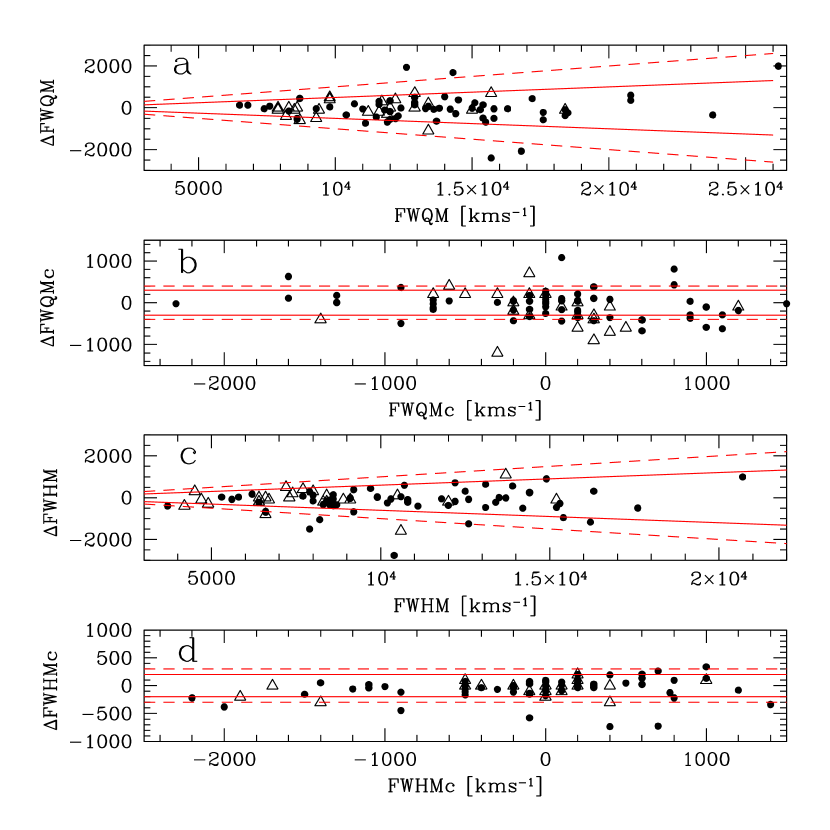
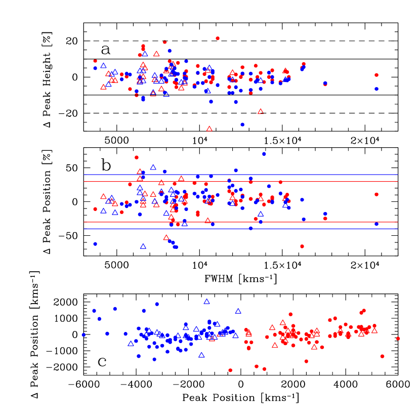
Figure 8: Error estimates for the measured line parameters from the reprocessed subsample (filled circles) and the repeat observations of the same AGN (triangles). 80% of the measured parameter variation of the combined subsamples is enclosed within the solid lines on each plot, 90% within the dashed lines. Top: a) $\Delta$ FWQM (in kms^-1) vs. FWQM, the solid and dashed lines correspond to 5% and 10% error, respectively. b) $\Delta$ FWQM centroid (in kms^-1) vs. FWQM centroid. c) $\Delta$ FWHM (in kms^-1) vs. FWHM, the solid and dashed lines correspond to 6% and 10% errors. d) $\Delta$ FWHM centroid (in kms^-1) vs. FWHM centroid. Bottom: a) Percent difference in measured heights for the red (red symbols) and blue (blue symbols) peaks vs. FWHM. b) Percent difference in measured peak positions vs. FWHM. c) Difference in peak positions vs. peak position.

Errors in the final line parameter measurements can occur in any of the processing steps — the continuum subtraction, the Gaussian fitting, or the line parameter estimation. Although the line measurements of the Gaussian fits are very precise, some complex line profiles allow alternative peak representations — for example in cases with only one prominent shoulder (see Fig. 7 for an extreme example). In order to estimate the fitting errors we compare the line parameter measurements obtained in an earlier separately processed subsample of 63 line profiles (hereafter “reprocessed” sample) with those of our final sample given in Table 3. We also compare the differences in line measurements between repeat observations over timescales of less than a year (24 cases), after normalizing the lines to a common total flux. The two methods give similar results, although they test for discrepancies coming from algorithm issues in the first case, and S/N ratio and repeatability in the second. The earlier processed subsample uses the unbinned original spectra for the Gaussian fits, has a slightly older version of the continuum subtraction algorithm and performs only one Gaussian fit, instead of restarting the fits with different initial values. The differences in line measurements found by both methods in each of the 2 subsamples (the reprocessed subsample and the repeatedly observed one) are given in Figure 8. We define the errors as the limits containing 80% of the combined subsamples’ variation; for example, the FWQM measurement differences are within 5% of the value measured in km s^-1 for 80% of the combined subsamples. The FWHM measurements (in km s^-1) have $\sim$6% error, the FWHM centroids about $\pm 200$ km s^-1, the FWQM centroids about $\pm 300$ km s^-1, the peak height errors are $\sim$10% of the flux density measured in units of $10^{-17}$ erg s^-1 cm^-2 Å^-1, the peak positions between 30% (red peaks) and 40% (blue peaks) of the measured position in km s^-1. The errors in all measured quantities are recorded in Table 4.

4 Double-peaked AGN Sample Properties

4.1 Emission Line Widths and Strengths

Eracleous & Halpern (1994), Eracleous (1998), and Ho et al. (2000) define a set of characteristics of the double-peaked disk-emitters which distinguish them from the majority of AGN. In their studies of predominantly lobe dominated, radio-loud AGN they find that, on average, the disk emitters have broad lines that are twice as broad as the typical radio galaxy or radio-loud AGN, have large contributions of starlight to their continuum emission, high equivalent widths of low-ionization forbidden lines like [O I]$\lambda$6300, and [S II]$\lambda\lambda$6716, 6731 (about twice that of average AGN), and line ratios, [O I]$\lambda$6300/[O III]$\lambda$5007 and [O II]$\lambda$3727/[O III]$\lambda$5007, that are systematically higher. With the exception of the stellar contribution to the continuum, we investigate these properties for the main and auxiliary samples in relation to those of the parent sample of 3216 AGN with $z<0.332$. Due to the aperture bias resulting from the $3^{\prime\prime}$ SDSS fibers, the relative stellar contribution we measure would be biased toward higher values for higher redshift objects, and consequently we postpone the estimate of stellar contribution to the continuum until small aperture data is available.

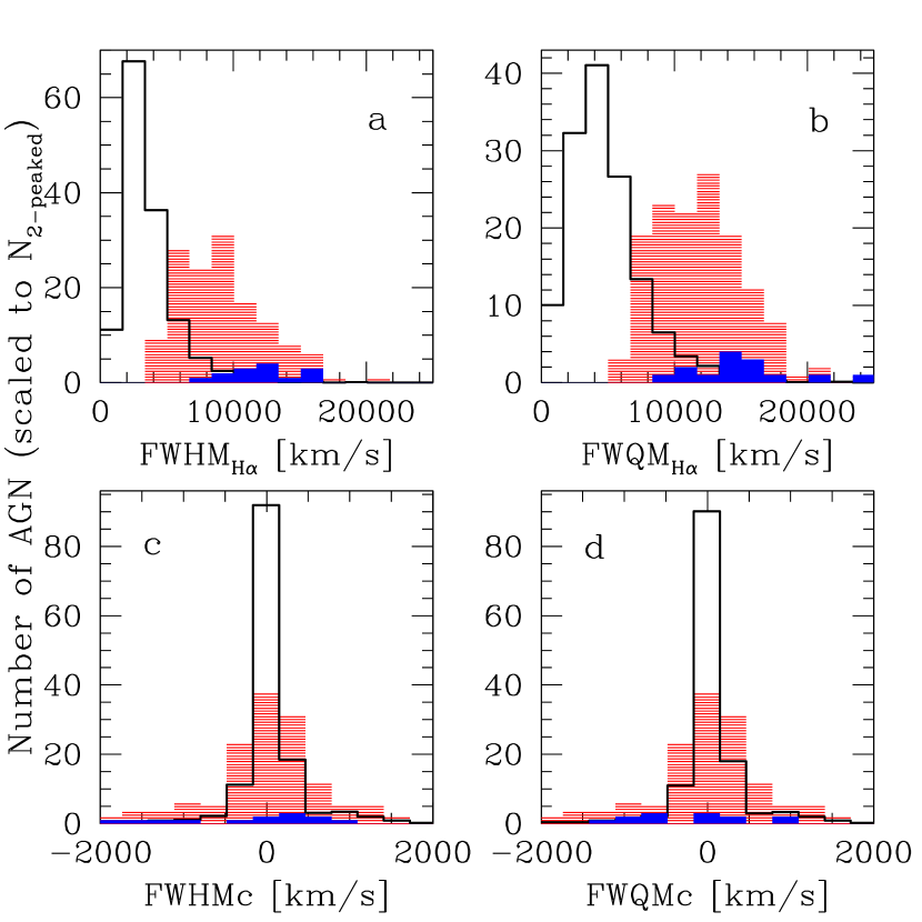
Figure 9: Comparison between the distributions of the FWHM (panel a), FWQM (b), FWHM centroid (c), and FWQM centroid (d) of the parent $z<0.332$ AGN sample (black hollow histograms) and the selected double-peaked emitters from Table 3. The solid blue histogram shows the distribution of radio loud double-peaked AGN. The total number of AGN have been scaled to the number of double-peaked AGN, except for the subsample of radio-loud AGN.

Figure 9 shows the comparison between the selected double-peaked (red shaded histogram) and parent (black hollow histogram) AGN samples’ FWHM, FWQM and their respective centroids. The PCA step of the double-peaked AGN selection procedure preferentially picks up broader than usual H$\alpha$ lines, selecting about 56% of all objects with FWQM$>$6000 km s^-1 (those broad lines are in turn about one-third of all 3216 AGN lines considered). The final Gaussian-fit selected disk-emission candidates (shown with red histogram in Figure 9) have even larger widths, with 90% of the main and auxiliary samples having FWQM$>$8000 km s^-1; there are only five objects with FWHM$<$5000 km s^-1. Thus the PCA selection step is not restrictive, and we find than the disk-emission candidates have broader line profiles than the majority of AGN, in agreement with Eracleous & Halpern (1994). The radio loud subsample, which is better matched in properties to the sample of known disk-emission AGN, (14 out of our 17 radio loud AGN have Gaussian fit measurements for H$\alpha$, see Appendix A) has larger FWHM and FWQM than both the double-peaked and the parent samples of AGN.

The two lower panels in Figure 9 give the FWHM and FWQM line centroids for the double-peaked (red shaded histogram) and the parent sample of AGN (black hollow histograms). The two distributions are significantly different, with the double-peaked AGN having larger red (and blue!) shifts than the general AGN population. The larger redshifts of the double-peaked AGN are expected, as they arise naturally from gravitational redshift of the disk emission in the vicinity of the SBH. The large blueshifts cannot be explained by a simple axisymmetric disk emission, but could arise in a non-axisymmetric disk, as we argue in Section 6. The solid blue histogram shows 14 out of the 17 radio loud double-peaked AGN with H$\alpha$ centroid measurements. There is no significant difference in the distribution of the centroids for the radio loud double-peaked AGN in comparison with the full AGN sample.

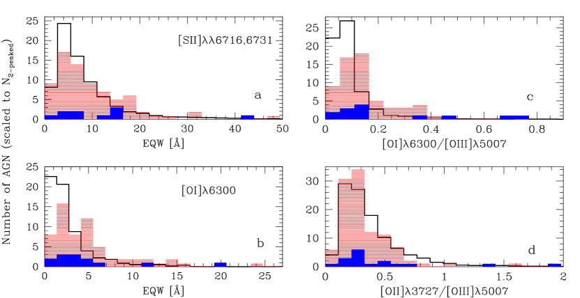
Figure 10: Comparison of the equivalent widths (panels a and b) and low-ionization line ratios (c and d) between the parent sample of AGN with $z<0.332$ (black histograms) and the selected double-peaked AGN (red shading). Note that the two samples are well matched in luminosity and redshift. The solid blue histogram shows the radio loud subsample from the sample of selected double-peaked AGN. The total number of AGN have been scaled to the number of double-peaked AGN, except for the subsample of radio-loud AGN. The double-peaked AGN tend to have large equivalent widths of [O I] and higher [O I]/[O III] flux ratios.

Because the stellar contribution to the continuum changes with redshift and we measure the line equivalent widths with respect to the total continuum (stellar + AGN power law, as in Eracleous & Halpern, 1994), the equivalent width measurements could depend on redshift. We measure the [O I]$\lambda$6300 and [S II]$\lambda\lambda$6716, 6731 equivalent widths with respect to the blue and red continuum in the immediate vicinity ($\sim$10Å on each side) of the lines. No trend of equivalent width with redshift is apparent. The distributions of the equivalent widths for the parent sample of 3216 AGN and the double-peaked AGN (of both main and auxiliary samples) are presented in Figure 10.

Overall, a large fraction of the double-peaked sample has low-ionization line equivalent widths and ratios similar to those of the parent sample. The double-peaked AGN tend to have larger equivalent widths of [O I]$\lambda$6300 and higher [O I]$\lambda$6300/[O III]$\lambda$5007 flux ratios than do the majority of AGN. A Kolmogorov-Smirnov (KS) test confirms that there is a significant difference between the distributions of the [O I]$\lambda$6300 equivalent widths and the [O I]$\lambda$6300/[O III]$\lambda$5007 flux ratios for the double-peaked and parent AGN samples (the null hypothesis, that the two distributions are the same is rejected with p-values of less than 0.1%). There is no strong evidence from Figure 10 or a KS test that the [S II]$\lambda\lambda$6716, 6731 equivalent widths and [O II]$\lambda$3727/[O III]$\lambda$5007 flux ratios of the double-peaked AGN are different from those of the majority of AGN. The sample of double-peaked AGN of Eracleous & Halpern (1994) is quite small (11 objects fitted with circular disk model) and the spread of measured equivalent widths is larger than that for their parent sample of 84 radio-loud AGN, which shifts the average of their disk-emission sample to larger equivalent widths. The radio loud part of our double-peaked sample is shaded blue in the histograms of Figure 10. There is no significant difference between the equivalent widths and line ratios of the radio-loud double-peaked AGN in comparison with the full double-peaked sample (nor is there a trend with the radio-loudness indicator of any of these quantities), but the number of radio loud objects (ranging from 10 objects with non-zero [S II]$\lambda\lambda$6716, 6731 equivalent width measurements to 17 objects with [O II]$\lambda$3727/[O III]$\lambda$5007 flux ratio measurements) is too small to state this with confidence.

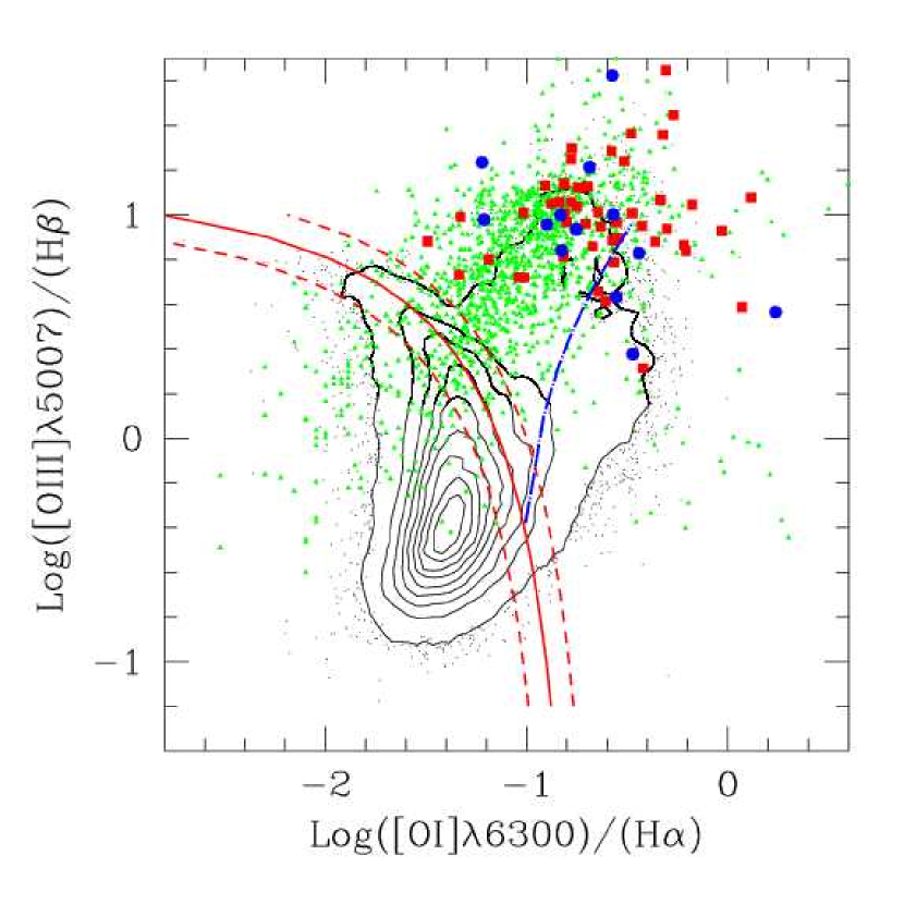
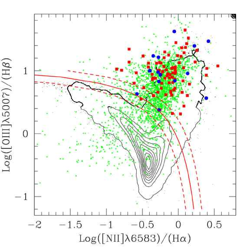
Figure 11: Position of double-peaked AGN (red squares) and the parent $z<0.332$ AGN sample (green triangles) on narrow line Veilleux-Osterbrock diagnostic diagrams. The radio loud AGN from the double-peaked sample are shown as solid blue circles. The black contours represent over 50,000 Sy2 and star-forming galaxies from the r$<17.77$ SDSS main sample (Hao et al., 2003). The solid red curve (the dashed curves correspond to the model uncertainty) is a theoretical prediction by Kewley et al. (2001): Sy2s occupy the portion of each graph above the red curve, normal star-forming galaxies below. The blue dot-dashed curve in the [O I]/H$\alpha$ vs. [O III]/H$\beta$ plot is Kewley’s theoretical prediction separating the LINERs (to the right of the line) from the Sy2s.

Figure 11 shows two of the Veilleux & Osterbrock (1987) AGN diagnostic diagrams. The theoretical results of Kewley et al. (2001), given as red solid lines, separate the Seyfert 2 active galaxies (Sy2s, lying above the solid red curves in both panels) from the majority of star-forming galaxies. The contours represent $\sim$50,000 galaxies from the main SDSS sample (with an apparent magnitude cut of r$<$17.77, Strauss et al., 2002) from Hao et al. (2003), showing the good agreement between the theoretically computed separation and the data. The parent sample of more luminous, higher redshift AGN used for this paper (green triangles) and the sample of double-peaked AGN (red squares) have similar narrow [O I]/H$\alpha$, [N II]/H$\alpha$, and [O III]/H$\beta$ flux ratios, with the [O I]/H$\alpha$ and [N II]/H$\alpha$ line-flux ratios 0.2 to 0.3 dex smaller than the lower luminosity Sy2s. The errors in our higher redshift sample narrow-line fluxes introduced by the subtraction of the broad line component can reach 20-40%. There is no difference between the narrow line ratios of the radio quiet (blue squares in Fig. 11) and radio loud (solid blue circles in Fig. 11) double-peaked AGN.

The dot-dashed blue curve in the [O I]/H$\alpha$ vs. [O III]/H$\beta$ plot in Fig. 11 is the Kewley et al. (2001) theoretical prediction separating the Sy2s, situated above and to the left of the curve, from the low-ionization nuclear emission region (LINER) galaxies to the right and below the curve. LINERs are believed to be low-luminosity AGN with normal narrow line regions which either have abnormally low ionization parameters or are powered by a combination of starburst and AGN. There is some evidence that LINERs are associated with disk emission, since double-peaked Balmer line profiles have appeared in well known LINERs NGC 1097, Pictor A and M81 (Storchi-Bergmann, Baldwin, & Wilson, 1993; Sulentic, Pietsch, & Arp, 1995; Halpern & Eracleous, 1994; Bower, Wilson, Heckman, & Richstone, 1996). Using Kewley’s criterion (situated below and to the right of the blue curve in Fig. 11) we find that 12 of the double-peaked AGN at low redshift are LINERs ($\sim$12% of the main and auxiliary samples). Uncertainties in the line ratios of 20-40% (0.1-0.2 dex) or in the theoretical curve ($\sim$0.1 dex, Kewley et al., 2001) could result in an under- or over-estimate of the fraction of LINERs ($\sim$9% of all selected AGN are within 0.1-0.2 dex of the separation line).

4.2 Colors and Host Galaxies

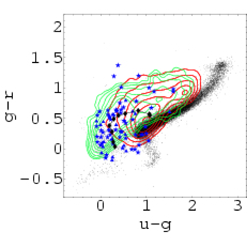
Figure 12: AGN host colors (blue stars for the main sample, blue triangles for the auxiliary AGN) compared to stellar colors (black dots), galaxy colors (red contours) with the characteristic morphological separation into early and late types, and the colors of the full AGN sample with $z<0.33$ (green contours). The black diamonds (upper right to lower left) are the average colors of AGN with redshifts between 0.025 and 0.475 in 0.05 redshift intervals.

The SDSS star-galaxy separation criterion requires that the PSF magnitude be fainter than the model magnitude by $>0.145$ for extended objects. The criterion is found to be $>$95% accurate for objects as bright as our sample (Abazajian et al., 2003). According to this criterion, 32% of our full sample (both main and the auxiliary sample) are spatially unresolved. About 44% of the candidates are sufficiently extended to attempt a crude visual classification; 60% of these appear to have early type morphologies (E, SO, Sa). Figure 12 gives the total galaxy+AGN colors for the main and auxiliary samples in comparison to the colors of stars, galaxies and all AGN with $z<0.33$. Since the colors of low redshift AGN are quite varied depending on the host galaxy and the strength of the central nuclear source, the u-g colors of low redshift sources could be significantly different from the average colors of either AGN or non-active galaxies.

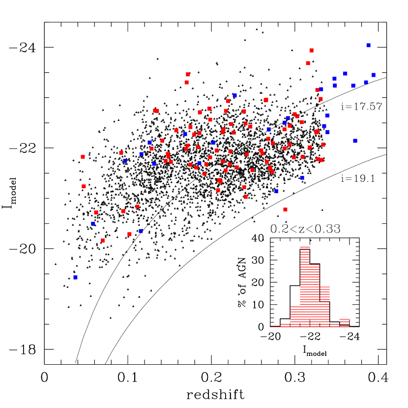
Figure 13: Absolute $i$-band magnitude distribution of double-peaked AGN from the main (red squares) and the auxiliary samples (blue squares) in comparison with that of the original sample of all $z<0.332$ AGN (small black symbols). The two curves denote the apparent magnitude limits for the AGN (lower curve, $i=19.1$) and the galaxy (upper curve, $i\approx$17.57) SDSS target selection for spectroscopy. The inset shows the absolute magnitude histogram for the $0.2<z<0.33$ subsamples of the main and original samples.

Table 5 lists the total (AGN+host galaxy) luminosities of our sources in erg s^-1 in the five SDSS bands, computed using $\Omega_{\lambda}=0.73$, $\Omega_{\textrm{\scriptsize{m}}}=0.27$, flat cosmology, with H${}_{\textrm{\scriptsize{o}}}$=72 km s^-1 Mpc^-1. The majority of the candidate disk-emitters have luminosities of a few $\times 10^{44}$ erg s^-1, similar to the average luminosity of all AGN observed with the SDSS in the $z<0.332$ redshift range. Figure 13 presents the redshift vs. absolute magnitude diagram. The majority of double-peaked candidates (shown in red for the main sample) have absolute magnitudes within a magnitude of I${}_{\textrm{\scriptsize{model}}}=-22$, similar to the rest of the AGN with $z>0.2$. This is equal to the faintest magnitude of the standard SDSS definition of a quasars, even though the model magnitudes used here overestimate the nuclear luminosity by up to a magnitude for nearby AGN by including the host galaxy contribution. From Figure 13 it appears that lower redshift ($z\lesssim 0.2$) double-peaked AGN tend to be more luminous than the average AGN, but the numbers are too small to make a statistically rigorous statement; moreover there are selection effects that affect the result, since about 1/3 of the AGN at $z<0.2$ were targeted for spectroscopy as “main galaxies” with a brighter apparent magnitude cut of $r<17.77$ (which corresponds to $i\lesssim 17.57$) while for $z>0.2$ almost all AGN are targeted by the AGN algorithm with a fainter cut at $i<19.1$.

4.3 FIRST counterparts

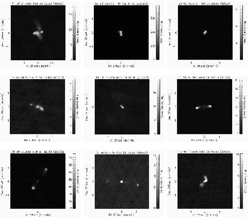
Figure 14: Nine of the ten radio matches of double-peaked AGN with prominent lobes. Note the peculiar radio morphology of SDSS J1130+0058 (top left, reminiscent of jet-reorientation) and the bow-like shape of SDSS J1346+6220 (bottom right).

The radio properties of disk-emission AGN described in the literature place the majority of them in the radio-loud category, consistent with the notion that disk-emission AGN are predominantly found in low-accretion rate, large black hole mass, massive bulge, radio-loud elliptical hosts (Eracleous & Halpern, 1994; Ho et al., 2000). In fact, 16 of the 116 AGN in the main and auxiliary samples of disk-emitters were targeted as FIRST sources (10/16 are also targeted as ROSAT sources, see below), with all 16 also making the AGN target cut based on colors. Since not all FIRST data were available at the time of SDSS object targeting, we repeated the SDSS-FIRST match for the 102 of the 116 double-peaked AGN which currently fall in the area of overlap of the two surveys. 31 sources out of these 102 have 20 cm FIRST counterparts within $2^{\prime\prime}$ of the SDSS position. The $2^{\prime\prime}$ search radius finds only core dominated sources and is smaller than the distance at which the number of random SDSS-FIRST associations starts becoming significant ($2^{\prime\prime}.5$, Ivezić et al., 2002, hereafter I02). Visual inspection of $4^{\prime}$$\times$$4^{\prime}$ images from FIRST revealed 4 additional lobe dominated sources. There are a total of 10 lobe (see Fig. 14) and 25 core dominated sources among the 35 FIRST detected objects. Two of the extended radio sources have peculiar morphologies: SDSS J1130+0058 (top left in Fig. 14) is reminiscent of X-shaped jet sources like 3C223.1 or 3C403, while SDSS J1346+6220 (bottom right in Fig. 14) has a bent radio jet.

The main sample of 85 candidate disk-emitters match FIRST sources within $60^{\prime\prime}$ (meant to include the lobe dominated sources as well, at the expense of increased match-by-chance contamination) in $\sim$30% of the cases, compared to $\sim$19% for the parent sample of 3216 AGN from which the selection of double-peaked profiles was made. Limiting ourselves to the core dominated sources only (matched within a $2^{\prime\prime}$ radius), $\sim$22% of the disk-emission candidates are FIRST sources, compared to $\sim$13% for the general sample of AGN in the same redshift range. In either case, candidate disk-emitters are $\sim$1.6 times more likely to be radio sources than the average AGN in the same redshift range. This difference is significant at the $3\sigma$ level. The ratio of lobe to core dominated sources is about 2:5 for both the double-peaked and the parent AGN sample.

Table 5 lists the integrated 20 cm luminosities for the 35 matched objects, using the sum of integrated flux densities to compute the luminosity in the cases of lobe dominated objects. Following I02, we define the ratio of radio to optical flux density, $R_{i}$ as:

$$R_{i}=\log(F_{\textrm{\scriptsize{20\,cm}}}/F_{i})=0.4(i-t)$$ (2)

where i is the i band SDSS PSF magnitude and $t$ is the 20 cm AB radio magnitude (Oke & Gunn, 1983) computed as $t=-2.5\log{(F_{\textrm{\scriptsize{20\,cm}}}/3631\textrm{Jy})}$ with $F_{\textrm{\scriptsize{20\,cm}}}$ the sum of integrated flux densities. Using the criterion $R_{i}>1$ for radio-loudness, we find that 17 of the 35 objects with FIRST matches are radio loud, 10 of which are in the auxiliary sample. The remaining 67 objects that are in the area covered by FIRST but not detected, must have radio flux densities of less than the FIRST detection limit of 1 mJy and thus $t>16.4$. Since all but 6 of them are brighter than $i=18.9$ in the optical, these additional 65 disk-emission candidates will have $R_{i}<0.4(18.9-16.4)=1.0$ and will be radio-quiet. By using the PSF magnitudes here we minimize the host galaxy contamination, so we do not expect this to have a large effect on the radio-loudness estimation. According to this estimate $\sim$68% of the disk emission candidates are radio-quiet. At most 37 of all disk-emission candidates (32%) could be radio loud, even if all objects not found in the area covered by FIRST (14 objects) and all undetected faint SDSS objects (6 objects with $i>18.9$) end up being radio-loud. This is in stark contrast to the fact that almost all previously known double-peaked AGN are radio-loud, as they were selected from radio loud samples (Eracleous & Halpern, 1994). If we repeat the statistics using only the main sample, we find 7 out of the 85 are detected in FIRST and radio-loud (8.2%), 65$/$85 are radio-quiet (76.5%), and 13$/$85 (15.3%) are too faint optically and not detected in FIRST or not in FIRST coverage.

The last column of Table 5 lists the optical to radio spectral indices, with the optical flux K-corrected to that at 2500 Å (see eqn. 4 below). Five of our disk-emission candidates also match sources from the Westerbork Northern Sky Survey (WENSS, Rengelink et al., 1997) within 60^′′. The WENSS is a long wavelength ($\lambda\lambda 85,92$ cm) radio survey of the sky north of $\delta=30^{\circ}$ to a limiting flux density of $\sim$18 mJy. Three of the FIRST-WENSS matched sources have radio lobes (SDSS J0806+4841, SDSS J1638+4335, and SDSS J1238+5325) in the FIRST images and for two of those (SDSS J0806+4841 and SDSS J1638+4335) the lobe emission dominates the radio emission, resulting in different 20 cm to 92 cm slopes of $\alpha_{20}^{92}=-0.2$ and $\alpha_{20}^{92}=-1.1$, respectively, compared to $\alpha_{20}^{92}=-0.5$ for the three core dominated sources. We use the spectra index of the core dominated sources (more appropriate for the majority of AGN), $\alpha_{20}^{92}=-0.5$, assuming $F_{\nu}\propto\nu^{\alpha}$, to K-correct the FIRST flux densities of all our sources to 20 cm. The optical to radio spectral index is then computed as follows:

$$\alpha_{\textrm{\scriptsize{or}}}=\left.-\log\left[{F_{\nu}(20\,\textrm{cm})\over F_{\nu}(2500\,\textrm{\AA})}\right]\right/\log{\left[\frac{2500\,\textrm{\AA}}{20\,\textrm{cm}}\right]}=0.1694\log{\left[\frac{F_{\nu}(20\,\textrm{cm})}{F_{\nu}(2500\,\textrm{\AA})}\right]}$$ (3)

The distribution of $\alpha_{\textrm{\scriptsize{or}}}$ indices is presented in the top panel of Figure 15.

4.4 ROSAT counterparts

For the general properties of a large sample of SDSS AGN matched with ROSAT all-sky survey (RASS) catalogs we refer the reader to Anderson et al. (2003). In the case of our disk-emission sample, 45 of the 116 AGN in the main and auxiliary samples were targeted as ROSAT (Voges et al., 1999, 2000) source counterparts for optical spectroscopy (all but 5 of them were also targeted as AGN or galaxies based on their optical photometry). We matched the 116 AGN from both the main and auxiliary samples against the bright (18811 objects, search radius $30^{\prime\prime}$, false detection rate 0.6%) and faint source (105924 objects, search radius $60^{\prime\prime}$, false detection rate 2.5%) ROSAT all-sky catalogs and found 47 ROSAT sources. Thus $\sim$41% of all AGN in our extended sample are detected in soft X-rays, $\sim$38% for the main sample and 48% for the auxilary sample. For comparison, the parent sample of 3216 AGN ($z<0.332$) have ROSAT matches in 28% of the cases. The candidate disk emitters from the main sample are thus 1.3 times more likely to have ROSAT counterparts. This is at most $2\sigma$ significant, considering that Poisson uncertainty alone contributes 15% to the error. The higher fraction of detections in the auxiliary sample is mainly due to its higher average redshift and the corresponding selection of more high-luminosity AGN. We used webPIMMs to convert from count rate in the 0.1–2 keV band to flux densities using HI column densities from the Leiden-Dwingeloo 21 cm maps (Hartmann & Burton, 1997) to estimate the unobscured flux assuming a power law continuum, $P(E)=E^{-\Gamma}$, with photon index $\Gamma=2$. For the bright source catalog matches we verified that the hardness ratios are consistent with a photon index of $\sim$2; the faint source hardness ratios are too noisy for this purpose. The unobscured 0.1–2 keV luminosities, which are again relatively low compared to luminous AGN (a few $\times 10^{44}$ erg s^-1 vs. $>10^{46}$ erg s^-1), are given in Table 5.

Using the u-g color, the u band (3543 Å) flux, and the redshift $z$, we can estimate the flux density at 2500 Å:

$$F_{\nu}(2500\,\textrm{\AA})=3631\times 10^{-0.4u-3.097\log[{1.417(1+z)}](u-g)}\>\textrm{Jy}$$ (4)

It is customary to define the optical to X-ray $\alpha_{\textrm{\scriptsize{ox}}}$ spectral index as:

$$\alpha_{\textrm{\scriptsize{ox}}}=\left.-\log\left[{F_{\nu}(2\,\textrm{keV})\over F_{\nu}(2500\,\textrm{\AA})}\right]\right/\log{\left[\frac{2500\,\textrm{\AA}}{2\,\textrm{keV}}\right]}=-0.3838\log{\left[\frac{F_{\nu}(2\,\textrm{keV})}{F_{\nu}(2500\,\textrm{\AA})}\right]}$$ (5)

with the unobscured $F_{\nu}(2\,\textrm{keV})$ approximated by:

$$F_{\nu}(2\,\textrm{keV})\approx\frac{\Delta F}{\Delta\nu}=\frac{F(1.9-2\,\textrm{keV})\,\textrm{erg\,s}^{-1}\textrm{cm}^{-2}}{0.1\,\textrm{keV}\times 4.836\times 10^{17}\textrm{Hz\,keV}^{-1}}\times 10^{23}\>\textrm{Jy}/(\textrm{erg\,s}^{-1}\textrm{Hz}^{-1}\textrm{cm}^{-2})$$ (6)

The optical to X-ray $\alpha_{\textrm{\scriptsize{ox}}}$ spectral indices are given in the ninth column of Table 5 and a histogram of the $\alpha_{\textrm{\scriptsize{ox}}}$ distribution is presented in the bottom panel of Fig. 15. Note that the auxiliary sample tends to have larger spectral indices, but the majority of disk-emission candidates have the canonical value of $\alpha_{\textrm{\scriptsize{ox}}}=1.4$, indistinguishable from that found by Anderson et al. (2003) for the general sample of ROSAT-SDSS matched AGN.

This concludes our discussion of the observed properties of the double-peaked AGN sample. We now proceed to compare the H$\alpha$ line profiles to those of model accretion disks.

5 Accretion Disk Models

In this section we summarize the theoretical accretion disk models used to simulate model emission line profiles. In the following section we will use these to create a series of model lines, spanning a range of disk parameters, for comparison with observations.

5.1 Axisymmetric (Circular) Disk

Prescriptions for computing model line profiles for circular accretion disks were taken from Chen & Halpern (1989). In brief, the models are based on a simple relativistic Keplerian disk which is geometrically thin and optically thick. Doppler boosting results in a higher blue peak than red and a net redshift of the whole line is observed. In order to reproduce the smoothness of the observed line profiles, either a continuous emissivity law or local turbulent broadening is added to the models; in what follows we use the local turbulent broadening models. The specific intensity of the disk is:

$$I_{\nu_{e}}(\xi,\nu_{e})=\frac{\epsilon_{0}}{4\pi}\frac{\xi^{-q}}{\sqrt{2\pi}\sigma}e^{\frac{(\nu_{e}-\nu_{0})^{2}}{2\sigma^{2}}}=\frac{\epsilon_{0}}{4\pi}\frac{\xi^{-q}}{\sqrt{2\pi}\sigma}\exp\left[-\frac{(1+X-D)^{2}\nu_{0}^{2}}{2\sigma^{2}D^{2}}\right]$$ (7)

for $\xi_{1}<\xi<\xi_{2}$, where $\xi\equiv r/R_{G}=rc^{2}/GM$ is the dimensionless distance from the black hole in units in which the gravitational constant and the speed of light are $G=c=1$, and $M$ is the black hole mass and $R_{G}$ is the gravitational radius. In eqn. 7, $\nu_{e}$ is the emitted frequency, $\nu_{0}$ is the rest frequency, $\nu$ is the observed frequency and $X\equiv\nu/\nu_{0}-1$. The slope of the surface emissivity power law ($\epsilon_{0}\>\xi^{-q}$) is $q$, while $\sigma/\nu_{0}$ is the dimensionless quantity characterizing the local turbulent broadening. The Doppler factor in the weak field approximation is given by:

$$D=\sqrt{1-3/\xi}(1+\xi^{-1/2}\>\sin{i}\>\sin{\phi})^{-1}$$ (8)

where $i$ is the disk inclination ($90^{\circ}$ is edge-on, $0^{\circ}$ is face-on), and $\phi$ is the azimuthal angle defined on the disk. Using the Lorentz invariance of $I_{\nu_{e}}/\nu_{e}^{3}=I_{\nu}/\nu^{3}$, we obtain an expression for the flux in the observer’s frame:

$$F=\int\!\!\!\int\!\!\!\int I_{\nu_{e}}(\nu/\nu_{e})^{3}\>d\nu\>d\Omega=\int F_{X}\>dX$$ (9)

where $d\Omega$ is the solid angle subtended by the disk as seen by the observer. If we denote the luminosity distance to the AGN as $d$, the line profile becomes:

$$F_{X}=\frac{\epsilon M^{2}\nu_{0}\cos{i}}{d^{2}}\int_{\xi_{1}}^{\xi_{2}}\int_{-\pi/2}^{\pi/2}\xi\>I_{\nu_{e}}\>D^{3}\>g(D\>)d\phi\>d\xi$$ (10)

where

$$g(D)=1+\xi^{-1}\left[\frac{2D^{2}}{D^{2}\cos{i}^{2}+\xi[D-\sqrt{1-3/\xi}]^{2}}-1\right]$$ (11)

and the term of order $\xi^{-1}$ is the light bending correction. To obtain the observed spectrum in units of erg cm^-2 s^-1 Hz^-1, one has to multiply F_X from eqn. 10 above by $G^{2}/(\nu_{0}c^{4})$.

Computing a circular disk line profile amounts to performing the double integration numerically in eqn. 10 after specifying five parameters: the inner and outer radii of the emitting ring, $\xi_{1}$ and $\xi_{2}$, the disk inclination, $i$, the slope of the surface emissivity power law, $q$, and the turbulent broadening $\sigma$. In theory, if these parameters were independent, they would correspond to the five parameters of a two-Gaussian fit representation of the double-peaked profile, resulting in a model that is fully constrained by the data. While the line shape determines the five model parameters given above, the overall normalization of the fit defines the product of emissivity and black hole mass – $\epsilon_{0}M^{2}$ – and this cannot lead to absolute black hole mass or emissivity estimates since the models set the size of the emitting ring only in relative units (i.e., in gravitational radii).

5.2 Elliptical Disk Model

If the red peak is stronger than the blue, or the profile is observed to be variable with successive blue and red dominant peaks (Gilbert et al., 1999), the circular disk emission model fails and some asymmetry in the disk must be invoked to reproduce the line asymmetry. Common choices are elliptical disks (thought to arise when a single star is disrupted in the vicinity of a black hole), warped disks (theorized to exist around rotating black holes; Bachev, 1999; Hartnoll & Blackman, 2000), spiral disks (Chakrabarti & Wiita, 1994; Hartnoll & Blackman, 2002; Karas, Martocchia, & Subr, 2001) or disks with a hot spot (Zheng, Veilleux, & Grandi, 1991). Without extensive data on profile variability, these models, which require many more free parameters (the elliptical disk model adds two more parameters, the hot spot and the warped disk models four extra parameters each), are often unjustified. In order to compare our observed kinematic profiles to both axisymmetric and non-axisymmetric disk models, we choose elliptical disk models to represent all non-axisymmetric disks. This choice is justified only by the relative simplicity of the computation, the addition of only two more parameters and our inability to distinguish between the various non-axisymmetric models with the current “snapshot” data.

In the case of an elliptical disk, the modified line profile equations derived by Eracleous et al. (1995) are reproduced below. Two extra parameters are added: the ellipticity, $e$, and the disk orientation, $\phi_{0}$. The orientation angle is measured with respect to the observer’s line of sight, $\phi_{0}=0^{\circ}$ when the apocenter points to the observer. The trajectory of particles in the disk is now elliptical, so the distance from the black hole varies:

$$\xi(\phi)=\frac{\tilde{\xi}\>(1+e)}{1-e\>\cos{(\phi-\phi_{0})}}$$ (12)

The line profile can again be calculated by integrating eqn. 10, except $g(D)$ is replaced by $\Psi(\xi,\phi)$:

$$\Psi(\xi,\phi)=1+\xi^{-1}\left(\frac{1-\sin{i}\cos{\phi}}{1+\sin{i}\cos{\phi}}\right)$$ (13)

The Doppler factor, $D$, in the elliptical disk case is:

$$\frac{1}{D}=\gamma\left\{\left(1-\frac{2}{\xi}\right)^{-1/2}-\\ \frac{e\>\sin{(\phi-\phi_{0})}\>\sqrt{1-(b/r)^{2}(1-2/\xi)}}{\sqrt{\xi(1-2/\xi)^{3}\>(1-e\>\cos{(\phi-\phi_{0})})}}+\frac{\sin{i}\>\sin{\phi}\>(b/r)\>\sqrt{1-e\>\cos{(\phi-\phi_{0})}}}{\sqrt{\xi(1-2/\xi)(1-\sin^{2}{i}\cos^{2}{\phi})}}\right\}$$

where $(b/r)$ is the impact parameter in the weak field approximation:

$$\frac{b}{r}\approx\sqrt{1-\sin^{2}{i}\>\cos^{2}{\phi}}\left[1+\frac{1}{\xi}\left(\frac{1-\sin{i}\cos{\phi}}{1+\sin{i}\cos{\phi}}\right)\right]$$ (14)

and $\gamma$ is the Lorentz factor:

$$\gamma=\left\{1-\frac{e^{2}\>\sin{(\phi-\phi_{0})}+(1-2/\xi)[1-e\>\cos{(\phi-\phi_{0})}]^{2}}{\xi\>(1-2/\xi)^{2}[1-e\>\cos{(\phi-\phi_{0})}]}\right\}^{-1/2}$$ (15)

5.3 Grid of Disk Model Line Profiles

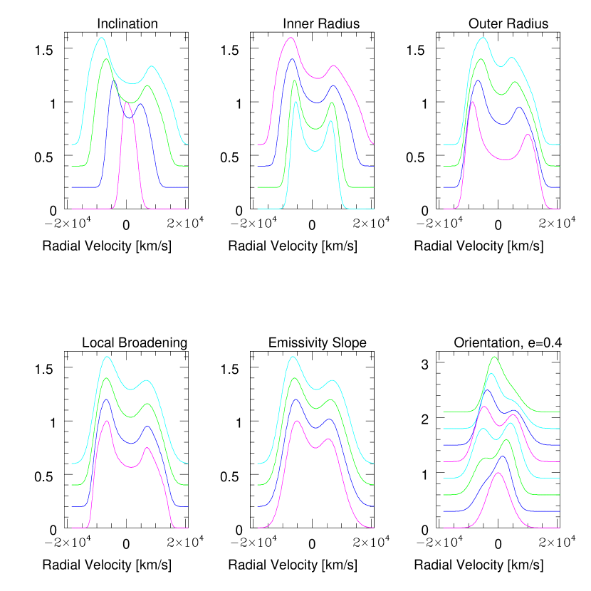
Figure 16: Clockwise, from top left: Variation of the line profile with inclination $i$, inner radius $\xi_{1}$, outer radius $\xi_{2}$, local broadening $\sigma$, emissivity slope $q$, and elliptical disk orientation, $\phi_{0}$ ($e=0.4$). All lines shown are circular disk models, except the lower right panel. In each case the varying parameter increases in value from the magenta to the cyan curve, taking all the values listed in Table 6. The values of the remaining non-varying parameters in the order ($i$,$\xi_{1}$,$\xi_{2}$,$\sigma$,$q$,$\phi_{0}$,$e$) are (from top left): ($...,3,300,1500,1200,0,0$), ($50,3,...,1500,1200,0,0$), ($50,3,300,...,1200,0,0$), ($50,3,300,1500,...,0,0$), ($50,...,300,1500,2400,0,0$), ($50,1.5,600,2500,2400,0.4,...$).

In order to understand the shapes of the line profiles and their parameter dependence we created a grid of 24,000 elliptical disk models (including the circular disk case for zero ellipticity), with all possible combinations of the parameters listed in Table 6. The parameter ranges were chosen to cover the range of known disk parameter estimates (Eracleous & Halpern, 1994). Example model line profiles are shown in Figure 16.

The effects of the disk model parameters on the computed line profiles are as follows. Changing the disk inclination, $i$, has the most dramatic effect on the line profile (see top left panel of Fig. 16). Low inclination angles result in narrow observed lines, which are frequently single peaked for $i<10^{\circ}$. The inner radius of the emitting ring, $\xi_{1}$, is smaller for broader line profiles and the Doppler boosting of the blue relative to the red peak is more pronounced for small $\xi_{1}$. The separation of the peaks is primarily a function of the outer emitting disk radius, $\xi_{2}$. As the outer radius increases, the inclusion of slower moving material effectively “fills in” the gap between the peaks (top right panel of Fig. 16), resulting in mostly single peak profiles for radii of a few $\times 10^{4}R_{G}$. The turbulent broadening, $\sigma$, smooths the line profile, while slightly decreasing the blue to red peak height ratio (bottom left panel of Fig. 16). For radiation arising in local dissipation of gravitational energy in the disk, the surface emissivity slope is expected to be $q=3$ (similarly for a combination of direct radiation from an elevated bulge and light scattered by a disk wind, the slope was found to be in the range between 2.5 and 3, Mardaljevic, Raine, & Walsh, 1988), but Eracleous & Halpern (1994) find examples of different slopes in their fits to observed profiles, some as small as $q=1.7$. Decreasing the slope of the surface emissivity makes the line profiles narrower, the blue side of the lines less steep, and suppresses the blue peak height. For non-axisymmetric disks, changing the orientation angle has a dramatic effect on the observed line profile. The lower right panel of Figure 16 shows 8 different orientations for a disk with ellipticity $e=0.4$. The profile changes from single to double peaked and back, while the blue peak is not necessarily dominant in the double-peaked phase. Note that these effects will be present also for warped disks and disks with a hot spot, thus comparing elliptical disk models to observed profiles will allow us to look for disk asymmetries, whatever their nature.

6 Comparison of Observed and Disk Model Line Parameters

Using the model line profiles, simulated over the parameter grid of Table 6, we can estimate which accretion disk parameters are consistent with the observed line shapes in a statistical sense. We chose this statistical comparison to individual accretion disk fits for each disk-emission candidate because it’s relatively computationally inexpensive, does not constrain each AGN line-profile to a specific model and can reveal the ranges of accretion disk model parameters despite the degeneracies accompanying each profile computation.

We perform the same line profile measurements on the model disk profiles as on the observed H$\alpha$ lines: we measure the FWHM, FWQM, their respective centroids, the positions of the blue and red peaks and the blue-to-red peak-height ratios for all disk models that actually show double peaks (a total of 784 models with $e=0$, and 13194 elliptical models).

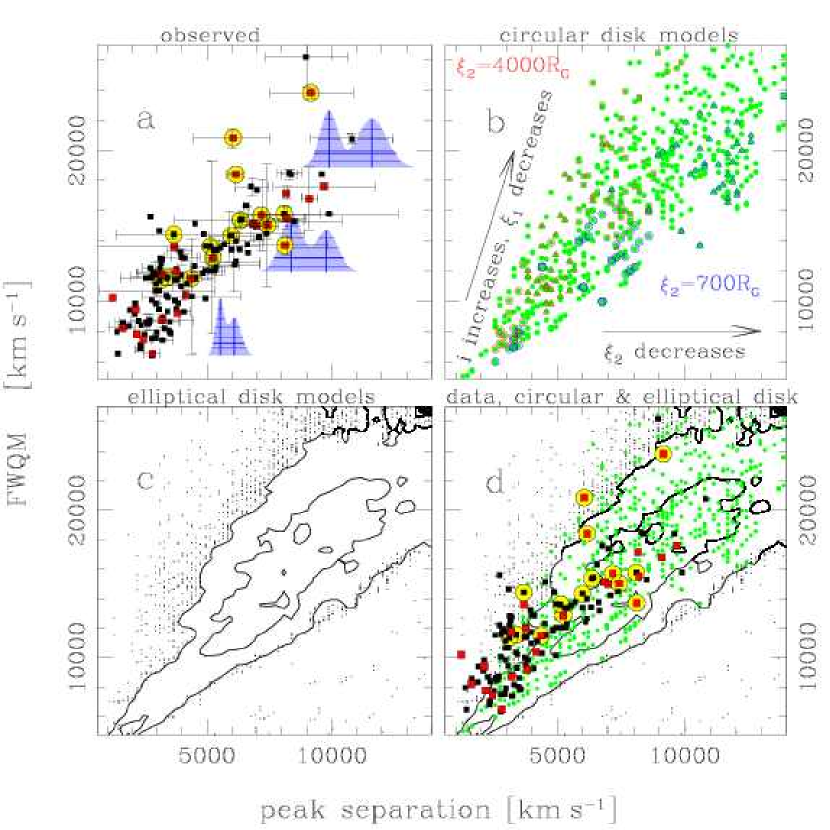
Figure 17: Comparison of observed and model line quantities. a) Observed peak separation vs. FWQM and 3 Gaussian fits for illustration. The filled black squares are the main sample from Table 1, the red squares are the auxiliary AGN from table 2, and the large yellow circles denote radio-loud AGN; errorbars are given for the 63 AGN with alternative processing. b) Circular disk models. Each point corresponds to a double peak model realization. The red (blue) symbols correspond to models with largest (smallest) outer radii. c) Non-axisymmetric (elliptical) disk models given as contours, the outliers as dots. d) Observed peak separation vs. FWQM compared to axisymmetric (green dots) and non-axisymmetric (black contours) disk models.

Figure 17 shows a comparison between observed and model disk lines for two of the line measurements. The observed peak separations vs. the FWQM for the main and auxiliary samples are given in panel a) with three example Gaussian fits for illustration. As noted above, the peak separation is a function of the outer radius, $\xi_{2}$, while the FWQM is determined by both the inclination and the inner radius of the emitting ring, $\xi_{1}$. The surface emissivity slope, $q$, also affects the line width, which increases for larger q values, but to a lesser extent. The top right panel gives the circular disk models. The small outer radius ($\xi_{2}=700R_{G}$) models are indicated in blue and the large outer radius ($\xi_{2}=4000R_{G}$) models in red. The elliptical disk models are presented in the lower left panel with contours, and the lower right panel shows the observed line parameters superimposed on both the elliptical and circular disk models. This comparison suggests that the data prefer large outer radii and disk inclinations smaller than 50^∘, with both axisymmetric and non-axisymmetric disk models agreeing with the data in this projection.

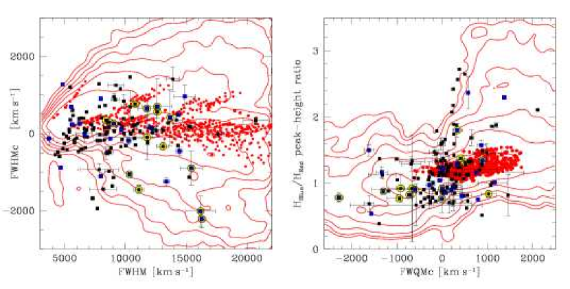
Figure 18: Observables suggest the need for non-axisymmetric disks. The observed values (black squares for the main sample, blue squares for the auxiliary sample, yellow circles around the radio-loud AGN) of the FWHM centroid (left) and the blue-to-red peak height ratio and FWQM centroid (right) are not all consistent with the circular disk models (red dots) in the sense that they can have FWHMc$<$0 and $H_{\textrm{\scriptsize{blue}}}/H_{\textrm{\scriptsize{red}}}<1$. The elliptical disk models (given as contours) are fully consistent with the data.

Figure 18 presents another comparison of observed to model line measurements, which suggests the need for non-axisymmetric disks to explain the observed values of the centroids at FWHM (left panel) and FWQM (right panel). The observed line measurements (black squares for the main sample, with errorbars from alternative processing, whenever available) have a much larger range of values than do the circular disk models (red dots), including negative centroids for the FWQM of order $-$1000 km s^-1 and stronger red peaks than blue $H_{\textrm{\scriptsize{blue}}}/H_{\textrm{\scriptsize{red}}}<1$ in the right panel of Figure 18) which are never realized for an axisymmetric disk. The elliptical disk models (given as contours), however, appear to be able to account for these line measurements. This is a non-trivial statement, since there are regions on the plot (e.g. the top and bottom left corners of the left panel or the top left half of the right panel) which both the models and the data avoid.

Using the seven line parameters (FWHM, FWQM, FWHMc, FWQMc, $\lambda_{\textrm{\scriptsize{red}}}$, $\lambda_{\textrm{\scriptsize{blue}}}$, H${}_{Blue}/$$H_{\textrm{\scriptsize{red}}}$) we compute the covariance matrix, $C$, for the observed line measurements in the main sample. For any set of seven model line measurements $\vec{x}$, we can compute the Gaussian equivalent probability that the model line is consistent with the observed values: $P(x)=\exp^{-1/2~{}\zeta^{2}}$, where $\zeta^{2}=(\vec{x}-\left<\vec{x}\right>)\cdot C^{-1}\cdot(\vec{x}-\left<\vec{x}\right>)$ is the squared deviation for this model from the observed values. Given the inverse of the covariance matrix (Table 7) and the average vector $\left<\vec{x}\right>=\{$$8852\textrm{\,km\,s}^{-1}$, $11702\textrm{\,km\,s}^{-1}$, $-2\textrm{\,km\,s}^{-1}$, $79\textrm{\,km\,s}^{-1}$, $2313\textrm{\,km\,s}^{-1}$, $-1939\textrm{\,km\,s}^{-1}$, $1.2\}$ we select the model disks whose measured line parameters are within $\zeta\leq 2$ of the observed values. This procedure allows us to obtain the input disk parameters (i.e. the inner and outer radii, the inclination, the surface emissivity slope, and the turbulent broadening) without performing detailed fits and constraining ourselves to a specific accretion disk model, while keeping in mind the degeneracy in the model parameters (e.g the inner radius, inclination and surface emissivity slope).

The total number of model lines with double-peaked profiles in the circular and elliptical disk cases are 784 and 13194, respectively, out of a total of 1200 circular and 23040 elliptical disk model lines. The $\zeta\leq 2$ criterion selects 99 out of 784 in the circular disk case and 444 out of 13194 in the elliptical case. Figure 19 presents histograms of the model parameters for the $\zeta\leq 2$ selected disks (shaded black) relative to the full number of double-peaked models (open histograms). The percent histograms in Figure 19 are computed with respect to the total number of double-peaked lines in both the circular and elliptical disk case. In other words, the open histograms sum to 100% while the shaded ones to 12.6% (99/784) in the circular and 3.4% (444/13194) in the elliptical disk case.

The initial set of disk models have equal numbers of models for each parameter value (that is equal number of models were run, for example, at each inclination). The fact that only 15% of the circular disk models shown as open histograms in Figure 19 have inclination of $i=20^{\circ}$ means that about 50% of the $i=20^{\circ}$ models are single peaked ($0.15\times 784$ out of $1200/5=240$ possible), compared to 90% single peaked $i=10^{\circ}$ models and 25% single peaked $i=30^{\circ}$ models for the circular disk case. On the other hand, the circular and elliptical disk models that were selected to have profiles within $\zeta\leq 2$ of the observed data, have inclinations $20^{\circ}<i<30^{\circ}$ in $\sim$90% of the cases. That is, the data strongly favor smaller inclination angles. This result is in good agreement with the result of Nandra et al. (1997), who argue that the Fe K$\alpha$ line profiles of 17 nearby ($z<0.05$) AGN are consistent with accretion disk emission from disks with an average inclination of $\left<i\right>=29^{\circ}\pm 3$, with all but two cases suggesting $i>50^{\circ}$. The lack of disks with very small inclinations ($i<10^{\circ}$) to our line of sight is a selection effect, but there is no a-priori reason why disks with high inclinations should be so rare. A possible explanation is that for inclinations in excess of $\hbox{$\sim$}50^{\circ}$ the obscuring torus, proposed to exist at larger distances from the central engine, prevents direct observation of the accretion disk, assuming that the small scale disk and large scale torus are coplanar. Whether they are coplanar is a matter of some debate in the literature (see the dust disk studies of Schmitt, Pringle, Clarke, & Kinney, 2002; de Koff et al., 2000). The inability of high inclination disk models to match our data argues that there is in fact substantial obscuration coplanar to the inner accretion disks of AGN. If larger-scale dust disks are not coplanar, perhaps the obscuration inferred from our data arises from the outer accretion disks in the form of a cool MHD disk wind (Königl & Kartje, 1994).

The inclination $i$, inner radius $\xi_{1}$, and surface emissivity slope $q$ are degenerate, in the sense that large $i$, small $\xi_{1}$ or large $q$ models give rise to line-profiles with large widths. As long as the surface emissivity slope (for a surface emissivity defined as $\epsilon_{0}\>\xi^{-q}$, $\xi_{1}<\xi<\xi_{2}$) is constrained to take values between 1.5 and 3 (see below), the seven measured quantities (FWHM, FWQM, FWHMc, FWQMc, $\lambda_{\textrm{\scriptsize{red}}}$, $\lambda_{\textrm{\scriptsize{blue}}}$, H_Blue, and H${}_{\textrm{\scriptsize{red}}}$) are sufficient to isolate the best model disk parameters consistent with the observations, despite the degeneracy. Due to relativistic effects in the strong gravity regime, emission from regions close to the black hole not only increases the line-profile width but also results in stronger line-asymmetries. For example, a small $\xi_{1}$ will increase the dominance of the blue peak together with the line width, while values of $q$ larger than 2 will tend to make the blue wing less steep.

The observed line profiles prefer model disks with flatter surface emissivity slopes ($1<q<2.5$, see bottom left panel of Fig. 19) than the $q=3$ predicted for local gravitational energy dissipation. In fact, if we allow $q$ to have even smaller values ($0.5<q<1.5$), than the values found for disk-emission AGN in the literature ($1.5<q<3$, Eracleous & Halpern, 1994), those would be selected as consistent with the observed line-profiles, forcing about a third of selected inclinations to values higher than $i=60^{\circ}$. In other words, the preference of the data for small inclinations is conditional on the surface emissivity having slopes steeper than $q\approx 2$. As mentioned in Section 5.3, all theoretical models of disk illumination that we are aware of predict surface emissivity decreasing with radius with a slope of about 3. Dumont & Collin-Souffrin (1990) have developed a self consistent model for Balmer line emission from geometrically thin, flaring Shakura-Sunyaev (1973) disks. They find that disks (heated only by viscosity) tend to be too cold at the radii corresponding to the Doppler shifts required by the observed line-widths and argue that an illuminating source is necessary to produce the Balmer line emission observed. The two disk illumination models considered plausible by the authors — a central point source and a diffuse medium that backscatters the central source radiation — both result in surface emissivity slopes of 2–3. Rokaki, Boisson, & Collin-Souffrin (1992) use the Dumont and Collin-Souffrin models to fit the Balmer line profiles together with the full spectral energy distributions of six Seyfert galaxies (two of which have double-peaked lines), and find that the diffuse medium illumination model agrees well with the data, with surface emissivity slopes between 2.1 and 3.6. In addition Nandra et al. (1997) find that the X-ray Fe K$\alpha$ line profiles of 17 nearby AGN are consistent with accretion disk emission from the innermost ($6R_{G}<\xi<1000R_{G}$) regions of the disk, with an average surface emissivity slope of $\left<q\right>=2.5\pm 0.4$, with all but one of the AGN preferring $q>1.5$ (see their Figure 6). Taking into account the above mentioned studies, we consider the high surface emissivity slope ($q>1.5$), low inclination ($i<50^{\circ}$) models more likely.

The models selected to be within $\zeta\leq 2$ of the observed line profiles in the main double-peaked sample tend to have larger outer radii (typically $\xi_{2}>2000R_{G}$, see middle right panel of Fig. 19), and local turbulent broadening of $780$ km s${}^{-1}<\sigma<1800$ km s^-1 (middle left panel of Fig. 19). There is a slight preference for ellipticities $e<0.4$ for non-axisymmetric models and no preference for the ellipse orientation (bottom right panel of Fig. 19).

To quantify the effects seen in Figure 18 (which imply the need for non-axisymmetric disk models) we compute the probability that each of the observed triplets of FWHMc, FWQMc and blue-to-red peak height ratio (H${}_{Blue}/$$H_{\textrm{\scriptsize{red}}}$) were drawn from the circular or the elliptical disk pools of values. We compute new $\zeta^{\prime}$-ellipsoids of both the circular and elliptical model triplets and calculate for each observed triplet the number of $\zeta^{\prime}$ away from these average models. In the circular disk case, using the main observed sample, we find that 62% of the observed triplets have $\zeta^{\prime}>3$ and are inconsistent the average axisymmetric model. In contrast all but one of the 112 observations ($>99\%$) are fully consistent with the elliptical models (i.e. the observed line measurements have $\zeta^{\prime}<3$).

7 Summary and Discussion

The present sample of double-peaked AGN, selected from the SDSS, is the largest set of such objects to date, with 85 disk-emission candidates in the main and an additional 31 candidates in an auxiliary sample. The main sample was selected uniformly from all AGN observed with SDSS with redshift $z<0.332$. The sample has H$\alpha$ lines which are broader than those of the general AGN population (FWHM$>5000$km s^-1), with larger red- and blueshifts of the broad H$\alpha$ component, in agreement with previous disk-emission sample statistics (Eracleous & Halpern, 1994). The selected AGN are 1.6 times more likely to be radio sources than the parent sample of $z<0.332$ AGN, but are predominantly (76%) radio quiet. This is substantially different from the existing sample of disk-emitters, which were mostly sought (and found) in radio-loud subsamples of AGN. The higher fraction of double-peaked AGN found in radio-loud samples ($\sim$10% for the radio-loud sample of Eracleous & Halpern, 1994, compared to $\sim$3% of all AGN with $z<0.332$ in this sample) is probably caused by the fact that both radio-loud quasars (as opposed to radio-loud galaxies, McCarthy, 1993) and double-peaked AGN tend to have very broad emission lines and are rare. If about 10% of all AGN are radio-loud and 10% of them are disk-emitters we expect to find double-peaked Balmer lines in only 1% AGN of the general broad-line AGN population. We find about 3%, the majority of them radio-quiet. Previous studies have thus overlooked a large part of the disk emission population consisting of radio-quiet AGN.

The selected double-peaked sample has medium luminosities, comparable to those of the average broad line AGN at the same redshift (a few $\times 10^{44}$erg s^-1). The equivalent widths of the low ionization lines also do not differ significantly from those of the majority of AGN, with the exception of [O I]$\lambda$6300 equivalent widths and [O I]/[O III] flux ratios, which tend to be larger for the double-peaked AGN. We find that $\sim$12% of the sample objects can be classified as LINERs according to Kewley’s selection criterion (Kewley et al., 2001).

Comparison with accretion disk emission models suggest that about 60% of the lines must originate in non-axisymmetric disks. This is similar to the fraction of double-peaked AGN that were not well fit by a circular disk model found by Eracleous & Halpern (1994). We need long term variability studies (the dynamical, thermal and sound-crossing times of typical accretion disks at $\sim$1000$R_{G}$ are of order half a year to 70 years for a 10⁸ M_⊙ black hole) to constrain well the various disk model asymmetries that give rise to line profile variation. A snapshot survey of the kind reported here cannot distinguish between various disk asymmetries; this justifies the use of one generic non-axisymmetric disk model (that of an elliptical disk) to detect disk asymmetries. The majority of radio-loud AGN are highly variable; similarly the known disk-emitters which have been followed up on timescales of decades (3C390.3, Arp 102B, etc.) were found to have line-profiles that varied significantly and required asymmetric disk models. Their identification with accretion disks have been strengthened, not diminished, by variability studies. For example, long term studies of double-peaked profile variations have imposed a lower limit of the combined mass of a black hole binary in excess of 10¹⁰ M_⊙, a result hard to reconcile with the observed ranges of black hole masses (Eracleous et al., 1997). Nonetheless, it is possible that double-peaked line profiles have more than one origin, and long term variability studies are essential to distinguish between the various models. In view of this we have initiated a follow-up variability study using Apache Point Observatory’s 3.5 m telescope. This should create, in time, a large sample with variability information which will be better suited to reject or confirm alternative models.

The binary black hole hypothesis for the double-peaked appearance of the H$\alpha$ lines is quite tempting, in view of the fact that galaxies merge and any black holes at their centers must pass through a binary stage. One of our objects (SDSS J1130+0058, top left in Figure 14) has a radio morphology similar to radio-jet reorientation objects like 3C52, 3C223.1, 3C403 and NGC 326. Radio-jet reorientation can be caused by mergers of supermassive black holes (Merritt & Ekers, 2002) or arise in the process of accretion disk realignment if the black hole and disk axes are initially misaligned (Dennett-Thorpe et al., 2002). In the case of a black hole merger, initially the interaction of the black hole binary with the bulge stars will make the orbit harder (i.e. shrink the orbit), but beyond about 1 pc, the mechanism responsible for bringing the binary down to the scale where gravitational radiation becomes important (10${}^{-2}-10^{-3}$ pc) is not clear (Merritt et al., 2003; Yu, 2002). Hence no solid theoretical predictions exist for the timescales associated with black hole mergers, in particular the sub-pc regions of interest here. Even if a theory predicting supermassive black hole coalescence existed, the fate of the gas feeding the activity adds more complexity. As Penston (1988) suggests, it is not obvious that the gas will stay close to each black hole, forming two separate BLRs, especially for unequal black hole mass mergers. It is plausible that the lower velocity gas will orbit the center of mass of the system, resulting in a single-peaked core, with two lower-intensity peaks emitted by the faster moving material blended with the core to reveal a single peaked profile (Chen, Halpern, & Filippenko, 1989).

An interesting parallel between accreting compact objects in our Galaxy (cataclysmic variables and low mass X-ray binaries) allows us to speculate on the long term changes in AGN accretion disks by analogy with the (much shorter timescale) evolution of the accretion disks around the white dwarf or black hole primary in these systems. Murray & Chiang (1997) propose a two zone line emission model for both AGN and compact accreting objects. In their model, the high ionization lines arise in the foot of the wind, just above the accretion disk (where the radial component of the velocity is small but large radial shear results in photons preferentially escaping from the back and front of the disk); this gas is optically thick and gives rise to single peaked lines. The low-ionization Balmer lines, on the other hand, could originate in the optically thin atmosphere of the disk and have double-peaked line profiles arising from disk rotation.

Dwarf novae, for example, are thought to be in a quiescent state, with low accretion rates. They show double peaked Balmer line profiles (clearly originating in the disk as proved by secondary eclipses) and have no high ionization lines. When they go into outburst, high ionization, single-peaked lines appear in the disk wind. Nova-like variables, in contrast, are almost constantly in outburst and very few show double-peaked Balmer lines. They have high ionization lines (e.g. He II) and the high ionization lines are single-peaked. Chiang and Murray’s idea is that in outburst state (always for nova-like variables, rarely for dwarf-novae), the accretion rate increases dramatically and the radiation becomes powerful enough to drive a wind. The high ionization (as well as the low ionization lines at times) originate in the base (or sometimes higher up) in the disk wind. In low, quiescent accretion states, the Balmer lines come from the disk and are double-peaked, and there are no high ionization lines coming from the disk.

Very few of the double-peaked AGN have been observed in the UV to date with sufficient signal-to-noise ratio to consider high-ionization line profiles (i.e. C III, C IV, Ly$\alpha$). The prototype disk-emitter, Arp 102B, has single peaked high-ionization lines narrower than the Balmer lines (Halpern et al., 1996). If this fact remains true for the majority of AGN with double-peaked Balmer lines, we could draw a direct parallel between the double-peaked AGN and quiescent dwarf-novae. Current findings classify double-peaked AGN as predominantly low-luminosity, low accretion rate systems relative to the majority of AGN (Eracleous & Halpern, 1994; Ho et al., 2000). The lack of big blue bump, combined with new theoretical models of low-rate accretion, suggests that the inner part of the disk is elevated into the quasi-spherical structures (the “ion torus” of Chen, Halpern, & Filippenko, 1989) of Advection Dominated Accretion Flow (ADAF) or Advection Dominated Inflow-Outflow (ADIOS) models (Igumenshchev, Abramowicz, & Narayan, 2000; Igumenshchev & Narayan, 2002; Ball, Narayan, & Quataert, 2001). Thus AGN with double-peaked Balmer lines could be viewed as the supermassive black hole analogs of dwarf-novae, in states of low accretion and luminosity, with the broad low-ionization emission originating in the parts of the disk just outside the elevated ion-torus, providing the excess energy and high-ionization lines arising in a weak wind. According to this view, the accretion rate and radiation pressure in the majority of AGN is substantially higher, resulting in a radiation driven (or MHD driven, see Proga, Kallman, Drew, & Hartley, 2002) wind and predominantly single peaked high and low ionization lines.

Acknowledgments

We are grateful to Michael Eracleous, Luis Ho, Jules Halpern, Bogdan Paczynski, and Wei Zheng for their advice and stimulating discussions; we also acknowledge the helpful comments of an anonymous referee. We wish to thank Doug Finkbeiner for his help with obtaining the HI column densities from the Leiden-Dwingeloo 21 cm maps. IVS and MAS acknowledge the support of NSF grant AST-0071091. IVS acknowledges the NASA Applied Information Systems Research Program (AIRSP) for partial support. Funding for the creation and distribution of the SDSS Archive has been provided by the Alfred P. Sloan Foundation, the Participating Institutions, the National Aeronautics and Space Administration, the National Science Foundation, the U.S. Department of Energy, the Japanese Monbukagakusho, and the Max Planck Society. The SDSS Web site is http://www.sdss.org/. The SDSS is managed by the Astrophysical Research Consortium (ARC) for the Participating Institutions. The Participating Institutions are The University of Chicago, Fermilab, the Institute for Advanced Study, the Japan Participation Group, The Johns Hopkins University, Los Alamos National Laboratory, the Max-Planck-Institute for Astronomy (MPIA), the Max-Planck-Institute for Astrophysics (MPA), New Mexico State University, University of Pittsburgh, Princeton University, the United States Naval Observatory, and the University of Washington.

Appendix A The Auxiliary Sample of Double-peaked AGN

Thirty-one objects of interest were not identified by one of the two steps of the selection algorithm but have line profiles suggestive of disk emission and are included in this auxiliary sample. The list of additional objects was presented in Table 2. The first column lists the object name in the format “SDSS Jhhmmss.s$\pm$ddmmss.s”, J2000, the second the redshift, columns three through seven give the apparent model magnitude corrected for Galactic extinction, and the last column contains selection comments.

The majority (21) of the 31 additional objects listed in Table 2 were missed on the PCA step, because their redshift was too high ($z>0.332$, 14 objects marked “HiZ”, including the three $z\approx 0.6$ objects with Mg II selection), because they were flagged as having spectral defects (two objects marked “badFlag”), because the automatic redshift estimate failed to recognize the H$\alpha$ line and assigned an incorrect high redshift (four objects marked “wrongZ”) or because they failed the eigen-spectra coefficient cut (one object marked “NotPCASel”). All but five of those 21 were fit with multiple Gaussians and selected by the double-peak finding step. The five AGN missed on the PCA step for which only part of the H$\alpha$ line is included in the spectral coverage (2/5) or H$\alpha$ is out of range (3/5) are flagged “NoParam” in Table 2.

The remaining ten auxiliary objects listed in Table 2 (marked “NotGausSel”) were missed during the Gaussian fit selection because the two peaks are blended and were missed by the inflection point selection (8/10) or because of a wrong set of initial parameters in a many-Gaussian fit (2/10). Eight of the ten were run through the peak finding algorithm with relaxed inflection point thresholds (the remaining 2 are flagged “NoParam” in Table 2).

Appendix B Vacuum Wavelengths

The wavelengths in SDSS spectra are given in vacuum, corrected to the heliocentric reference frame. Given a vacuum wavelength $\lambda_{vac}$ in Å, the conversion to air wavelength is given by (Morton, 1991):

$$\lambda_{air}=\frac{\lambda_{vac}}{(1.0+2.735182\times 10^{-4}+131.4182/\lambda_{vac}^{2}+2.76249\times 10^{8}/\lambda_{vac}^{4})}$$ (B1)

The conventional air wavelengths and the SDSS vacuum wavelengths for the lines commonly used in this paper are listed in Table 8.

Figure 2: The six largest eigen-spectra of the H$\alpha$ line region used in the PCA step of the double-peaked AGN selection. The vertical lines denote the positions of the narrow line regions which were excluded from consideration.

Figure 3: Example Gaussian fits. The original spectrum is binned to $\sim$210 km s^-1 pixels with the sum of Gaussians fit overlaid (thick line). The spectral error is shown below, displaced to a negative value (10% of each plot’s maximum flux density) for clarity. The sum of broad components attributed to disk emission are shown above with a solid line, while all broad components are given separately with dashed lines. The solid vertical lines from the top of each plot point to the positions of the two peaks. a) Three broad-component fit. b) Three broad-Gaussian fit, with a central broad H$\alpha$ component. c) Three broad-component fit, with the blue peak estimate given by the inflection point of the profile at $-2300$ km s^-1. d) Four broad-component fit with a red wing and a broad central H$\alpha$.

Figure 4: Examples of H$\alpha$ selected disk-emission candidates from each type: a) strong red shoulder (RS), b) strong blue shoulder (BS), c) two separate peaks (2P), and d) blended peaks (2B). The plot details are as in Figure 3.

Figure 5: Low ionization lines of three disk-emission candidates selected based on their Mg II and H$\beta$ (bottom right) line profiles. The spectra are smoothed to $\sim$500 km/s. Note the broad Fe emission blueward of H$\beta$ in the bottom right panel.

Figure 6: Example H$\alpha$ profile variation of a single object over 5 epochs, and corresponding line profile measurements. Successive observations (from top left down and from top right to the middle panel) show small variations in the line profiles on scales of 2-3 days to 219 days. Bottom right: The broad line profiles (displaced by 1 unit for clarity and scaled to the same line flux) for all 5 observations with the MJD indicated on the right. Note the large variations in the measured blue peak position.

Figure 7: Line-parameter variation due to alternative processing. The profile measurements of a line with an alternative fit (bottom panel) results in notably different red and blue peak positions and heights from these in the final analysis (top panel). The plot details are as in Figure 3, except the residuals replace the error spectra here and the line-profile measurements are listed in each case. The top panel fit is slightly better in a $\chi^{2}$ sense and is preferred.

Figure 15: Distribution of the optical-radio (top) and optical-X-ray (bottom) spectral indices for the FIRST and ROSAT detected AGN. The hollow histograms are for the main plus auxiliary sample, while the solid black histograms are for the auxiliary sample alone.

Figure 19: Model parameters for disk models whose line profile measurements are $\zeta<2$ away from the observed lines in the 7-dimensional space of FWHM, FWQM, FWHMc, FWQMc, $\lambda_{\textrm{\scriptsize{red}}}$, $\lambda_{\textrm{\scriptsize{blue}}}$, and $H_{\textrm{\scriptsize{blue}}}/H_{\textrm{\scriptsize{red}}}$ are given in black shaded histograms (which sum up to a total of 12.6% selected in the circular disk case and 3.4% in the elliptical), compared to the initial range of model parameters resulting in double peaked lines (open histograms, sum up to 100% for each of the circular and elliptical disk cases). Note that initially all model parameters were distributed equally in each direction, so a smaller percent of models within a particular open histogram bin means the rest were in single peaked lines.

Table 1: Double Peak H$\alpha$ AGN sample: Coordinates and Apparent Magnitudes

SDSS ID	Redshift	$u$	$g$	$r$	$i$	$z$	Comments
SDSS J000710.02+005329.0	0.3159	17.04	16.76	16.56	16.64	16.01	2P+C, repeat1,337
SDSS J000815.46$-$104620.5	0.1986	19.23	18.06	17.12	16.61	16.42	RS
SDSS J001224.03$-$102226.3	0.2200	17.07	17.03	16.83	16.49	16.62	RS
SDSS J004319.75+005115.3	0.3083	17.84	17.91	17.80	17.75	16.93	2P+C, repeat1,332
SDSS J005709.93+144610.3	0.1718	16.02	16.01	15.82	15.36	15.58	RS+C
SDSS J011140.03$-$095834.9	0.2064	19.08	18.56	17.77	17.32	17.04	2B
SDSS J013253.31$-$095239.5	0.2597	18.42	18.37	18.10	17.88	17.49	2P, repeat1,31
SDSS J013407.89$-$084129.9	0.0699	19.07	17.72	17.02	16.56	16.32	2B, repeat1,31
SDSS J014901.09$-$080838.1	0.2093	19.73	19.25	18.44	17.94	17.79	RS
SDSS J022014.57$-$072859.2	0.2136	18.22	18.24	17.63	17.04	16.98	MG
SDSS J023253.42$-$082832.1	0.2652	17.98	17.82	17.26	16.94	16.55	RS
SDSS J024052.82$-$004110.9	0.2466	18.59	18.14	17.50	17.28	17.15	2P+C, repeat1,378
SDSS J024703.24$-$071421.7	0.3340	19.89	19.60	18.76	18.40	17.55	RS+C, RL
SDSS J024840.04$-$010032.7	0.1840	19.44	18.38	17.49	16.97	16.64	2P
SDSS J025220.89+004331.3	0.1696	17.93	17.70	17.21	16.81	16.61	2B, repeat1,61
SDSS J025951.73$-$001522.7	0.1018	18.89	18.31	17.87	17.30	17.31	RS, repeat4,30,358
SDSS J034931.03$-$062621.0	0.2877	18.35	18.29	17.93	17.72	17.31	RS+C
SDSS J073927.24+404347.4	0.2081	19.58	18.96	18.48	18.13	18.07	2P
SDSS J074157.26+275519.9	0.3256	18.82	18.46	18.13	18.09	17.40	2B
SDSS J075930.77+352803.8	0.2886	20.54	20.31	19.62	19.32	18.88	RS+C
SDSS J080310.58+293233.8	0.3277	18.99	18.98	18.68	18.64	17.89	2P+C
SDSS J081329.29+483427.9	0.2738	18.05	18.04	17.87	17.87	17.38	2P, repeat1,27
SDSS J081700.40+343556.3	0.0620	18.95	17.36	16.42	15.73	15.56	2P+C, RL
SDSS J081916.30+481745.5	0.2228	18.53	18.60	18.05	17.52	17.38	RS, repeat1,27
SDSS J082113.71+350305.0	0.2936	18.82	18.52	18.17	18.07	17.73	BS
SDSS J082125.37+421908.5	0.2220	19.06	18.77	18.22	17.77	17.66	RS
SDSS J082133.61+470237.3	0.1283	18.93	17.56	16.67	16.14	15.94	RS, RL
SDSS J082205.25+455349.2	0.2998	18.11	18.02	17.64	17.52	17.08	2B
SDSS J082406.23+334244.9	0.3179	19.02	18.81	18.26	18.33	17.51	2P
SDSS J083225.35+370736.2	0.0920	15.91	15.96	16.05	15.45	15.73	MG+C
SDSS J083826.50+371906.7	0.2110	19.27	19.10	18.52	17.99	18.01	RS
SDSS J084110.88+022952.1	0.3322	18.88	18.96	18.76	18.69	18.03	BS
SDSS J084535.38+001619.5	0.2613	19.31	18.96	18.34	17.96	17.52	2P
SDSS J091459.05+012631.3	0.1977	18.28	17.63	16.80	16.38	16.17	2P+C, repeat1,26
SDSS J091828.60+513932.1	0.1855	17.63	17.34	17.07	16.71	16.72	2B
SDSS J092515.00+531711.8	0.1862	19.22	17.84	16.84	16.31	16.09	RS+C
SDSS J093509.47+481910.2	0.2237	18.16	17.79	17.42	16.99	17.27	MG
SDSS J093844.46+005715.8	0.1704	18.50	17.30	16.47	15.50	15.65	RS, repeat1,287
SDSS J100443.44+480156.5	0.1986	19.45	18.67	17.89	17.36	17.29	2P+C
SDSS J101405.89+000620.3	0.1412	19.38	17.79	16.81	16.21	15.95	2P
SDSS J103202.40+600834.5	0.2939	19.26	19.01	18.12	17.70	17.23	RS
SDSS J104108.19+562000.4	0.2304	19.70	19.32	18.27	17.92	17.83	2P+C
SDSS J104128.60+023205.0	0.1820	19.25	18.71	17.89	17.35	17.13	2P
SDSS J104132.78$-$005057.5	0.3029	18.11	18.00	17.71	17.59	16.98	MG+C
SDSS J110742.77+042134.2	0.3269	18.87	18.82	18.36	18.08	17.55	BS, repeat1,3
SDSS J112751.95+675042.8	0.1940	18.17	18.02	17.83	17.44	17.51	RS
SDSS J113021.00+022211.5	0.2410	17.48	17.54	17.48	17.16	17.20	BS+C
SDSS J113021.42+005823.0	0.1325	17.98	16.79	15.88	15.46	15.25	BS, RL
SDSS J113633.09+020747.5	0.2390	18.35	18.00	17.38	16.90	16.74	2B
SDSS J114335.36$-$002942.4	0.1715	18.01	17.82	17.30	16.77	16.83	BS+C, repeat2,76,375
SDSS J115047.48$-$031652.9	0.1486	18.98	17.81	17.06	16.64	16.34	2P
SDSS J115227.12+604817.5	0.2703	19.39	19.26	18.58	18.32	17.77	RS+C
SDSS J115644.11+614741.6	0.2265	17.88	17.80	17.60	17.19	17.16	RS+C
SDSS J121855.80+020002.2	0.3270	17.43	17.26	17.13	17.26	16.55	BS+C
SDSS J122009.55$-$013201.2	0.2879	18.57	18.58	18.28	18.10	17.56	2B
SDSS J130927.67+032251.8	0.2665	18.50	18.60	18.37	18.17	17.73	2B+C, repeat1,266
SDSS J132834.14$-$012917.6	0.1515	18.36	18.05	17.45	16.80	16.85	BS, RL
SDSS J133312.43+013023.7	0.2171	19.00	18.78	18.30	17.84	17.93	RS, RL
SDSS J135107.04+653127.4	0.2988	18.47	18.49	18.33	18.37	17.67	BS+C
SDSS J140019.28+631427.0	0.3309	18.24	17.96	17.57	17.47	17.10	2P
SDSS J140720.70+023553.1	0.3094	19.57	19.41	18.73	18.45	17.80	2P+C
SDSS J141454.55+013358.6	0.2704	19.52	19.53	18.71	18.35	17.81	BS
SDSS J141613.37+021907.8	0.1580	18.90	17.84	16.84	16.27	16.13	RS+C, RL
SDSS J141946.04+650353.0	0.1478	18.38	17.75	17.05	16.58	16.43	BS, repeat1,4
SDSS J142424.22+595300.6	0.1348	15.95	15.92	15.83	15.51	15.56	RS
SDSS J142754.77+635448.4	0.1453	18.36	17.86	17.18	16.68	16.48	2P
SDSS J143455.31+572345.3	0.1749	17.32	17.06	16.87	16.45	16.42	BS, repeat2,8,95
SDSS J154019.58$-$020505.4	0.3200	16.39	16.39	16.33	16.42	15.88	2P+C
SDSS J154534.55+573625.1	0.2681	19.17	18.75	18.00	17.73	17.29	2B
SDSS J160548.03$-$010913.0	0.2425	19.73	19.28	18.27	17.79	17.56	RS
SDSS J170102.29+340400.6	0.0945	18.56	18.05	17.59	16.67	16.90	BS+C, repeat1,7
SDSS J171806.84+593313.4	0.2728	18.74	18.89	18.61	18.43	17.96	2P
SDSS J172102.47+534447.2	0.1918	19.10	18.76	18.12	17.60	17.51	BS+C
SDSS J172711.83+632241.9	0.2175	17.12	17.04	16.93	16.66	16.74	2P, repeat1,95
SDSS J173038.27+550016.7	0.2491	19.25	18.98	18.54	18.17	17.91	2B, repeat4,3,219
SDSS J210109.57$-$054747.3	0.1794	18.23	17.91	17.15	16.66	16.41	2P
SDSS J211353.33$-$061241.2	0.2411	19.48	19.25	18.91	18.62	18.59	RS
SDSS J214555.04+121034.2	0.1113	18.52	18.01	17.46	16.96	16.81	2B
SDSS J214935.23+113842.1	0.2393	20.13	19.71	18.84	18.41	18.16	2P+C
SDSS J222913.62+000840.9	0.2657	19.07	18.32	17.34	16.93	16.51	2P
SDSS J223336.71$-$074337.1	0.1750	19.14	18.55	17.76	17.20	16.99	BS
SDSS J230443.47$-$084108.6	0.0471	15.69	15.27	15.08	14.59	14.52	BS
SDSS J231254.90$-$011620.6	0.2139	18.74	18.38	17.88	17.62	17.38	2P
SDSS J232721.96+152437.3	0.0460	16.22	15.11	14.44	13.95	13.64	BS+C
SDSS J233254.46+151305.4	0.2146	17.53	17.55	17.34	16.99	17.02	2P

Note. — The apparent magnitudes quoted here (Photo version 5.3) are total model galaxy magnitudes computed by convolving an exponential or de Vaucouleurs model with the PSF. The uncertainty in the magnitudes is at the few percent level, mostly due to photometric calibration, except in a few cases for u and z band measurements, where photon statistics dominate the error.

Table 2: Double Peak H$\alpha$ Auxiliary Sample: Coordinates and Apparent Magnitudes

SDSS ID	Redshift	$u$	$g$	$r$	$i$	$z$	Comments
SDSS J011734.84$-$011135.6	0.1855	19.23	18.68	17.89	17.31	17.33	NotGausSel
SDSS J021259.60$-$003029.6	0.3942	17.71	17.53	17.62	17.44	17.06	HiZ, NoParam
SDSS J021655.88$-$005228.9	0.2778	19.82	19.70	18.94	18.86	18.27	NotGausSel
SDSS J022930.92$-$000845.4	0.6091	20.11	19.66	19.51	19.00	18.94	HiZ, NoParam, Mg IISelect, RL
SDSS J030021.41$-$071458.9	0.3883	16.88	16.63	16.82	16.81	16.55	HiZ, NoParam
SDSS J032559.97+000800.8	0.3602	17.08	17.06	17.13	17.18	16.71	HiZ, repeat1,32
SDSS J075407.96+431610.6	0.3475	17.28	17.18	17.13	17.19	16.57	HiZ, RL
SDSS J080644.41+484149.2	0.3700	17.51	17.48	17.52	17.49	17.00	HiZ, repeat1,27, RL
SDSS J090436.96+553602.7	0.0372	16.89	16.55	16.16	15.87	15.68	MG NotGausSel, NoParam
SDSS J093653.85+533126.9	0.2281	17.29	17.06	16.86	16.47	16.60	NotGausSel
SDSS J100027.44+025951.3	0.3390	19.10	18.50	17.99	17.86	17.21	HiZ
SDSS J102738.54+605016.5	0.3314	17.75	17.51	17.36	17.28	16.92	wrongZ, RL
SDSS J114051.59+054631.1	0.1315	19.58	17.91	16.99	16.50	16.15	wrongZ
SDSS J121154.86+604426.1	0.6370	20.02	19.63	19.70	19.37	19.32	HiZ, NoParam, Mg IISelect, RL
SDSS J123807.77+532556.0	0.3478	17.26	17.30	17.30	17.33	16.69	HiZ, RL
SDSS J132442.44+052438.8	0.1154	18.81	18.58	18.36	17.53	17.82	wrongZ
SDSS J133338.30+041804.0	0.2022	18.52	18.26	17.70	17.11	17.10	wrongZ
SDSS J133433.25$-$013825.4	0.2917	18.30	18.28	17.74	17.53	16.99	NotGausSel, RL
SDSS J133957.99+613933.4	0.3723	19.04	18.79	18.63	18.60	17.92	HiZ
SDSS J134617.55+622045.5	0.1163	16.92	16.83	16.57	16.02	16.06	NotGausSel, NoParam, RL
SDSS J152139.66+033729.2	0.1261	16.94	16.91	16.74	15.98	16.31	badFlag
SDSS J163545.62+481615.0	0.3088	19.09	19.23	18.89	18.86	18.12	NotGausSel
SDSS J163856.54+433512.6	0.3391	18.44	18.39	18.22	18.19	17.44	HiZ, RL
SDSS J171049.88+652102.2	0.3853	17.72	17.69	17.62	17.53	17.15	HiZ
SDSS J205032.30$-$070131.2	0.1686	17.67	17.61	17.17	16.50	16.70	NotGausSel
SDSS J212501.21$-$081328.6	0.6246	17.39	16.83	16.87	16.78	16.85	HiZ, repeat1,22, NoParam, Mg IISelect
SDSS J215010.52$-$001000.7	0.3351	18.11	18.00	17.93	18.04	17.52	HiZ
SDSS J222132.40$-$010928.7	0.2878	18.87	18.56	17.91	17.59	17.15	badFlag
SDSS J223302.68$-$084349.1	0.0582	18.37	16.86	16.26	15.81	15.61	NotPCASel
SDSS J230545.66$-$003608.6	0.2687	19.52	18.95	18.01	17.55	17.13	NotGausSel, RL
SDSS J235128.76+155259.1	0.0966	17.55	16.85	16.24	15.72	15.63	NotGausSel

Table 3: H$\alpha$ profiles: Line Parameter Measurements

SDSS ID	MJD	Flux	FWHM	FWHMc	FWQM	FWQMc	$H_{\textrm{\scriptsize{red}}}$	$\lambda_{\textrm{\scriptsize{red}}}$	$H_{\textrm{\scriptsize{blue}}}$	$\lambda_{\textrm{\scriptsize{blue}}}$
SDSS J0007+0053	51456	7300	9800	400	12300	600	30.1	2300	33.9	$-$2200
SDSS J0007+0053	51793	5500	9500	300	11900	400	22.5	2600	27.9	$-$2200
SDSS J0008$-$1046	52141	1600	9600	1200	14700	0	6.7	2800	5.7	$-$300
SDSS J0012$-$1022	52141	13400	5500	1200	9500	2100	41.2	4600	87.0	800
SDSS J0043+0051	51462	1900	11900	100	15200	500	5.8	2000	7.4	$-$2600
SDSS J0043+0051	51794	4000	11800	$-$200	14200	$-$100	14.0	3600	18.8	$-$3400
SDSS J0057+1446	51821	36200	9900	800	13300	1100	144.7	2600	144.9	$-$1300
SDSS J0111$-$0958	52177	900	5400	100	7100	100	5.0	1400	6.7	$-$900
SDSS J0117$-$0111	52202	3700	5600	200	7800	0	21.6	1500	26.8	$-$700
SDSS J0132$-$0952	52147	3600	15300	200	18500	300	10.9	4600	10.7	$-$3700
SDSS J0132$-$0952	52178	3900	15200	200	18400	100	12.2	4800	11.4	$-$3500
SDSS J0134$-$0841	52147	1300	8300	200	11400	600	7.0	2000	5.7	$-$1800
SDSS J0134$-$0841	52178	1300	8400	0	11700	500	7.2	1900	5.8	$-$2000
SDSS J0149$-$0808	52174	1000	5400	0	7500	300	4.4	2200	8.4	$-$600
SDSS J0216$-$0052	52209	1700	9600	100	11800	300	6.6	2600	8.6	$-$600

Note. — This table is published in its entirety in the electronic edition of The Astrophysical Journal. A portion is shown here for guidance regarding its form and content. “MJD” in the second column refers to the last five digits of the Modified Julian Date. All positional measurements (FWHM, FWHMc, FWQM, FWQMc, the red peak position, $\lambda_{\textrm{\scriptsize{red}}}$, and the blue peak position, $\lambda_{\textrm{\scriptsize{blue}}}$) are in km s^-1 relative to the narrow H$\alpha$ line; the line flux is in $10^{-17}$ erg s^-1 cm^-2, the peak heights, H${}_{\textrm{\scriptsize{red}}}$ and H${}_{\textrm{\scriptsize{blue}}}$, are in $10^{-17}$ erg s^-1 cm^-2 Å^-1.

Table 4: Errors in Measured Line Quantities

Parameter	Error
FWHM	6%
FWHMc	200 km s-1
FWQM	5%
FWQMc	300 km s-1
$H_{\textrm{\scriptsize{red}}}$ and $H_{\textrm{\scriptsize{blue}}}$	10%
$\lambda_{\textrm{\scriptsize{red}}}$	30%
$\lambda_{\textrm{\scriptsize{blue}}}$	40%

Note. — Errors are estimated from repeat observations and processing as detailed in Section 3.3. Errors in FWHM, FWQM, FWHMc, FWQMc, $\lambda_{\textrm{\scriptsize{red}}}$ and $\lambda_{\textrm{\scriptsize{blue}}}$ are measured in km s^-1 or percent thereof; peak height errors are in percent of flux density in units of $10^{-17}$ erg s^-1 cm^-2 Å^-1.

Table 5: Optical, radio and X-ray luminosity and spectral indices

SDSS ID	L${}_{\textrm{\scriptsize{U}}}$	L${}_{\textrm{\scriptsize{G}}}$	L${}_{\textrm{\scriptsize{R}}}$	L${}_{\textrm{\scriptsize{I}}}$	L${}_{\textrm{\scriptsize{Z}}}$	L${}_{\textrm{\scriptsize{0.1-2\,keV}}}$	L${}_{\textrm{\scriptsize{20\,cm}}}$	$\alpha_{\textrm{\scriptsize{ox}}}$	$\alpha_{\textrm{\scriptsize{or}}}$
SDSS J0007+0053	14.62	14.06	12.94	9.82	14.65	5.27	$6.72\times 10^{-5}$	1.4	0.10
SDSS J0008$-$1046	0.67	1.47	2.67	3.50	3.48	$\cdots$	$\cdots$	$\cdots$	$\cdots$
SDSS J0012$-$1022	6.20	4.78	4.40	4.92	3.64	$\cdots$	$7.59\times 10^{-5}$	$\cdots$	0.14
SDSS J0043+0051	6.61	4.60	3.90	3.34	5.93	2.34	$7.06\times 10^{-5}$	1.5	0.11
SDSS J0057+1446	9.38	7.03	6.41	8.00	5.46	4.04	$\cdots$	1.5	$\cdots$
SDSS J0111$-$0958	0.84	1.01	1.60	1.98	2.14	$\cdots$	$\cdots$	$\cdots$	$\cdots$
SDSS J0117$-$0111	0.58	0.71	1.13	1.58	1.29	$\cdots$	$\cdots$	$\cdots$	$\cdots$
SDSS J0132$-$0952	2.61	2.03	1.99	1.99	2.38	$\cdots$	$\cdots$	$\cdots$	$\cdots$
SDSS J0134$-$0841	0.08	0.21	0.31	0.38	0.40	$\cdots$	$\cdots$	$\cdots$	$\cdots$
SDSS J0149$-$0808	0.48	0.55	0.89	1.16	1.11	0.69	$\cdots$	1.2	$\cdots$
SDSS J0212$-$0030	13.28	11.64	8.20	7.91	9.37	$\cdots$	$9.90\times 10^{-5}$	$\cdots$	0.12
SDSS J0216$-$0052	0.84	0.70	1.07	0.94	1.36	$\cdots$	$\cdots$	$\cdots$	$\cdots$
SDSS J0220$-$0728	2.01	1.47	1.97	2.77	2.44	0.77	$2.70\times 10^{-5}$	1.5	0.14
SDSS J0229$-$0008	4.16	4.68	4.11	5.38	4.74	$\cdots$	$4.33\times 10^{-3}$	$\cdots$	0.54
SDSS J0232$-$0828	4.10	3.53	4.53	4.97	5.94	$\cdots$	$\cdots$	$\cdots$	$\cdots$

Note. — This table is published in its entirety in the electronic edition of The Astrophysical Journal. A portion is shown here for guidance regarding its form and content. The luminosities are in units of $10^{44}$ erg s^-1 computed using $\Omega_{\lambda}=0.73$, $\Omega_{\textrm{\scriptsize{m}}}=0.27$, flat cosmology, with H${}_{\textrm{\scriptsize{o}}}$=72 km s^-1 Mpc^-1.

Table 6: Model Disks – Grid Parameters

Parameter	Value 1	Value 2	Value 3	Value 4	Value 5	Value 6	Value 7	Value 8
$i$ [∘]	10	30	50	70	20	…	…	…
$q$	$1.5$	$2.0$	$2.5$	$3.0$	…	…	…	…
$\xi_{1}$ [$R_{\textrm{\scriptsize{G}}}$]	$200$	$300$	$600$	$800$	…	…	…	…
$\xi_{2}$ [$R_{\textrm{\scriptsize{G}}}$]	$700$	$1500$	$2500$	$4000$	…	…	…	…
$\sigma$ [km s-1]	$780$	$1200$	$1800$	$2400$	…	…	…	…
$e$	$0$	$0.2$	$0.4$	$0.7$	…	…	…	…
$\phi_{0}$ [∘]	$0$	$45$	$90$	$140$	$180$	$230$	$280$	$320$

Note. — $i$ is the inclination, with $i=90^{\circ}$ disks viewed edge on. The surface emissivity is parameterized by $q$, as $\epsilon_{0}\>\xi^{-q}$. The inner and our radii, $\xi_{1}$ and $\xi_{2}$, are in units of the gravitational radius, $R_{\textrm{\scriptsize{G}}}$=GM/c². $\sigma$ is the local turbulent broadening, $e$ the ellipticity, and $\phi_{0}$ is the ellipse orientation, with $\phi_{0}=0^{\circ}$ equivalent to the apocenter pointing to the observer. $e=0$ refers to the circular disk models and the orientation angle $\phi_{0}$ is irrelevant. Also if $\xi_{1}=800$, then $\xi_{2}\neq 700$. This reduces the number of all possible arrangements of parameters from $4^{6}\times 8=32,768$ to $24,000$. The $i=20^{\circ}$ disk models were run only for circular disks ($\approx$ 960 additional models).

Table 7: Inverse of the Covariance Matrix for the Observed Line Measurements

	FWHM	FWQM	FWHMc	FWQMc	$\lambda_{\textrm{\scriptsize{red}}}$	$\lambda_{\textrm{\scriptsize{blue}}}$	H${}_{Blue}/$$H_{\textrm{\scriptsize{red}}}$
FWHM	$2.4056\times 10^{-6}$	$-1.6648\times 10^{-6}$	$5.5465\times 10^{-6}$	$-2.8304\times 10^{-6}$	$-1.0930\times 10^{-6}$	$4.0709\times 10^{-7}$	$2.1411\times 10^{-3}$
FWQM	$-1.6648\times 10^{-6}$	$1.5039\times 10^{-6}$	$-2.5392\times 10^{-7}$	$1.0518\times 10^{-7}$	$2.9943\times 10^{-7}$	$2.2996\times 10^{-7}$	$8.8773\times 10^{-4}$
FWHMc	$5.5465\times 10^{-7}$	$-2.5392\times 10^{-7}$	$1.3838\times 10^{-5}$	$-8.3496\times 10^{-6}$	$-3.1662\times 10^{-6}$	$-2.0769\times 10^{-6}$	$1.0076\times 10^{-2}$
FWQMc	$-2.8304\times 10^{-7}$	$1.0518\times 10^{-7}$	$-8.3496\times 10^{-6}$	$8.8003\times 10^{-6}$	$1.3741\times 10^{-6}$	$7.0378\times 10^{-7}$	$-6.5994\times 10^{-3}$
$\lambda_{\textrm{\scriptsize{red}}}$	$-1.0930\times 10^{-6}$	$2.9943\times 10^{-7}$	$-3.1662\times 10^{-6}$	$1.3741\times 10^{-6}$	$2.2728\times 10^{-6}$	$-1.8431\times 10^{-7}$	$4.1504\times 10^{-3}$
$\lambda_{\textrm{\scriptsize{blue}}}$	$4.0709\times 10^{-7}$	$2.2996\times 10^{-7}$	$-2.0769\times 10^{-6}$	$7.0378\times 10^{-7}$	$-1.8431\times 10^{-7}$	$2.0338\times 10^{-6}$	$-1.1646\times 10^{-3}$
H${}_{Blue}/$$H_{\textrm{\scriptsize{red}}}$	$2.1411\times 10^{-2}$	$-8.8773\times 10^{-4}$	$1.0076\times 10^{-2}$	$-6.5994\times 10^{-3}$	$-4.1504\times 10^{-3}$	$-1.1646\times 10^{-3}$	$1.5947\times 10^{1}$

Note. — The values quoted here assume FWHM, FWHMc, FWQM, FWQMc, $\lambda_{\textrm{\scriptsize{red}}}$, and $\lambda_{\textrm{\scriptsize{blue}}}$ measured in km s^-1 with respect to the narrow line H$\alpha$ and peak height ratio, H${}_{Blue}/$$H_{\textrm{\scriptsize{red}}}$, with peak heights measured in erg s^-1 cm^-2 Å^-1.

Table 8: Vacuum Wavelengths

Line	Air	Vacuum
[O III]	4958.91Å	4960.30Å
H$\beta$	4861.36Å	4862.72Å
[O III]	5006.84Å	5008.24Å
[O I]	6302.05Å	6300.30Å
[O I]	6365.54Å	6363.78Å
[N II]	6548.05Å	6549.86Å
H$\alpha$	6562.80Å	6564.61Å
[N II]	6583.45Å	6585.27Å
[S II]	6716.44Å	6718.29Å
[S II]	6730.82Å	6732.68Å

References

- Abazajian et al. (2003) Abazajian, K. et al. 2003, AJsubmitted, astro-ph/0305492
- Anderson et al. (2003) Anderson, S.F. et al. 2003, AJsubmitted, astro-ph/0305093
- Arav et al. (1998) Arav, N., Barlow, T. A., Laor, A., Sargent, W. L. W., & Blandford, R. D. 1998, MNRAS, 297, 990
- Bachev (1999) Bachev, R. 1999, A&A, 348, 71
- Balbus & Hawley (1998) Balbus, S. A. & Hawley, J. F. 1998, Reviews of Modern Physics, 70, 1
- Balbus & Hawley (1991) Balbus, S. A. & Hawley, J. F. 1991, ApJ, 376, 214
- Ball, Narayan, & Quataert (2001) Ball, G. H., Narayan, R., & Quataert, E. 2001, ApJ, 552, 221
- Blandford & McKee (1982) Blandford, R. D. & McKee, C. F. 1982, ApJ, 255, 419
- Blandford et al. (1990) Blandford, R. D., Netzer, H., Woltjer, L., Courvoisier, T. J.-L., & Mayor, M. 1990, Saas-Fee Advanced Course 20. Lecture Notes 1990. Swiss Society for Astrophysics and Astronomy, XII, 280 pp. 97 figs.. Springer-Verlag Berlin Heidelberg New York
- Blanton et al. (2003) Blanton, M. R., Lin, H., Lupton, R. H., Maley, F. M., Young, N., Zehavi, I., & Loveday, J. 2003, AJ, 125, 2276
- Bower, Wilson, Heckman, & Richstone (1996) Bower, G. A., Wilson, A. S., Heckman, T. M., & Richstone, D. O. 1996, AJ, 111, 1901
- O’Brien et al. (1998) O’Brien, P. T. et al. 1998, ApJ, 509, 163
- Chakrabarti & Wiita (1994) Chakrabarti, S. K. & Wiita, P. J. 1994, ApJ, 434, 518
- Chen, Halpern, & Filippenko (1989) Chen, K., Halpern, J. P., & Filippenko, A. V. 1989, ApJ, 339, 742
- Chen & Halpern (1989) Chen, K. & Halpern, J. P. 1989, ApJ, 344, 115
- Dennett-Thorpe et al. (2002) Dennett-Thorpe, J., Scheuer, P. A. G., Laing, R. A., Bridle, A. H., Pooley, G. G., & Reich, W. 2002, MNRAS, 330, 609
- Dietrich et al. (1998) Dietrich, M. et al. 1998, ApJS, 115, 185
- Dietrich et al. (1999) Dietrich, M., Wagner, S. J., Courvoisier, T. J.-L., Bock, H., & North, P. 1999, A&A, 351, 31
- Dumont & Collin-Souffrin (1990) Dumont, A. M. & Collin-Souffrin, S. 1990, A&A, 229, 313
- Eracleous (1998) Eracleous, M. 1998, Advances in Space Research, 21, 33
- Eracleous (1999) Eracleous, M. 1999, ASP Conf. Ser. 175: Structure and Kinematics of Quasar Broad Line Regions, 163