Recently, corrections to Einstein-Hilbert action that become important at small curvature are proposed. We discuss the first order and second order approximations to the field equations derived by the Palatini variational principle. We work out the first and second order Modified Friedmann equations and present the upper redshift bounds when these approximations are valid. We show that the second order effects can be neglected on the cosmological predictions involving only the Hubble parameter itself, e.g. the various cosmological distances, but the second order effects can not be neglected in the predictions involving the derivatives of the Hubble parameter. Furthermore, the Modified Friedmann equations fit the SNe Ia data at an acceptable level.

PACS numbers: 98.80.Bp, 98.65.Dx, 98.80.Es

Modified Friedmann Equations in R^-1-Modified Gravity

1. Introduction

That our Universe expansion is currently in an accelerating phase now seems well-established. The most direct evidence for this is from the measurement of type Ia supernova Perlmutter . Other indirect evidences such as the observations of CMB by the WMAP satellite Spergel , 2dF and SDSS also seem supporting this.

But now the mechanism responsible for this acceleration is unclear. Many authors introduce a mysterious cosmic fluid called dark energy to explain this. There are now many possibilities of the form of dark energy. The simplest possibility is a cosmological constant arising from vacuum energy Peebles . Other possibilities include a dynamical scalar field called quintessence Caldwell , or an exotic perfect fluid called Chaplygin gas Kamenshchik .

On the other hand, some authors suggest that maybe there does not exist such mysterious dark energy, but the observed cosmic acceleration is a signal of our first real lack of understanding of gravitational physics Lue . An example is the braneworld theory of Dvali et al. Dvali . Recently, some authors proposed to add a $R^{-1}$ term in the Einstein-Hilbert action to modify the General Relativity (GR) Carroll ; Capozziello . By varying with respect to the metric, this additional term will give fourth order field equations. It was shown in their work that this additional term can give accelerating solutions of the field equations without the need of introducing dark energy. The matching with observations is also discussed for $R^{n}$ model by Capozziello Ca .

Based on this modified action, Vollick Vollick used Palatini variational principle to derive the field equations. In the Palatini formalism, instead of varying the action only with respect to the metric, one views the metric and connection as independent field variables and vary the action with respect to them independently. This would give second order field equations. In the original Einstein-Hilbert action, this approach gives the same field equations as the metric variation. But now the field equations are different from that of from the metric variation. In ref.Dolgov , Dolgov et al. argued that the fourth order field equations following from the metric variation suffer serious instability problem. If this is indeed the case, the Palatini approach appears even more appealing, because the second order field equations following from Palatini variation are free of this sort of instability (see below for details). However, the most convincing motivation to take the Palatini formalism seriously is that the field equations following from it fit the SNe Ia data at an acceptable level, see Sec.3.

However, the field equations following from the Palatini formalism are too complicated to deal with directly. We have to use perturbation expansion to get more amenable approximated equations. In ref.Vollick , this has been done up to first order in the perturbation expansion. As will be shown in this paper, perturbation approach is valid when redshift is smaller than about 1. Thus when close to 1, how good are the first order equations as an approximation to the full field equations? The answer we get is rather interesting: the second order effects can be neglected on the cosmological predictions involved only the Hubble parameter itself, e.g. the various cosmological distances, but the second order effect can not be neglected in the predictions involved the derivatives of the Hubble parameter, e.g. the deceleration parameter, the effective equation of state of the Modified Friedmann equation, etc. Furthermore, the first order equations fit the SNe Ia data at an acceptable level. Thus, we have good reason to believe that the full field equations also fit the SNe Ia data at an acceptable level.

2. The Field Equations

First, we briefly review the derivation of the field equations using Palatini variational principle and the derivation of the first order approximation to the field equations. For details, see ref.Vollick .

The field equations follow from the variation in Palatini approach of the action

$$S=-\frac{1}{2\kappa}\int{d^{4}x\sqrt{-g}L(R)}+\int{d^{4}x\sqrt{-g}L_{M}}$$ (1)

where $\kappa=8\pi G$, $L$ is a function of the scalar curvature $R$ and $L_{M}$ is the Lagrangian density for matter..

Varying with respect to $g_{\mu\nu}$ gives

$$L^{\prime}(R)R_{\mu\nu}-\frac{1}{2}L(R)g_{\mu\nu}=-\kappa T_{\mu\nu}$$ (2)

where $T_{\mu\nu}$ is the energy-momentum tensor given by

$$T_{\mu\nu}=-\frac{2}{\sqrt{-g}}\frac{\delta S_{M}}{\delta g^{\mu\nu}}$$ (3)

In the Palatini formalism, the connection is not associated with $g_{\mu\nu}$, but with $h_{\mu\nu}\equiv L^{\prime}(R)g_{\mu\nu}$, which is known from varying the action with respect to $\Gamma^{\lambda}_{\mu\nu}$. Thus the Christoffel symbol with respect to $h_{\mu\nu}$ is given by

$$\Gamma^{\lambda}_{\mu\nu}=\{^{\lambda}_{\mu\nu}\}_{g}+\frac{1}{2L^{\prime}}[2\delta^{\lambda}_{(\mu}\partial_{\nu)}L^{\prime}-g_{\mu\nu}g^{\lambda\sigma}\partial_{\sigma}L^{\prime}]$$ (4)

where the subscript $g$ signifies that this is the Christoffel symbol with respect to the metric $g_{\mu\nu}$.

The Ricci curvature tensor and Ricci scalar is given by

$$R_{\mu\nu}=R_{\mu\nu}(g)-\frac{3}{2}(L^{\prime})^{-2}\nabla_{\mu}L^{\prime}\nabla_{\nu}L^{\prime}+(L^{\prime})^{-1}\nabla_{\mu}\nabla_{\nu}L^{\prime}+\frac{1}{2}(L^{\prime})^{-1}g_{\mu\nu}\nabla_{\sigma}\nabla^{\sigma}L^{\prime}$$ (5)

$$R=R(g)+3(L^{\prime})^{-1}\nabla_{\mu}\nabla^{\mu}L^{\prime}-\frac{3}{2}(L^{\prime})^{-2}\nabla_{\mu}L^{\prime}\nabla^{\mu}L^{\prime}$$ (6)

where $R_{\mu\nu}(g)$ is the Ricci tensor with respect to $g_{\mu\nu}$ and $R=g^{\mu\nu}R_{\mu\nu}$. Note by contracting eq.(2), we can solve $R$ as a function of $T$:

$$L^{\prime}(R)R-2L(R)=-\kappa T$$ (7)

Thus (5), (6) do define the Ricci tensor with respect to $h_{\mu\nu}$.

Now apply the above Palatini formalism to the special $L(R)$ suggested in ref.Carroll ; Capozziello :

$$L(R)=R-\frac{\alpha^{2}}{3R}$$ (8)

where $\alpha$ is a positive constant with the same dimensions as $R$ and following Vollick , the factor of 3 is introduced to simplify the field equations.

The field equations follow from eq.(2)

$$(1+\frac{\alpha^{2}}{3R^{2}})R_{\mu\nu}-\frac{1}{2}g_{\mu\nu}(R-\frac{\alpha^{2}}{3R})=-\kappa T_{\mu\nu}$$ (9)

Contracting the indices gives

$$R=\frac{1}{2}\alpha[\frac{\kappa T}{\alpha}\pm 2\sqrt{1+\frac{1}{4}(\frac{\kappa T}{\alpha})^{2}}]$$ (10)

Since $T$ is negative and for large $|T|$ we expect the above to reduce to $R=\kappa T$, we just take the minus sign in the following discussions.

From eq.(9) and eq.(10) we can see that the field equations reduce to the Einstein equations if $|\kappa T|\gg\alpha$. On the other hand, when $\alpha\gg|\kappa T|$, deviations from the Einstein’s theory will be large. This is exactly the case we are interested in. We hope it can explain today’s cosmic acceleration.

Recently, Dolgov Dolgov argued that for a given $T_{\mu\nu}$, the field equation for Ricci scalar derived by metric variation suffers serious instability problem. Now in the case of Palatini formalism, it can be seen from equations (7) and (6) that, for a given $T_{\mu\nu}$, we can directly get $R(g)$ without any need to solve differential equations, see eq.(10). Thus there is no instabilities of this sort. This makes the Palatini formalism more appealing and worth further investigations.

Now consider the Robertson-Walker metric describing the cosmological evolution,

$$ds^{2}=-dt^{2}+a(t)^{2}(dx^{2}+dy^{2}+dz^{2})$$ (11)

We consider only the spatially flat case, i.e. $k=0$, which is now favored by CMB observations Spergel and also is the prediction of inflation theory Liddle .

We assume $\alpha\gg|\kappa T|$. In ref.Vollick , it was shown that, up to first order in $\kappa T/\alpha$, the scalar curvature can be obtained from eq.(10)

$$R\simeq\alpha(-1+\frac{\kappa T}{2\alpha})$$ (12)

Then from eq.(8),

$$L\simeq-\frac{2}{3}\alpha(1-\frac{\kappa T}{\alpha})$$ (13)

$$L^{\prime}\simeq\frac{4}{3}(1+\frac{\kappa T}{4\alpha})$$ (14)

The first order field equation follows from eq.(9)

$$R_{\mu\nu}=-\frac{1}{4}\alpha g_{\mu\nu}-\kappa(\frac{3}{4}T_{\mu\nu}-\frac{5}{16}Tg_{\mu\nu})$$ (15)

The non-vanishing components of the Ricci tensor up to first order follow from eq.(5) and eq.(11)

$$R_{00}=3\frac{\ddot{a}}{a}+\frac{3\kappa\ddot{T}}{8\alpha}$$ (16)

$$R_{ij}=-(a\ddot{a}+2\dot{a}^{2}+\frac{a\dot{a}}{4}\frac{\kappa\dot{T}}{\alpha}+\frac{a^{2}}{8}\frac{\kappa\ddot{T}}{\alpha})\delta_{ij}$$ (17)

Assume the matter in the recent cosmological times contains only dust with $T=-\rho_{0}/a^{3}$, where $\rho_{0}$ is the present energy density of dust. Then

$$\dot{T}=3\rho\frac{\dot{a}}{a},\ \ \ddot{T}=3\rho(\frac{\ddot{a}}{a}-4(\frac{\dot{a}}{a})^{2})$$ (18)

Now the first order equation describing the evolution of Hubble parameter $H\equiv\dot{a}/a$ in this modified gravity theory, i.e. the Modified Friedmann (MF) equation, can be get from equations (16), (17), (18) and (15):

$$H^{2}=\frac{\frac{11}{8}\kappa\rho+\frac{\alpha}{2}}{6+\frac{9}{4}\frac{\kappa\rho}{\alpha}}$$ (19)

It is interesting to note that the coefficient $\alpha$ of the $R^{-1}$ term in the modified Einstein-Hilbert action just behaves like a cosmological constant in the recent cosmological times. In ref.Carroll , it has already been shown that its magnitude should be about $10^{-67}(eV)^{2}$ in order to be consistent with today’s comic acceleration. This is now easy to interpret.

Now we must check whether the assumption $\alpha\gg|\kappa T|$ holds and when this assumption breaks down. In order to do this, define $z_{E}$ by $\alpha=\kappa\rho_{0}(1+z_{E})^{3}$. This parameter gives the upper redshift beyond which the assumption breaks down. In terms of $z_{E}$, eq.(19) can be rewritten as

$$H^{2}=H_{0}^{2}\Omega_{m}\frac{\frac{11}{8}(1+z)^{3}+\frac{1}{2}(1+z_{E})^{3}}{2+\frac{3}{4}(\frac{1+z}{1+z_{E}})^{3}}$$ (20)

where as usual, $\Omega_{m}=\rho_{0}/\rho_{c0}$. $\rho_{0}$, $H_{0}$ is the present matter density and Hubble parameter respectively and $\rho_{c0}=3H_{0}^{2}/\kappa$. In the following discussions and numerical computations, we always take the value $H_{0}=70kmMpc^{-1}sec^{-1}$ which is now favored by CMB observations Spergel .

Setting $z=0$ in eq.(20) gives

$$z_{E}=(\frac{\frac{11}{8}\Omega_{m}-2+\sqrt{(\frac{11}{8}\Omega_{m}-2)^{2}+\frac{3}{2}\Omega_{m}}}{3/2})^{-\frac{1}{3}}-1$$ (21)

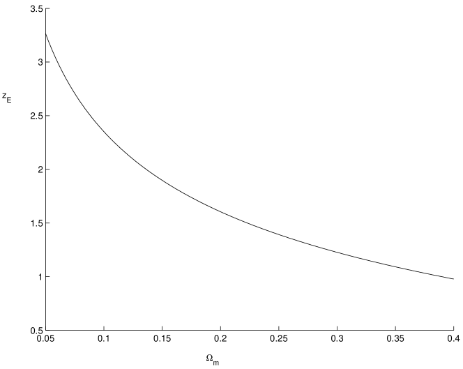
Figure 1: The dependence of the critical redshift $z_{E}$ which characterizes the valid region of perturbation expansion of the field equations on the matter energy density fraction $\Omega_{m}$

The dependence of $z_{E}$ on $\Omega_{m}$ is drawn in Fig.1. In particular, $\Omega_{m}=0.1,0.2,0.3$ gives $z_{E}=2.351,1.603,1.226$ respectively. We will use these values in the following discussions. Thus, the first order Modified Friedmann equation is at most a good approximation to the full field equation up to, e.g. in the case of $\Omega_{m}=0.3$, about redshift 1. We want to know up to what redshift first order approximation is good enough. This is not so obvious, because when $z\sim 1$, $\kappa T/\alpha\sim 0.73$. This is not very small, thus the effects of higher order terms in perturbation expansion may not be negligible when apply the MF equation on these redshift close to $z_{E}$. Future high redshift supernova observations would reach such high redshift region so the behavior of the MF equation in these region is important. On the other hand, if we find that the first order equation is doing good in describing our Universe’s evolution up to redshift $z_{E}$ and the second order correction is small, this is a strong indication that the full field equations also behave well in describing the cosmological evolution. In the below we will see that the effects of the second correction is rather interesting: the first order equation fits the SNe Ia data in an acceptable level and the second order correction is negligible up to the critical redshift $z_{E}$. But the second order effects can not be neglected in describing the acceleration rate, i.e. the deceleration parameter. Thus we have good reason to believe the full field equation is also good in fitting the supernova data and this modified gravity theory may be a good candidate for explanation of the cosmic acceleration.

Thus in order to investigate the valid region of the first order approximation, let us consider the second order approximation to the theory.

First, the scalar curvature can be obtained from eq.(10)

$$R\simeq\alpha[-1+\frac{\kappa T}{2\alpha}-\frac{1}{8}(\frac{\kappa T}{\alpha})^{2}]$$ (22)

From eq.(8):

$$L\simeq\alpha[-\frac{2}{3}+\frac{2}{3}\frac{\kappa T}{\alpha}-\frac{1}{12}(\frac{\kappa T}{\alpha})^{2}]$$ (23)

$$L^{\prime}\simeq\frac{4}{3}[1+\frac{\kappa T}{4\alpha}+\frac{1}{8}(\frac{\kappa T}{\alpha})^{2}]$$ (24)

The second order field equation can be obtained from eq.(9)

$$R_{\mu\nu}=-\frac{1}{4}\alpha g_{\mu\nu}-\kappa[\frac{3}{4}T_{\mu\nu}-\frac{5}{16}Tg_{\mu\nu}]+\frac{\kappa^{2}T}{4\alpha}[\frac{3}{4}T_{\mu\nu}-\frac{5}{16}Tg_{\mu\nu}]$$ (25)

The non-vanishing component of Ricci curvature tensor up to second order is obtained from eq.(5)

$$R_{00}=3\frac{\ddot{a}}{a}+\frac{3}{8}\frac{\kappa\ddot{T}}{\alpha}+\frac{15}{64}(\frac{\kappa\dot{T}}{\alpha})^{2}+\frac{9}{32}\frac{\kappa T}{\alpha}\frac{\kappa\ddot{T}}{\alpha}$$ (26)

$$R_{ij}=-[a\ddot{a}+2\dot{a}^{2}+\frac{a\dot{a}}{4}\frac{\kappa\dot{T}}{\alpha}+\frac{a^{2}}{8}\frac{\kappa\ddot{T}}{\alpha}+\frac{9a^{2}}{64}(\frac{\kappa\dot{T}}{\alpha})^{2}+\frac{3a\dot{a}}{16}\frac{\kappa T}{\alpha}\frac{\kappa\dot{T}}{\alpha}+\frac{3a^{2}}{32}\frac{\kappa T}{\alpha}\frac{\kappa\ddot{T}}{\alpha}]\delta_{ij}$$ (27)

The second order Modified Friedmann equation now follows from equations (26), (27) and (25):

$$H^{2}=\frac{\frac{11}{8}\kappa\rho+\frac{11}{32}\frac{(\kappa\rho)^{2}}{\alpha}+\frac{\alpha}{2}}{6+\frac{9}{4}\frac{\kappa\rho}{\alpha}}$$ (28)

The only correction to the first order equation is the quadratic term in the numerator. It is interesting to note that while the first order MF equation is formally similar to the Friedmann equation in the $\Lambda$CDM model, the second order MF equation is formally similar to the modified Friedmann equation in the RS II brane world cosmology model with an effective cosmological constant Wang .

In terms of the $z_{E}$ defined above, eq.(28) can be rewritten as

$$H^{2}=H_{0}^{2}\Omega_{m}\frac{\frac{11}{8}(1+z)^{3}+\frac{11}{32}\frac{(1+z)^{6}}{(1+z_{E})^{3}}+\frac{1}{2}(1+z_{E})^{3}}{2+\frac{3}{4}(\frac{1+z}{1+z_{E}})^{3}}$$ (29)

Set $z=0$ in eq.(29) gives

$$z_{E}=(\frac{\frac{11}{8}\Omega_{m}-2+\sqrt{(\frac{11}{8}\Omega_{m}-2)^{2}+(\frac{3}{2}-\frac{11}{16}\Omega_{m})\Omega_{m}}}{3/2-\frac{11}{16}\Omega_{m}})^{-\frac{1}{3}}-1$$ (30)

The dependence of $z_{E}$ on $\Omega_{m}$ is almost identical to the first order equation. The difference is very small and is of about order $10^{-4}$.

3. Data Fitting with SNe Ia Observations

It is the observations of the SNe Ia that first reveal our Universe is in an accelerating phase. It is still the most important evidence for acceleration and the best discriminator between different models to explain the acceleration. Thus, any model attempting to explain the acceleration should fit the SNe Ia data as the basic requirement.

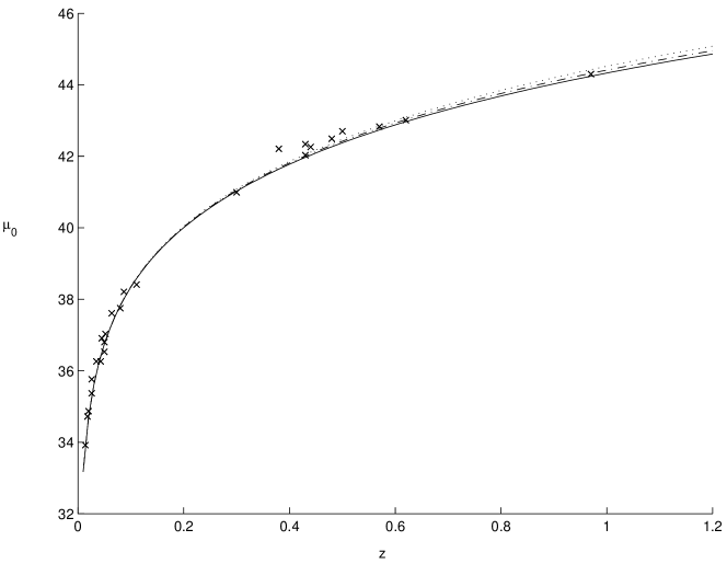
Figure 2: The dependence of luminosity distance on redshift computed from the first order modified Friedmann equation. The dotted, dashed and solid lines correspond to $\Omega_{m}=0.1,0.2,0.3$, respectively. The little crosses are the observed data

Figure 3: The difference between the luminosity distances computed from the first order and second order modified Friedmann equations. The dotted, dashed and solid lines correspond to $\Omega_{m}=0.1,0.2,0.3$, respectively. The difference is very small even up to high redshift larger than 1 which is the upper limit for the validity of perturbation expansion of the full field equation. It shows that we can trust the prediction of first order equation in calculating luminosity distance in almost all the redshift region smaller than the critical value $z_{E}$.

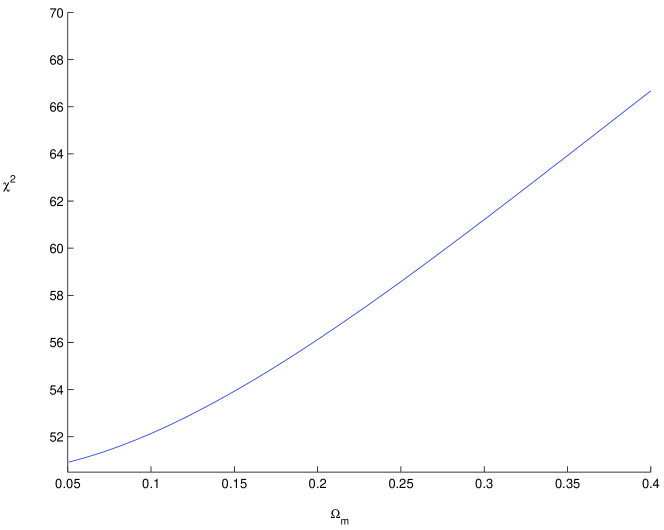
Figure 4: The dependence of the $\chi^{2}$ on the parameter $\Omega_{m}$. It can be seen that $\chi^{2}$ gets a little smaller for smaller value of $\Omega_{m}$.

The supernova observation is essentially a determination of redshift-luminosity distance relationship. The luminosity distance is obtained by a standard procedure:

$$D_{L}=(1+z)r=(1+z)\int_{0}^{z}\frac{dz^{\prime}}{H(z^{\prime})}$$ (31)

where $H(z)$ is given by eq.(20) or eq.(29) for first order and second order approximation respectively.

In the data fitting, we actually compute the quantity,

$$\mu_{0}=5\log(\frac{D_{L}}{Mpc})+25$$ (32)

The quality of the fitting is characterized by the parameter:

$$\chi^{2}=\sum_{i}\frac{[\mu_{0,i}^{o}-\mu_{0,i}^{t}]^{2}}{\sigma_{\mu_{0},i}^{2}+\sigma^{2}_{mz,i}}$$ (33)

where $\mu_{0,i}^{o}$ is the observed value, $\mu_{0,i}^{t}$ is the value calculated through the model described above, $\sigma^{2}_{\mu_{0},i}$ is the measurement error, $\sigma^{2}_{mz,i}$ is dispersion in the distance modulus due to the dispersion in galaxy redshift caused by peculiar velocities. This quantity will be taken as

$$\sigma_{mz}=\frac{\partial\log D_{L}}{\partial z}\sigma_{z}$$ (34)

where following ref.Perlmutter , $\sigma_{z}=200km/s$. We use data listed in ref.Fabris , which contains 25 SNe Ia observations. Since our purpose is to show that first order approximation fits the data at an acceptable level and second order effects can be ignored even up to high redshift such as 1, also because trustable observations around redshift 1 is very few, we think 25 low redshift samples is enough. Also we do not perform a detailed $\chi^{2}$ analysis, this is suitable when we get more high redshift samples.

Fig.2 shows the prediction of the first order MF equation for $\Omega_{m}=0.1,0.2,0.3$ respectively.

Fig.3 draws the difference between the $\mu_{0}$ computed using first and second order MF equations for $\Omega_{m}=0.1,0.2,0.3$ respectively. The prediction of second order MF equation is almost indistinguishable from the first order equation up to redshift 1. The difference is about the order $10^{-2}$ even up to redshift 1. So we did not draw the corresponding luminosity distance curves for second order approximation. And this confirms the assertion we made above. We do can trust that the predictions made by the first order equation in calculating the luminosity distances are good approximation to the full field equations even up to high redshift, just not exceeding the critical redshift $z_{E}$.

Fig.4 shows the dependence of the $\chi^{2}$ computed using eq.(33) on the $\Omega_{m}$. We can see that $\chi^{2}$ gets a little smaller for smaller value of $\Omega_{m}$. We think this is an interesting feature of this modified gravity theory: It has already provide the possibility of eliminating the necessity for dark energy for explanation of cosmic acceleration, now it can be consistent with the SNe Ia observations without the assumption of dark matter. Thus we boldly suggest that maybe this modified gravity theory can provide the possibility of eliminating dark matter (There have been some efforts in this direction, see ref.Milgrom ). This is surely an interesting thing and worth some investigations.

However, we should also note that we only use SNe Ia data smaller than redshift 1 to draw the above conclusions. It can easily been seen in Fig.2 that the differences between predictions drawn from the different values of $\Omega_{m}$ become larger when redshift is around 1. Thus, future high redshift supernova observations may give a more conclusive discrimination between the parameters.

4. The Deceleration Parameter

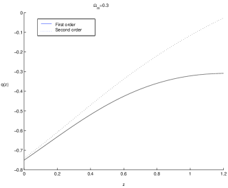
Figure 5: The dependence of the deceleration parameter $q(z)$ on redshift $z$ for $\Omega_{m}=0.1,0.2,0.3$ respectively. The second order effects is seen to be large.

Given the observation that our Universe is currently expanding in an accelerating phase, the deceleration parameter should become negative in recent cosmological times. The deceleration parameter is defined by $q=-\ddot{a}/(aH^{2})$.

In the case of first order approximation, from eq.(19) we can get

$$q=\frac{\frac{21}{16}\frac{\kappa\rho}{\alpha}-\frac{99}{32}(\frac{\kappa\rho}{\alpha})^{2}-3}{(6+\frac{9}{4}\frac{\kappa\rho}{\alpha})(\frac{11}{8}\frac{\kappa\rho}{\alpha}+\frac{1}{2})}$$ (35)

In the case of second order approximation, from eq.(28) we can get

$$q=\frac{\frac{21}{16}\frac{\kappa\rho}{\alpha}+\frac{33}{32}(\frac{\kappa\rho}{\alpha})^{2}+\frac{99}{256}(\frac{\kappa\rho}{\alpha})^{3}-3}{(6+\frac{9}{4}\frac{\kappa\rho}{\alpha})(\frac{11}{8}\frac{\kappa\rho}{\alpha}+\frac{11}{32}(\frac{\kappa\rho}{\alpha})^{2}+\frac{1}{2})}$$ (36)

Since $\kappa\rho/\alpha=(1+z)^{3}/(1+z_{E})^{3}$, we can get the dependence of $q(z)$ on redshift, this is shown in Fig.5. It can be seen that the second order effects can not be neglected for all the three values of $\Omega_{m}$.

Combined with the result of Sec.3, we can draw the conclusion that the second order effects can be neglected on the cosmological predictions involving only the Hubble parameter itself, e.g. the various cosmological distances, but the second order effect can not be neglected in the predictions involving the derivatives of the Hubble parameter. This later assertion can also be confirmed by deriving the effective equation of state of this modified gravity theory.

5. The Effective Equation of State

In this modified gravity theory, following the general framework of Linder and Jenkins Linder , we can define the effective Equation of State (EOS) of dark energy. Written in this form, it also has the advantage that many parametrization works that have been done for EOS of dark energy can be compared with the modified gravity.

Now following Linder and Jenkins, the additional term in Modified Friedmann equation really just describes our ignorance concerning the physical mechanism leading to the observed effect of acceleration. Let us take a empirical approach, we just write the Friedmann equation formerly as

$$H^{2}/H_{0}^{2}=\Omega_{m}(1+z)^{3}+\delta H^{2}/H_{0}^{2}$$ (37)

where we now encapsulate any modification to the standard Friedmann equation in the last term, regardless of its nature.

Define the effective EOS $\omega_{eff}(z)$ as

$$\omega_{eff}(z)=-1+\frac{1}{3}\frac{d\ln\delta H^{2}}{d\ln(1+z)}$$ (38)

Then in terms of $\omega_{eff}$, equation eq.(37) can be written as

$$H^{2}/H_{0}^{2}=\Omega_{m}(1+z)^{3}+(1-\Omega_{m})e^{3\int_{0}^{z}{d\ln(1+z^{\prime})[1+\omega_{eff}(z^{\prime})]}}$$ (39)

Using the above formalism, we can compute the effective equation of state corresponding to the first and second order approximations.

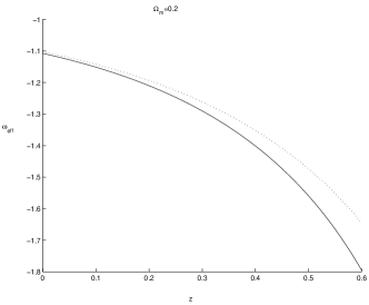
Figure 6: The dependence of the effective equation of state $\omega_{eff}$ on redshift $z$ in the case of $\Omega_{m}=0.1,0.2,0.3$ respectively. Solid and dotted lines correspond to first and second order MF equations respectively. The second order effects is seen to be large.

The first order EOS:

$$\omega_{eff}^{1}=-1-\frac{\frac{9}{16}(\frac{1+z}{1+z_{E}})^{9}+3(\frac{1+z}{1+z_{E}})^{6}+\frac{13}{8}(\frac{1+z}{1+z_{E}})^{3}}{(-\frac{3}{4}(\frac{1+z}{1+z_{E}})^{6}-\frac{5}{8}(\frac{1+z}{1+z_{E}})^{3}+\frac{1}{2})(2+\frac{3}{4}(\frac{1+z}{1+z_{E}})^{3})}$$ (40)

The second order EOS:

$$\omega_{eff}^{2}=-1-\frac{13}{8}\frac{\frac{3}{16}(\frac{1+z}{1+z_{E}})^{9}+(\frac{1+z}{1+z_{E}})^{6}+(\frac{1+z}{1+z_{E}})^{3}}{(-\frac{13}{32}(\frac{1+z}{1+z_{E}})^{6}-\frac{5}{8}(\frac{1+z}{1+z_{E}})^{3}+\frac{1}{2})(2+\frac{3}{4}(\frac{1+z}{1+z_{E}})^{3})}$$ (41)

These two EOSs are drawn in Fig.6. The difference is quite obvious. Furthermore, they diverge before $z_{E}$. Concretely, the first order EOSs diverge at roughly $z=1.65,1.05,0.75$ for $\Omega_{m}=0.1,0.2,0.3$ respectively; the second order EOSs diverge at roughly $z=1.8,1.15,0.85$ for $\Omega_{m}=0.1,0.2,0.3$ respectively. In summary, for higher value of $\Omega_{m}$, the divergence is more rapid and the first order EOS diverges more rapid than second order EOS for the same $\Omega_{m}$, which indicate that second order EOS is a better approximation to the full effective EOS. But we do not know whether the EOS computed from the full field equations also undergo such a divergence. Maybe this divergence is only an indication of the breakdown of perturbation approximation. Note $w_{eff}<1$, which is also a possible behavior of EOS, see ref.Carroll2 .

6. Discussions and Conclusions.

Applying Palatini formalism to the modified Einstein-Hilbert action is an interesting approach that is worth further investigations. In particular, it is free of the sort of instability encountered in the metric variation formalism as argued by Dolgov et. al. Dolgov . And more importantly, we have showed that the MF equations fit the SNe Ia data at an acceptable level. In order to compute other cosmological parameters such as the age of the universe, we need the full MF equation, which has been investigated by us elsewhere Wang3 . It is shown there that the age of the universe is compatible with the age of the globular agglomerates observed today.

We have discussed the effects of second order approximation. We showed that the second order effects can be neglected on the cosmological predictions involved only the Hubble parameter itself, e.g. the various cosmological distances, but the second order effects are large in the predictions involved the derivatives of the Hubble parameter. Thus, in the future work dedicated to discuss the cosmological effects or local gravity effects of this modified gravity theory, second order MF equation (28) seems a better starting point. Of course, whether the effects of third order effects or even the non-perturbative effects can not be negligible in redshift smaller than $z_{E}$ for some situations deserve further investigations.

In summary, adding a $R^{-1}$ or the like terms to the Einstein-Hilbert action is an interesting idea, which may originate from some Sring/M-theory jap , and looks like a possible candidate for the explanation of recent cosmic expansion acceleration fact. We can see such modifications may accommodate the update observational data indicating our Universe expansion is accelerating without introducing the mysterious so called Dark Energy. However, so far as we know the update experimental testings to General Relativity Gravity theory within the Solar system data have repeatedly confirmed that the GR is right; now for larger cosmic scale if we should modify the conventional gravity theory to confront cosmological observations, it is vital to both our basic understanding of the Universe and development for fundamental physical theories.

Acknowledgements

We would like to thank the referees’ very helpful comments which have improved this paper greatly. P.W. wishes to thank Professor A. Lue and R. Scoccimarro for valuable discussions. X.H.M. has benefitted a lot by helpful discussions with R.Branderberger, D.Lyth, A.Mazumdar, L.Ryder, X.P.Wu, K.Yamamoto and Y. Zhang. This work is partly supported by China NSF, Doctor Foundation of National Education Ministry and ICSC-world lab. scholarship.

References

- (1) S. Perlmutter el al. Nature 404 (2000) 955; Astroph. J. 517 (1999) 565; A. Riess et al. Astroph. J. 116 (1998) 1009; ibid. 560 (2001) 49; Y. Wang, Astroph. J. 536 (2000) 531;
- (2) D.N.Spergel, et al., astro-ph/0302207; L.Page et al. astro-ph/0302220; M.Nolta, et al, astro-ph/0305097; C.Bennett, et al, astro-ph/0302209;
- (3) P. J. E. Peebles, B. Ratra, astro-ph/0207347;
- (4) R. R. Caldwell, R. Dave and P. J. Steinhardt, Phys. Rev. Lett. 80 (1998) 1582;
- (5) A. Kamenshchik, U. Moschella and V. Pasquier, Phys. Lett. B511 (2001) 265;
- (6) A. Lue, R. Scoccimarro and G. Starkman, astro-ph/0307034;
- (7) G. Dvali, G. Gabadadze and M. Porrati, Phys. Lett. B485 (2000) 208;
- (8) S. M. Carroll, V.Duvvuri, M.Trodden and M. Turner, astro-ph/0306438;
- (9) S. Capozziello, S. Carloni and A. Troisi, ”Recent Research Developments in Astronomy & Astrophysics” -RSP/AA/21-2003 [astro-ph/0303041]; S.Capozziello, Int.J.Mod.Phys.D 11 (2002) 483;
- (10) S.Capozziello et al., astro-ph/0307018;
- (11) D. N. Vollick, astro-ph/0306630;
- (12) A. D. Dolgov and M. Kawasaki, astro-ph/0307285;
- (13) A.R.Lidde and D.H.Lyth, Cosmological Inflation and Large Scale Structure, Cambrigde University Press, 2000;
- (14) X.H.Meng, P.Wang and W.Y.Zhao, to appear in Int.J.Mod. Phys.D; L.Randall and R.Sundrum, Phys.Rev.Lett.83 (1999)3370; ibid.83(1999)4690; P.Binetruy, C.Deffayet, U.Ellwanger and D.Langois, Phys. Lett. B477 (2000) 285;
- (15) J. C. Fabris, S. V. B. Goncalves and P. E. de Souza, astro-ph/0207430;
- (16) M. Milgrom, Astrophys. J. 270 (1983) 365; R. H. Sanders and S. S. McGaugh, Annual Review of Astronomy and Astrophysics Sep 10 (2002) 263 [astro-ph/0204521];
- (17) E. V. Linder and A. Jenkins, astro-ph/0305286;
- (18) S. M. Carroll, M. Hoffman and M. Trodden, astro-ph/0301273;
- (19) X.H.Meng and P.Wang, astro-ph/0308031;
- (20) S. Nojiri and S. D. Odintsov, hep-th/0307071;
- (21) Paticle Data Group. K. Hagiwara et al., Phys. Rev. D66 (2002) 010001; C. M. Will, Theory and Experiment in Gravitational Physics (Cambridge Universtiy Press, Cambridge,1993); Living Rev. Rel. 4 (2001) 4;