XMM-Newton observation of the interacting cluster Abell 3528

We analyze the XMM-Newton dataset of the interacting cluster of galaxies Abell 3528 located westward in the core of the Shapley Supercluster, the largest concentration of mass in the nearby Universe. A3528 is formed by two interacting clumps (A3528-N at North and A3528-S at South) separated by 0.9 $h_{70}^{-1}$ Mpc at redshift 0.053. XMM-Newton data describe these clumps as relaxed structure with an overall temperature of $4.14\pm 0.09$ and $4.29\pm 0.07$ keV in A3528-N and A3528-S, respectively, and a core cooler by a factor 1.4–1.5 and super-solar metal abundance in the inner 30 arcsec. These clumps are connected by a X-ray soft, bridge-like emission and present asymmetric surface brightness with significant excess in the North–West region of A3528-N and in the North–East area of A3528-S. However, we do not observe any evidence of shock heated gas, both in the surface brightness and in the temperature map. Considering also that the optical light distribution is more concentrated around A3528-N and makes A3528-S barely detectable, we do not find support to the originally suggested head-on pre-merging scenario and conclude that A3528 is in a off-axis post-merging phase, where the closest cores encounter happened about 1–2 Gyrs ago.

1 Introduction

Clusters of galaxies are thought to form by accretion and merging of subunits in a hierarchical bottom-up scenario. Numerical simulations on scales of cosmological relevance revealed that mergings happen along preferential directions, called density caustics, which define matter flow regions, at whose intersection rich clusters are formed (Cen & Ostriker 1994, Colberg et al. 1999). Cluster mergings are therefore the most common and energetic phenomena in the Universe, leading to an energy release of as much as $10^{64}$ ergs on a timescale of the order of Gyrs, whose astrophysical consequences are expected to be both thermal (presence of shocks, changes in the temperature and gas distribution of the Intra Cluster Medium) and non thermal (appearance of radio sources like Halos or Relics) as well as influences on the galaxy population (presence of starbust galaxies, wide angle tail radiosources) (see Sarazin 2002, Girardi & Biviano 2002, Buote 2002, Böhringer & Schuecker 2002, Forman et al. 2002, Feretti & Venturi 2002, Giovannini & Feretti 2002). The understanding of cluster merging thus needs a full multi wavelength analysis (optical, radio and X-ray) in order to have a more global view of the phenomenon and the improvement and extension of available data. For the second issue the advent of the new generation of X-ray observatories is giving a lot of results, as Chandra reveled with the long seeked first clear example of bow shock in the ICM (Markevitch et al. 2002), the most prominent feature seen in cluster merging simulations (see Schindler 2002 for a review), and the discovery of the completely unexpected phenomenon of cold fronts, which are direct consequences of the survival of cluster cores during the process of merging, at least in the most spectacular cases of A3667 and A2142 (Vikhlinin et al. 2001, Forman et al. 2002 for a review).

In the same way as the caustics seen in the simulations, rich superclusters are the ideal environment for the detection of cluster mergings, because the peculiar velocities induced by the enhanced local overdensity (of the order of $\sim 10$) of the large-scale structure favor the cluster-cluster collisions. The Shapley Supercluster (Shapley 1930) is the largest concentration of mass within $z=0.1$ (Zucca et al. 1993, Bardelli et al. 1994, Ettori, Fabian & White 1997) with a high local overdensity (of the order of $\sim 10$ on scales of $10\,\rm{h}^{-1}$ Mpc, Bardelli et al. 2000) showing remarkable examples of cluster mergings at various evolutionary stages. In particular, two cluster complexes are found in this concentration, around A3558 in the core and A3528 westward, respectively. These structures, whose spatial scales are of order of $\sim\,5\,\rm{h}^{-1}$ Mpc (Bardelli et al. 2000) are formed by strongly interacting clusters. The complex dominated by A3558 is probably a merging seen just after the first core-core encounter (Bardelli et al. 1998, Hanami et al. 1999). The other complex is formed by the ACO (Abell, Corwin & Olowin 1989) clusters A3528, A3530 and A3532, located northwest of the A3558 complex.
In this paper we concentrate on the XMM-Newton observation of the cluster A3528.

The outline of the paper is as follows. We describe in Sect. 2 the general properties of A3528 and present in Sect. 3 the X-ray spatial and spectral analysis of the XMM-Newton observation. In Sect. 4, we consider the state of the merging how it appears at optical and radio wavelengths. Finally, we discuss and summarize our results in Sect. 5 and Sect. 6, respectively. More details on technical aspects of the X-ray analysis are presented in the Appendices at the end of the paper.

At the nominal redshift of A3528 (z=0.053), 1 arcmin corresponds to 62 kpc ($H_{0}=$ 70 $h_{70}$ km s^-1 Mpc^-1, $\Omega_{\rm m}=1-\Omega_{\Lambda}=$ 0.3). In the following analysis, all the quoted errors are at $1\sigma$ (68.3 per cent level of confidence) unless stated otherwise.

2 The cluster A3528

The cluster A3528 is a Bautz-Morgan type II galaxy cluster with richness of class 1, the highest in the complex being the other two clusters, A3530 and A3532, of richness class 0. Raychaudhury et al. (1991) found, using Einstein IPC, that this cluster is actually double, formed by two subcomponents, A3528-N and A3528-S, centered on the two dominant galaxies clearly visible in the optical, with a likely although poor indication of the presence of a cool core. From a ROSAT pointed PSPC observation, Schindler (1996) showed evidence of interaction, dividing the two subclusters in four semicircles, with the semicircles facing the other subcluster with higher temperatures than the outer ones, suggesting the presence of a shock. Henriksen & Jones (1996) estimated a temperature of $2.7\pm 0.8$ and $2.9\pm 0.9$ keV for A3528-N and A3528-S, respectively, suggesting as unlikely the presence of a cool core in the two subclusters. However this observation is not optimal: the cluster is off-centered respect to the ROSAT pointing and partly obscured by the supporting ribs (see Fig.8 of Reid et al. 1998) and there are some concerns about the capability of the PSPC to obtain accurate temperature determination (Markevitch & Vikhlinin 1997, Ettori et al. 2000).

Optical (Bardelli et al. 2001, Baldi et al. 2001) and radio observations (Reid et al. 1997, Venturi et al. 2001) seem to indicate that the A3528 complex is in a pre-merging phase because the cluster galaxies in the inner regions are not far from the virial equilibrium and their optical and radio properties are not yet affected from merging effects.

Donnelly et al. (2001) using ASCA GIS data found an overall cluster temperature (comprising the two subclusters) of $4.7\pm 0.3$ keV and analyzing five indicative regions (two regions for each subcluster, one around the core and one in the outer region, and a region between the two subclusters, see their Fig.1) provided further support to the idea that A3528 is in the early stages of a merger, where the gas in both subclusters is only just beginning to interact. They claimed (still by ROSAT data) that the cores show evidence of cool gas, the intensity contours are still azimuthally symmetric and the temperature of the gas located between the subclusters is only marginally hotter ($\sim 15\%$) than the overall average for the cluster.

3 X-ray analysis

3.1 Observation and data preparation

Figure 1: Light curves for PN (upper panel) and, for comparison, of the MOS 1 (lower panel) in the band [10-12] keV and the intensity filters we use.

A3528 was observed by XMM-Newton during rev. 374 with the MOS and PN detectors in Full Frame Mode with medium filter, for an exposure time of 16.4 ks for MOS and 14.0 ks for PN. We have obtained calibrated event files for the three EPIC cameras with SASv5.3.3 using the tasks emproc and epproc.
The removal of bright pixels and hot columns was done, especially for the PN, in a conservative way applying the expression (FLAG ==0) to the extraction of spectra and images.
To reject the soft proton flares, we accumulate the light curve in the [10-12] keV band (see comparison in Fig.1), where the emission is dominated by particle induced background: while the MOS camera are not affected by flares (count rates are lower than our intensity threshold, fixed at 15 cts/100s), we observe a flare in the PN detector with a count rate exceeding our limit of 35 cts/100s. Thus, we reject all the PN events related to this flare deriving a total effective exposure time of 11.0 ksec. The pattern selection was [0;12] for MOS cameras and singles events for the PN.

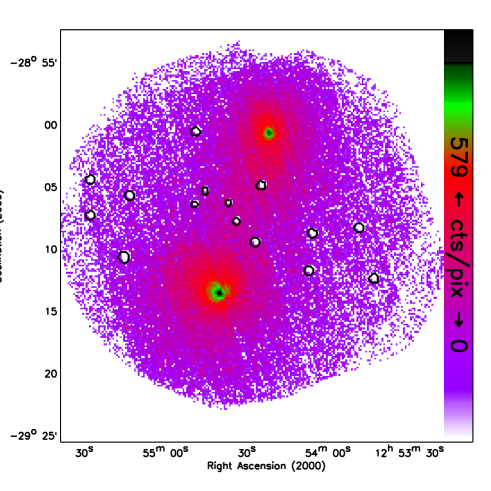
Figure 2: XMM-Newton EPIC image of the cluster A3528 in the band [0.5-10.0] keV. The bright sources detected by the pipeline processing of the image are masked. It is worth noticing the high concentration of these X-ray emitting point sources in the region lying between the two clumps. None of these have an associated redshift.

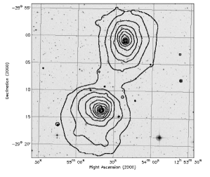
Figure 3: XMM-Newton contour plots of the EPIC image of the cluster A3528 in the band [0.5-10.0] keV superposed on the DSS image, in the Bj band, of the same field of view. The contours are spaced by a factor of $\sim 1.4$ between 1.7 and 579 cts/pixel.

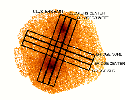
Figure 4: The regions used for the detection of the diffuse emission between the two clumps are here superimposed on the total EPIC raw image. The width of the strip is of 13.2 pixels $\approx 1.90$ arcmin. The surface brightness profiles shown in Fig. 5 are extracted along these strips and are obtained by accumulating the counts in bins of 10 pixels ($\approx 1.44$ arcmin) each. The progression of the bins starts from north to south along the “clusters” regions, while from west to east in the “bridge” regions.

To remove all other background components we do not use blank sky regions as the Lockman Hole observations or the background templates provided by the EPIC team (Lumb 2002), because all these fields are observed with thin filter and with low levels of galactic absorption. We prefer to use as background the long observation (100 ks) of the quasar APM 08279+5255 (Hasinger et al. 2002) performed with medium filter, which has also a Galactic $\rm{N_{H}}$ of $4\times 10^{20}\,\rm{cm^{-2}}$ more similar to the one in the direction of A3528 ($6.1\times 10^{20}\,\rm{cm^{-2}}$). We performed the same selection criteria for the background as the source, we removed all the bright sources and after rejection of soft proton flares we got an effective exposure time of 73 ks for MOS and 62 ks for PN. We reprojected the background field to the same sky coordinates of the source by means of the SAS task attcalc and then performed the background subtraction in sky coordinates.

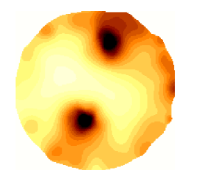
Figure 5: (Left) Adaptively smoothed exposure corrected EPIC image of A3528 in the soft ([0.5-2.0] keV; top panel), medium ([2.0-4.5] keV, middle panel) and hard band ([4.5-8.0] keV, bottom panel). (Right) Count rates in the regions defined in Fig.4 and obtained in the soft ([0.5-2.0] keV; top panel), medium ([2.0-4.5] keV; middle panel) and hard ([4.5-8.0] keV; bottom panel) band. The error bars are the 1$\sigma$ Poisson errors and the background shown as a dotted line is obtained by a median of the counts in the two last bins West and East of the three “bridge” regions. Each bin has dimension 13.2$\times$10 pixels² ($\approx 1.90\times 1.44$ arcmin²; see caption of Fig. 4).

We perform (and cross-check) the vignetting correction in two independent ways: by applying it to (i) the spectra as is customary in the analysis of EPIC data (Arnaud et al. 2001, Gastaldelo & Molendi 2002) and (ii) the effective area via the use of the ancillary response file (arf) created through the SAS task arfgen.

3.2 Spatial analysis

We use the clean linearized event files to generate MOS 1, MOS 2 and PN images in the energy band [0.5-10] keV with a spatial binning of 8 arcseconds per pixel. We merge together the three cameras images in order to increase the signal-to-noise ratio and the result is shown in Fig.2. In Fig.3 we show the logarithmically spaced contour plots obtained by the source cleaned EPIC image in the band [0.5-10.0] keV superposed on the optical DSS image. The two clumps, A3528-N and A3528-S, have a maximum at (RA, Dec, 2000)=$(12^{\rm h}54^{\rm m}22\aas@@fstack{s}1,-29^{\circ}00^{\prime}46^{\prime\prime})$ and $(12^{\rm h}54^{\rm m}40\aas@@fstack{s}6,-29^{\circ}13^{\prime}44^{\prime\prime})$, respectively, with a comoving separation of 0.90 $h_{70}^{-1}$ Mpc (a redshift of 0.053 is assumed for both the subclusters).

A diffuse faint emission appears to connect the two clumps. In order to check the significance of this diffuse emission, we perform an analysis of the counts along the regions depicted in Fig.4. We do this on EPIC images generated in three different energy bands, soft (0.5-2.0 keV), medium (2.0-4.5 keV) and hard (4.5-8.0 keV). The corresponding set of exposure maps for each camera has been prepared to account for spatial quantum efficiency, mirror vignetting and field of view of each instrument by running the SAS task eexmap. The images from the three instruments are then merged, weighting each of these by the ratio of its maximum exposure time to the total maximum exposure time. We restrict the higher bound of the hard energy band to avoid effects from vignetting over-correction due to the prevalence of the flat instrumental background in the broader energy band 4.5-10 keV. We do not consider regions exposed less than 10% of the total exposure. From these exposure-corrected images, we obtain the surface brightness profiles in the six regions marked in Fig.4. These profiles are shown in Fig.5 with the corresponding adaptively smoothed, exposure corrected images in the three energy bands adopted. The CIAO tool csmooth, set to a minimum signal to noise ratio of 3, is used to produce these images. The marked regions were choosen with the idea of looking for the enhancement of counts along the “bridge” regions above the background. We use three regions along the same directions to quantify the variations along the East-West and North-South directions of the diffuse emission. Obviously the significance of plotting “bridge” and “cluster” regions together stands in the overlap regions, where the bin have the same location. A significant excess with respect to the background is detected between the clumps in the soft and medium exposure-corrected images, while on the contrary no excess is observed in the hard image. In the hard band image, some edge effects cannot be avoided due to the low statistic and the level of background.

3.3 Spectral analysis

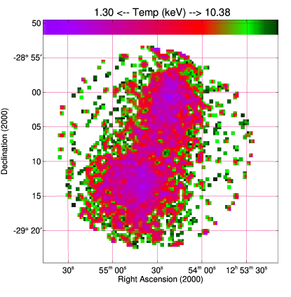
Figure 6: Temperature map obtained by using 5 X-ray colours (0.4–0.8, 0.8–1.4, 1.4–2.0, 2.0–4.5, 4.5–8.0 keV) and estimating the expected count rate with XSPEC for a thermal MEKAL model, with fixed Galactic absorption $\rm{N_{H}}\,$and metallicity. The observed count rate is estimated in $4\times 4$ original bins of $(8.7\times 8.7)$ arcsec² with step in X and Y of $2$ bins.

We refer to Appendix A for details on the calibration issues we deal with during our analysis. We focus here on the method used and the scientific results obtained.

The spectral analysis has been performed in successive steps. From X-ray colours, we build a temperature map (see Fig. 6) that we use to individuate interesting regions for further analysis. The two clumps appear to have temperature between $2$ and $4$ keV moving outward and do not show significant enhancement in temperature in the region between them. We then consider circles of 6 arcmins in radius centered on each cluster’s emission peak. We use a MEKAL (Mewe et al. 1985; Liedahl et al. 1995) model in XSPEC (v.11.1.0, Arnaud 1996) leaving as free parameters the column density $\rm{N_{H}}$, the intracluster temperature $\rm{kT}$, the metallicity $\rm{Z}$ (in solar unity with respect to the values quoted in Grevesse & Sauval 1998), the redshift z and the normalization. A3528 is at an optical redshift of 0.053 and the column density along the line of sight is $\rm{N_{H}}=6.1\times 10^{20}\,\rm{cm^{-2}}$. The results are shown in Tab.1 in Appendix B where in the upper half we show the results obtained using the effective area files, while in the bottom half the results obtained performing the vignetting correction directly on the events. We confirm that the two methods agree well and adopt the one that performs vignetting correction via the creation of an arf file in the analysis that follows.

     

Figure 7: Temperature (upper panels) and metal abundance (lower panels) profiles for A3528-N and A3528-S. The dots show the best-fit results, while the squares are the deprojected values. The horizontal bars represent the width of the bins used to extract the counts and the dotted line indicates the temperature value from a spatially integrated fit. Uncertainties are at the 68% level for one interesting parameter ($\Delta\chi^{2}=1$.)

Figure 8: EPIC temperature map (left) and abundance map (right).

Figure 9: Gas temperature (upper panels) and metal abundance (lower panels) profiles measured in $90\deg-$sectors for A3528-N (left) and A3528-S (right). Uncertainties are at the 68% level for one interesting parameter ($\Delta\chi^{2}=1$).

We try to correct for the uncertainties related to calibration and background subtraction (see Appendix) in a step-by-step procedure. We fix the $\rm{N_{H}}\,$at the Galactic value and the redshift at the optical determination and measure temperature and abundances in different spectral bands (in function of the low energy cutoff, having found that different high energy cutoff, i.e. 8, 9 and 10 keV, has no effects on the temperature determination) and adopting different recipes for the background subtraction. We first use the plain background, in a second step we renormalize the background levels for different levels of intensity in the hard band ([8-12] keV) and in a last step we apply the double subtraction method, described in Appendix A of Arnaud et al. (2002).

For what concern the background, we are in condition to asses all its relevant components: the particle induced background is monitored in the hard part of the spectrum ($>$ 8 keV) and its count rate checked in order to renormalize the background field at the same count rate level; moreover, the large area free of sources emission in our observation allows to perform the double background subtraction and to take control of the soft component of the cosmic X-ray background, that is estimated to be 75% higher in the direction towards A3528 than towards our reference background field, APM 08279+5255, (see ROSAT survey maps through HEASARC X-ray background tool, Snowden et al. 1997). To do that, we consider two circular regions of 3 arcmin-diameter to the West and East of A3528 and free of cluster emission, estimate the local background and compare it with what measured in the corresponding regions of the blank field reprojected on the same sky coordinates. The count rate level in the hard X-ray band (8-12 keV) are: for MOS1 we have $2.06\pm 0.12\times 10^{-2}\,\rm{cts\,s^{-1}}$ for the source and $1.79\pm 0.05\times 10^{-2}\,\rm{cts\,s^{-1}}$ for the blank sky observation, for MOS2 $1.98\pm 0.12\times 10^{-2}\,\rm{cts\,s^{-1}}$ for the source and $1.88\pm 0.05\times 10^{-2}\,\rm{cts\,s^{-1}}$ for the background and for PN singles $5.86\pm 0.31\times 10^{-2}\,\rm{cts\,s^{-1}}$ and $5.22\pm 0.09\times 10^{-2}\,\rm{cts\,s^{-1}}$. We then use a normalization factor of 1.15 for MOS1, 1.05 for MOS2 and 1.12 for the PN.

The results with different levels of background subtraction and different fitting energy bands are shown in Appendix C (cf. Fig.15). By using the double subtraction method, which takes in principle all the components of the background into account, and a joint fit of the three cameras, we measure an emission-weighted temperatures within the inner 6 arcmin of $4.14\pm 0.09$ keV for A3528-N and $4.29\pm 0.07$ keV for A3528-S (the fits are performed in the [0.5-8] keV band with galactic absorption $\rm{N_{H}}\,$and redshift fixed). The overall abundances are $0.62\pm 0.05$ $Z_{\odot}$for A3528-N and $0.45\pm 0.04$ $Z_{\odot}$ for A3528-S (reduced $\chi^{2}$ of 1.13 for 892 degrees of freedom and 1.05 for 1038 d.o.f. for A3528-N and A3528-S, respectively).

We then analyze temperature and abundance profiles for the two subcluster performing the same steps as for the global analysis. The two subcluster emissions have been divided into four concentric annuli with bounding radii $0^{\prime}-0.5^{\prime}$, $0.5^{\prime}-1.5^{\prime}$, $1.5^{\prime}-3^{\prime}$ and $3^{\prime}-6^{\prime}$. We fit a single temperature model with fixed $\rm{N_{H}}\,$and redshift to all the spectra. We show in Figure 9 the temperature and abundance profiles obtained by using the double subtraction and a joint fit of the three cameras in the energy band 0.5-8.0 keV (the profiles for each EPIC camera are shown in Appendix C). All the spectra can be properly fitted with a single temperature model, including the innermost bins ($\chi^{2}=210$ for 191 d.o.f. and $\chi^{2}=298$ for 287 d.o.f. for the central bins of A3528-N and A3528-S, respectively). The fits are not improved by adding another thermal component.

The two subclusters show clear evidence of a cool core, with a peaked surface brightness and a steep gradient in metal abundance, the latter being more strong in A3528-N (see Fig. 7). An estimate of the cooling time, $t_{\rm cool}\approx(3/2)n_{\rm gas}T_{\rm gas}\times Vol/L_{\rm X,bol}$, in the inner 30 $h_{70}^{-1}$ kpc of A3528-N and A3528-S gives values of 0.8 and 1.2 Gyr, respectively, an order of magnitude lower than the expected age of the Universe at $z=0.053$ (12.7 Gyr).

With XMM we can provide a detailed temperature map and in particular study in greater detail the northern subcluster and directly the region between the two subclusters, which were affected by the ROSAT supporting structure (see Fig.8 of Reid et al. (1998)). We fit the EPIC cameras together since the beginning, in order to increase the signal to noise ratio, fixing the band at [0.5-8.0] keV and with $\rm{N_{H}}\,$and redshift fixed. We divide each annular region analyzed before in four angular sectors 90 degrees wide and in addition we analyze three central boxes of $6\times 1$ arcmin in the region between the two subclusters, to address the presence of any increase in the temperature due to shocks. In all the regions used we have more than 70% of source counts. The results are shown in EPIC temperature and abundance maps in Fig.8. In Fig.9, the temperature and abundance profiles in the four sectors are shown for A3528-N and A3528-S. The regions between the two clusters show no evidence of temperature enhancement as the temperature and abundance values in the three central boxes are, going from North to South, $4.46^{+0.61}_{-0.50}$ keV, $3.90^{+0.66}_{-0.60}$ keV, $3.79^{+0.53}_{-0.52}$ keV. The abundances have large errors due to low statistic in the iron line and are $0.27^{+0.37}_{-0.27}$, $0.14^{+0.27}_{-0.14}$, $0.0^{+0.26}_{-0.0}$ $Z_{\odot}$.

4 The state of merging at other wavelengths

4.1 In the optical

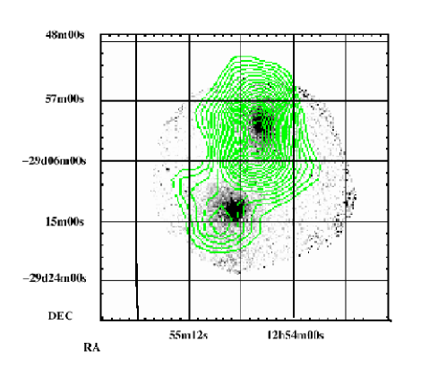
Figure 10: Isodensity distribution of the light in the A3528-N and A3528-S region, from the COSMOS/UKSTJ galaxy catalogue, over plotted onto the X-ray image. These contours have been calculated by summing the galaxy luminosities in bins of $2\times 2$ arcmin and then smoothed with a Gaussian of 3 pixels FWHM.

In the X-ray band, A3528-N and A3528-S appear to be very similar both in luminosity and in mass. On the contrary, considering the distribution of optical galaxies, there is an evident asymmetry between the two subclumps, being A3528-N clearly dominant with respect to A3528-S.

In Fig.10 we show the isodensity contours of the galaxy light from the COSMOS/UKSTJ galaxy catalogue (Yentis et al. 1992), overplotted onto the X-ray image. These contours have been derived by summing the luminosities of galaxies in bins of $2\times 2$ arcmin and then smoothed with a Gaussian of 3 pixels FWHM. This procedure gives more information with respect to a simple number weighted binning, because it takes into account the possibility of a difference in the luminosity distribution of the two clusters.

From this figure it is immediately clear the difference in total luminosity of the two subclumps, being A3528-N about 8.6 times more luminous than A3528-S. Moreover, while there is a good agreement between the position of the peak of the light distribution, the cD galaxy and the X-ray peak in A3528-N, the maximum in the light map of A3528-S is shifted by $\sim 2.8\,\rm{arcmin}$ to the South with respect to the position of the cD galaxy (that coincides with the X-ray peak; see, e.g., Fig. 3). In the case that a merging is taking place along the North-South direction, this shift is in opposition to what expected, with the galaxies that tend to preceed the hot gas (see, e.g., Tormen, Moscardini & Yoshida 2003).

It is quite difficult to explain why these two clumps with very similar X-ray properties appear so different in the optical band. This fact, added to the relative shift between light and hot gas distribution, seems to indicate that an interaction between the more external, non-collisional part of the clusters (the galaxies) is already in place, leading to a loss of optical light in A3528-S. This could be an off-axis merging where the two clusters are orbiting around each other: however, this scenario does not explain why A3528-N, although having the same mass, appears more relaxed. The reason could be a different dynamical history of the two clumps, i.e. A3528-S suffered more than A3528-N of tidal forces during its travel in the A3528 complex.

Unfortunately, no help comes from the velocities, being impossible to divide the contribution of the two clumps (Bardelli et al. 2001): there is only an indication of two peaks in the velocity histograms, corresponding to the velocities of the two cD galaxies (16564 km s^-1 for cD North and 16923 km s^-1 for cD South) but the overall distribution is significantly consistent with a single Gaussian of $\sigma\sim 888$ km s^-1.

4.2 In the radio

The radio properties of A3528-N and A3528-S do not provide strong constraints about the status of the merging in A3528, nevertheless some considerations can be made. The radio luminosity function (RLF) for early–type galaxies, which reflects the probability of an early–type galaxy of given optical magnitude to develop a radio galaxy above a given radio power, is in agreement with the ”universal” RLF for early–type galaxies (Venturi et al. 2001). Even though there is not yet a general consensus on the effect of cluster mergers on the RLF (see for instance Miller & Owen 2003 and Venturi et al. 2002), it is most likely that the RLF in the A3528 complex reflects a virialized situation.

Another striking feature of the radio emission in A3528 is the presence of 5 extended radio galaxies. Three of them are narrow angle tail (NAT) sources and are located at the centre of A3528-N, at the centre of A3528-S and in between them, respectively. In all five cases, multifrequency high resolution radio observations show an active nucleus and twisted/distorted jets and lobes (Venturi et al. in prep). The radio emission associated with the dominant galaxies of A3528-N and A3528-S is all embedded in the optical light, while in the other cases the projected linear size exceeds that of the optical counterpart and limited to $\sim$ 30 – 45 kpc. It is noteworthy that the tails of the two centrally located NATs point in the same direction (South–West to North–East). It is now believed that a combination of ram pressure (due to the galaxy velocity with respect to the intracluster medium) and ”cluster weather” (i.e. bulk motion in the intracluster gas) are the mechanisms responsible for the tail bending (see Feretti & Venturi 2002 for a brief and recent review). Considering that the tails are very short and cluster weather may not be so efficient on such small scales, it is likely that ram pressure is here the dominant mechanism for the formation of the two NATs.

Finally, the lack of indication of extended cluster scale radio emission also deserves a comment. It is now accepted that cluster mergers can provide the necessary electron reacceleration to produce radio halos (see for instance Buote 2002; Giovannini & Feretti 2002; Sarazin 2002 for recent reviews), provided that enough relativistic electrons are deposited in the intracluster medium. Cluster active radio galaxies are the most likely sources of electron replenishment. The high number of active radio galaxies in A3528-N and A3528-S indicates that the presence of relativistic particles is not an issue here, however there is no indication of a radio halo. This may suggest that particle acceleration induced by merger, if present at all in the central regions of two clumps, is not efficient to reaccelerate the electrons at the levels requested to form a radio halo. None of these pieces of evidence is conclusive, however they all seem to suggest that a major merger (or an on–axis merger) between the two structures has not (yet) taken place.

5 Discussion

The two clumps that compound A3528 have the distinctive features of relaxed structures, with a centrally peaked surface brightness (see Fig. 2), a cool core and a steep gradient in metal abundance (see Figs. 7 and 9). A X-ray soft, bridge-like emission (as shown in Fig. 5) connects them. Considering also the absence of characteristic enhancement in the gas temperature both in the X-ray colours (Fig. 6) and spectral (Fig. 8) maps and sharp discontinuities in the surface brightness distribution, we have no indication of shock heated gas and that a merging action is now in progress, at least a major head-on (i.e. impact parameter equals to zero) merger.

Figure 11: Mass profiles of A3528-N and A3528-S (points: from hydrostatic equation applied to the spectral deprojected results; dashed lines: $1\sigma$ range values obtained by assuming a King profile; dotted line $1\sigma$ range values obtained by assuming a NFW profile).

To assess the dynamics of the two subclumps forming A3528, we recover the gravitational mass profiles in these systems by using the deprojected best-fit spectral results obtained for azimuthally averaged annular spectra (see Fig. 7 and details in Ettori, De Grandi, Molendi 2002). Assuming the spherically symmetric distribution of the X-ray emitting plasma in hydrostatic equilibrium with the underlying dark matter potential, we infer a total gravitating mass of $8.0^{+0.7}_{-1.3}\times 10^{13}h_{70}^{-1}M_{\odot}$ and $7.8^{+0.5}_{-0.8}\times 10^{13}h_{70}^{-1}M_{\odot}$ for A3528-N and A3528-S, respectively, within 6 arcmin ($0.38h_{70}^{-1}$ Mpc). We also assume two functional forms of the dark matter potential, the King approximation to the isothermal sphere (Binney and Tremaine 1987) and a Navarro, Frenk & White (NFW) (1997) profile,

$$M_{\rm tot,model}(<r)=4\pi\ r_{\rm s}^{3}\ \rho_{\rm s}\ f(x),$$

$$\rho_{\rm s}=\rho_{\rm c}\frac{200}{3}\frac{c^{3}}{\ln(1+c)-c/(1+c)}$$ , (1)

$$f(x) = \left\{\begin{array}[]{l}\ln(x+\sqrt{1+x^{2}})-\frac{x}{\sqrt{1+x^{2}}}\;{\rm(King)}\\ \ln(1+x)-\frac{x}{1+x}\ \hskip 28.45274pt{\rm(NFW)}\end{array}\right.$$ (3)

where $x=r/r_{\rm s}$, $\rho_{c}$ is the critical density and the relation $r_{\Delta=200}=c\times r_{\rm s}$ holds for the NFW profile. We try to assess which is the mass model that better reproduces the deprojected gas temperature profile by inverting the equation of the hydrostatic equilibrium. We obtain that the King profile is a better modelling of the data ($\chi^{2}=3.9$ and $7.0$ for A3528-N and A3528-S, respectively, whereas a NFW profile gives $7.9$ and $14.9$ for 2 degrees-of-freedom) with best-fit parameters $(r_{\rm s},c)=(86\pm 6$ kpc, $11.2\pm 0.6)$ and $(75\pm 4$ kpc, $13.1\pm 0.5)$ for A3528-N and A3528-S, respectively [$(265\pm 47$ kpc, $5.2\pm 0.6)$ and $(197\pm 26$ kpc, $6.8\pm 0.6)$ for a NFW profile; see Fig. 11]. From the best-fit results of the King profile, we can extrapolate the mass expected in these clumps at an overdensity of 200 with respect to the critical density, and we obtain a total virial mass of $1.5\times 10^{14}h_{70}^{-1}M_{\odot}$ and $1.6\times 10^{14}h_{70}^{-1}M_{\odot}$ for A3528-N and A3528-S, respectively, at about $r_{200}=1.1h_{70}^{-1}$ Mpc. In a simple, but still extreme, scenario in which the two systems lie on the plane of the sky, with the apparent distance between the centers of 0.9 $h_{70}^{-1}$ Mpc being their 3D spatial separation, and are falling from infinity with zero angular momentum and zero initial velocity toward each other, their relative velocity, $v=\sqrt{2G(M_{1}+M_{2})/R}$, should be of $\sim$1720 km s^-1 and their centers should cross in about 0.5 Gyr. This infall velocity should imply a Mach number of $M\sim 2$ that should induce a visible shock in this head-on configuration.

To estimate what the presence of a shock would produce and whether we are in condition to record it, we assume an adiabatic shock where all the dissipated shock energy is thermalized and apply the standard Rankine-Hugoniout jump conditions (Landau & Lifshitz 1959, Sarazin 2002). If we further assume a realistic Mach number of about $2$ (the motions in cluster mergers are expected to be moderately supersonic with Mach numbers $M\lesssim 3$, Sarazin 2002), we should expect a compression factor $C\approx 2.3$ and a gas hotter by more than 70% should be measured on scales of 1 arcmin or so (see, e.g., Figure 7 in Ricker & Sarazin 2001, where shock heated gas is observed on this scale in hydrodynamics simulations of colliding clumps with impact parameter of 0 and 0.5 Gyr before the maximum luminosity reached at the crossing of the cores). If the gas is at the ambient temperature of 4 keV, we in-fact expect to see gas of a factor $2.3$ more dense at temperatures of $\sim 7$ keV. None of these hints of the presence of a shock are detected in the surface brightness distribution and in the temperature map. This evidence is, in some way, surprising considering the relative small separation between the clumps and their large masses. For example, a similar structure is observed in Cygnus A (Markevitch et al. 1999), where two clumps, at $T_{\rm X}\sim 4-5$ keV and at a distance of 1 Mpc, collide and form a well defined shock between them that significantly affects the ASCA temperature map.

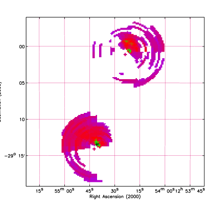
Figure 12: Residuals above $2$ in the X-ray brightness distribution. Given two regions, $A$ and $B$, of (length, width)${}=(2$ pixels$\approx 17$ arcsec$,30^{\circ})$ located symmetrically with respect to the center and with observed $C_{A}$ and $C_{B}$ counts respectively, the residuals are estimated as $\sigma=(C_{A}-C_{B})/\sqrt{C_{A}+C_{B}}$. An azimuthal scan with step of $30^{\circ}/3$ was done to smooth the map.

So far, we have adopted the working hypothesis, also supported from recent literature (e.g. Bardelli et al. 2001, Donnelly et al. 2001), that the two subclumps in A3528 are involved in a pre-merger along the North–South direction with zero impact parameter. This hypothesis fails, however, to explain the optical appearance and has remarkable difficulties to motivate the X-ray appearance of A3528, lacking any feature that characterize a merger between these two massive subclusters at a relative so small separation (and again, it is stringent the difference with the two clumps of Cygnus A which are separated by about 1 Mpc).

We consider here another explanation for what is observed, i.e. that the two subclumps are in an off-axis, post-merger phase. The X-ray emitting gas appears firmly confined in the central deep potential well of the two systems, giving rise to well defined gradients in surface brightness, temperature and metallicity profiles, whereas it seems more disturbed in the outskirts. As we show in Fig. 12, the surface brightness is azimuthally asymmetric with significant excesses in emission (with respect to the counter-part in opposition to the X-ray center) in the North–West region of A3528-N and in the North–East area of A3528-S. The latter X-ray excess coincides spatially with an enhancement in the optical light distribution. On the other hand, as we discuss in Section 4.1, no segregation in two clumps is observed in the galaxy distribution, being A3528-S marginally detectable (and the X-ray map confirms it as the most disturbed system). These results point toward a scenario in which the A3528-N and A3528-S are moving along the N-W/S-E and N-E/S-W direction, respectively, with a merger that had the closest encounter of the cores about 1–2 Gyrs ago with an impact parameter $b\approx 5r_{\rm s}$ and that was sufficient to disturb the outer galaxy distribution but not to affect the cluster cores themselves (Figure 4 in Ricker & Sarazin (2001) provides a reasonable representation of the kind of merger here suggested). We also note that this impact parameter is consistent with the observed separation between the clumps and the measured scale radius $r_{\rm s}$ in the NFW profile. Moreover, and following the results in Ricker & Sarazin (2001), this picture could explain the narrowness of the bridge connecting the two subclumps, whereas we should have expected a more extended emission in a head-on collision. Finally, the late stage of the merger and the non-zero impact parameter justify the absence of any detectable shock and, in particular, of a $M\sim 2$ case, estimated above from the calculated free-fall velocity, which holds only for head-on mergings (and this could be another point of difference in the comparison between A3528 and Cygnus A, where Markevitch and collaborators found good agreement between the velocities derived from the temperature jumps and the values predicted by free fall, corroborating the head-on merger hypothesis).

6 Summary

Using the high spatial resolution and large effective area of the EPIC instruments on board of XMM-Newton , we have performed a spatial analysis of the surface brightness, gas temperature and metal abundance distributions of the double cluster A3528 in the Shapley supercluster.

The main conclusions of our work are:

• the two clumps, A3528-N and A3528-S, have a mean gas temperature of $4.14\pm 0.09$ keV and $4.29\pm 0.07$ keV, respectively, that significantly decreases in the inner 30 arcsec (31 $h_{70}^{-1}$ kpc) to a deprojected value of $2.75^{+0.12}_{-0.20}$ keV and $3.06^{+0.10}_{-0.20}$ keV. The average estimate of the metal abundance in unit of the solar values from Grevesse & Sauval (1998) is $0.62\pm 0.05$ $Z_{\odot}$ in A3528-N and $0.45\pm 0.04$ $Z_{\odot}$ in A3528-S. A dramatic increase in metallicity is measured within 30$"$, with values of $1.79\pm 0.20$ ($2.16^{+0.23}_{-0.19}$ after deprojection) $Z_{\odot}$ in the Northern clump and $1.12\pm 0.11$ ($1.41^{+0.16}_{-0.15}$) $Z_{\odot}$ in the Southern clump. When rescaled to the set of abundances of Anders & Grevesse (1989), commonly used in the past literature, the metallicity in the core of A3528-N is 1.21 $Z_{\odot}$, a striking excess and together with the Centaurus cluster (Molendi et al. 2002; Sanders & Fabian 2002) the largest measured so far, exceeding the solar value. Their bolometric luminosities are $1.20\times 10^{44}\,\rm{erg\,s^{-1}}$ for A3528-N and $1.38\times 10^{44}\,\rm{erg\,s^{-1}}$ for A3528-S and they are consistent within the scatter observed in L-T relation for nearby systems (eg Fukazawa et al. 1998; Markevitch 1998)

• the presence in A3528-N and A3528-S of a centrally peaked surface brightness (see Fig. 2), a low temperature core and a steep positive gradient in metallicity moving inward (see Figs. 7, 8 and 9), with a cooling time that is about 10 per cent of the age of the Universe at $z=0.053$, suggests that they are in a relaxed state, despite their relative small separation (0.9 $h_{70}^{-1}$ Mpc as projected on the sky) and large masses ($\sim 1\times 10^{14}h_{70}^{-1}M_{\odot}$ at the virial radius) that should imply a strong merging action;

• an extended soft X-ray emission is detected between A3528-N and A3528-S, connecting the two clumps like a narrow bridge. We do not observe any evidence of shock heated gas, both in the surface brightness and in the temperature map. The surface brightness is not azimuthal symmetric, suggesting that A3528-N is falling from North–West to the South–East while A3528-S is moving from North–East to South–West. These facts, together with the optical light distribution more concentrated around A3528-N, indicate that an off-axis (with impact parameter of about $5r_{\rm s}$), post-merging (the closest cores encounter happened about 1–2 Gyrs ago) scenario is more plausible than a head-on pre-merger phase for the two subclumps.

Appendix A Details on the spectral analysis

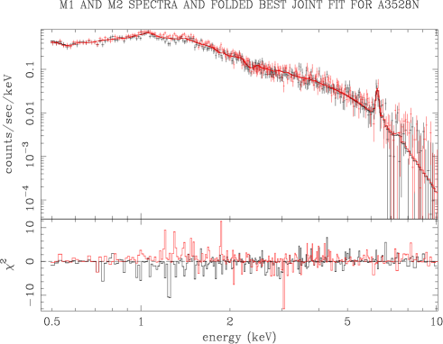
Figure 13: Joint fit of the two M1 (in black) and M2 (in red) spectra of A3528-N. Residuals are evident in the soft (0.5-2.0 keV) band.

Figure 14: MOS 1 data and folded model of the K iron line with free redshift and with fixed redshift at the optical value of 0.053 with the SASv5.3.3 in the upper panels and with SASv5.4.1 in the bottom panels.

In the spectral fitting done with the vignetting correction factor, we use the following response matrices: m1_medv9q20t5r6_all_15.rsp (MOS1), m2_medv9q20t5r6_all_15.rsp (MOS2) and, for PN, the set of ten single-pixel matrices (from epn_ff20_sY0_medium.rsp to epn_ff20_sY9_medium.rsp) depending on the mean of the values of “RAWY” of the photons collected in the region used to extract the spectrum. When the arf method is applied, we use m1_r6_all_15.rmf (MOS1), m2_r6_all_15.rmf (MOS2) and as before, depending on the mean “RAWY” of the region, the set of matrices from epn_ff20_sY0.rmf to epn_ff20_sY9.rmf for PN.

Bearing in mind that the observation was proposed to investigate in great detail the region between the two subclusters and the bulk of the emission of the two subclumps is 7 arcmin off-axis, where the quality of calibration is worse than for on-axis sources, we summarize here the main problems that emerged in the spectral analysis:

• there are differences between M1 and M2 at soft energies for A3528-N, resulting in very different $\rm{N_{H}}$ and different $\rm{kT}$ from the separate fits. This can be easily see in the residuals of the joint fit of the two cameras in Fig.13. The problem could be related to an incorrect modeling of the quantum efficiency of the two detectors (Lumb, private communication): the same problem emerges in the our re-analysis of the same regions in detector coordinates of M87 observation, performed with the thin filter.

• problems in the CTI/gain correction for MOS cameras, in particular the M1 where we see a clear discrepancy in the redshift determination which is different from the optical one. This could be due to the systematic drift to lower values (up to 20 eV at 6 keV) of the MOS line energies (Kirsch et al. 2002). If we fix the value of $\rm{N_{H}}\,$to the 21cm value and the redshift to the optical one, the M1 abundance is considerably lower ($0.54\pm 0.08$) due to the fact that it is impossible to fit correctly the iron K line which drives the abundance and redshift determination, as shown in the upper panels of Fig.14. This problem should be better addressed in the new version of the SAS, SASv5.4.1. We reprocessed the data but the problem is still open, although the line profile seems better determined, as shown in the bottom panel of Fig.14.

• differences between MOS and PN cameras, due to calibration uncertainties or to problems of background subtraction. It is known that PN camera shows a up to 15% higher flux than MOS from 0.5-1.5 keV, while for energies above 5 keV the MOS flux is up to 20% higher (Kirsch et al. 2002). But also a not correct background subtraction could result in different temperature determination.

For what concern the problems with the MOS1 camera, also our own analysis of the Perseus cluster, with superb statistics, gives systematically higher temperatures and abundances for MOS1 respect to MOS2 and PN. The conclusions of a recent work aimed at assessing the EPIC spectral calibration using a simultaneous XMM-Newton and BeppoSAX observation of 3C273 strengthen this fact: the MOS-PN cross calibration has been achieved to the available statistical level except for the MOS1 in the 3-10 keV band which returns flatter spectral slope (Molendi & Sembay 2003).

Appendix B Comparison of methods of vignetting correction

Table 1: Results of spectral fits on the two clusters for the three different cameras. PNS means that only single events (PATTERN==0) are considered. In the upper half we show the results obtained using the effective area files, while in the bottom half the results obtained performing the vignetting correction directly on the events.

	$\rm{N_{H}}$ ($10^{22}\,\rm{cm^{-2}}$)	kT (keV)	Z	z	$\rm{norm}^{a}$	$\chi^{2}$/d.o.f.
A3528 N M1	$0.0285^{+0.0059}_{-0.0062}$	$5.04^{+0.24}_{-0.22}$	$0.75^{+0.11}_{-0.10}$	$0.061^{+0.003}_{-0.002}$	$0.0115^{+0.0003}_{-0.0003}$	256/256
A3528 N M2	$0.0561^{+0.0060}_{-0.0057}$	$4.16^{+0.14}_{-0.15}$	$0.56^{+0.07}_{-0.07}$	$0.056^{+0.002}_{-0.002}$	$0.0138^{+0.0004}_{-0.0003}$	305/263
A3528 N PNS	$0.0361^{+0.0033}_{-0.0032}$	$4.22^{+0.10}_{-0.11}$	$0.59^{+0.06}_{-0.06}$	$0.052^{+0.002}_{-0.003}$	$0.0118^{+0.0003}_{-0.0003}$	587/525
A3528 S M1	$0.0500^{+0.0052}_{-0.0051}$	$4.52^{+0.13}_{-0.14}$	$0.43^{+0.06}_{-0.06}$	$0.055^{+0.002}_{-0.002}$	$0.0147^{+0.0003}_{-0.0003}$	304/301
A3528 S M2	$0.0502^{+0.0052}_{-0.0051}$	$4.25^{+0.13}_{-0.13}$	$0.39^{+0.06}_{-0.05}$	$0.062^{+0.002}_{-0.002}$	$0.0148^{+0.0003}_{-0.0003}$	299/296
A3528 S PNS	$0.0412^{+0.0030}_{-0.0037}$	$4.40^{+0.11}_{-0.10}$	$0.46^{+0.05}_{-0.05}$	$0.049^{+0.005}_{-0.005}$	$0.0139^{+0.0002}_{-0.0003}$	614/582

	$\rm{N_{H}}$ ($10^{22}\,\rm{cm^{-2}}$)	kT (keV)	Z	z	$\rm{norm}^{a}$	$\chi^{2}$/d.o.f.
A3528 N M1	$0.0317^{+0.0059}_{-0.0059}$	$4.79^{+0.24}_{-0.17}$	$0.70^{+0.11}_{-0.09}$	$0.062^{+0.003}_{-0.003}$	$0.0109^{+0.0003}_{-0.0003}$	341/337
A3528 N M2	$0.0581^{+0.0066}_{-0.0061}$	$4.05^{+0.15}_{-0.17}$	$0.57^{+0.08}_{-0.08}$	$0.056^{+0.003}_{-0.003}$	$0.0132^{+0.0004}_{-0.0004}$	404/344
A3528 N PNS	$0.0307^{+0.0032}_{-0.0034}$	$4.02^{+0.10}_{-0.11}$	$0.58^{+0.05}_{-0.06}$	$0.045^{+0.002}_{-0.004}$	$0.0109^{+0.0002}_{-0.0002}$	720/670
A3528 S M1	$0.0485^{+0.0054}_{-0.0050}$	$4.44^{+0.13}_{-0.15}$	$0.39^{+0.06}_{-0.06}$	$0.054^{+0.002}_{-0.002}$	$0.0141^{+0.0003}_{-0.0003}$	367/336
A3528 S M2	$0.0530^{+0.0052}_{-0.0052}$	$4.22^{+0.13}_{-0.13}$	$0.39^{+0.06}_{-0.06}$	$0.063^{+0.003}_{-0.003}$	$0.0138^{+0.0003}_{-0.0003}$	338/331
A3528 S PNS	$0.0414^{+0.0034}_{-0.0036}$	$4.23^{+0.12}_{-0.11}$	$0.44^{+0.05}_{-0.05}$	$0.049^{+0.003}_{-0.003}$	$0.0129^{+0.0002}_{-0.0002}$	770/671

^a The normalizations are quoted in units of $10^{-14}\,n_{e}\,n_{p}V/4\pi D_{A}(1+z)^{2}$ as done in XSPEC.

The reduction in effective area with radial distance from the field of view centre, an effect called vignetting, can seriously bias the brightness distribution and spectral modeling of extended sources as galaxy clusters. It is now customary in EPIC analysis of X-ray clusters to perform the vignetting correction directly to spectra, weighting each photon by the inverse of its vignetting, which is a function of off-axis angle and energy (vignetting is more severe for high energy photons). This approach is similar to the one used in the analysis of ROSAT PSPC data, corresponding to the CORRECT mode in EXSAS (Zimmermann et al. 1998). This method was proposed for XMM analysis of galaxy clusters by Arnaud et al. (2001) and opposed to the widely used method to compare the observed spectrum in a particular region of the detector with the incident source spectrum using an effective area (the ARF). This emission weighted effective area in the regions is derived from the observed global photon spatial distribution (see Davis 2001 for a formal derivation of the ARF in presence of an extended source). This is the main drawback because, apart from introducing extra noise, it biases the determination of spectral parameters. In fact the observed photon distribution is always more pronounced towards the center than the source distribution, so too much weight is given to central regions and the overall effective area is overestimated, and the overestimate is higher for higher energy photons. These kinds of biases are not introduced applying the correction directly to spectra because does not introduce any a priori assumptions about the spatial variation of the source.

As a partial overcome of the problems in the ARF method the ARF can be flux weighted using an image divided by an exposure map, in order to better represent the real source spatial distribution. This was done, following the recipe of Saxton & Siddiqui (2002), using exposure corrected images as detector maps (accumulated over square regions 1 arcmin on each side greater than the spectra extraction region) and with the parameter extended source of the SAS task arfgen switched to true (in order to avoid the PSF encircled energy correction). Obviously by dividing the image by a unique exposure map the real source spatial distribution is far from being recovered, because of systematic errors introduced by applying monochromatic exposure maps (as it is the case of the exposure maps created by the SAS task eexpmap, which assumes an energy which corresponds to the mean of the energy boundaries) to broad band images which encompasses a large range of variation in the effective area. These errors can be reduced if an exposure map is weighted according to the specific model of the incident spectrum (and this is easy for cluster spectra because a thermal spectrum with temperature the mean temperature of the cluster can be adopted). If the image contains significant spectral variation (as in cluster images, if they are relaxed because they have a cool core which can have a significantly lower temperature than the average of the cluster and if they are not relaxed because they can have significant temperature substructures) a single set of weights and thus a single exposure map cannot be applied to the entire image. Different exposure maps and different weights should be used for different parts of the image or the bandpass must be restricted to a range where the response is nearly flat (Houck 2001).

In this section as a first simple approach we compare the results obtained with the method of Arnaud (2001) and the ARF method using as a source distribution the image in the 0.5-8.0 keV band divided by a monochromatic exposure map with an energy of 4.25 keV (roughly according to the mean temperature of the two clusters). We fit the spectra of the two clumps with the two different methods and making no correction for the background and leaving all the parameters free, in order to take into account any possible difference arising. The results are shown in Tab.1 and we can see that the spectral parameters obtained by the two methods are consistent at the 1$\sigma$ level.

Appendix C Background subtraction

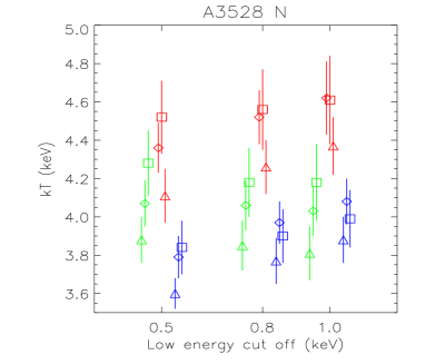
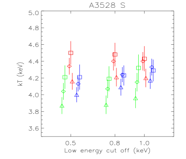
Figure 15: Measured temperature in function of different low energy cutoffs (the high energy cutoff is fixed at 8.0 keV because it had no effects on the measured temperature) for MOS1 (green), MOS2 (red) and PN singles (blue). Diamonds referred to fits with no background renormalization, triangles to fits with the renormalized background and squares to fits with the double subtraction. Uncertainties are at the 68% level for one interesting parameter ($\Delta\chi^{2}=1$).

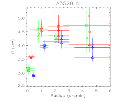
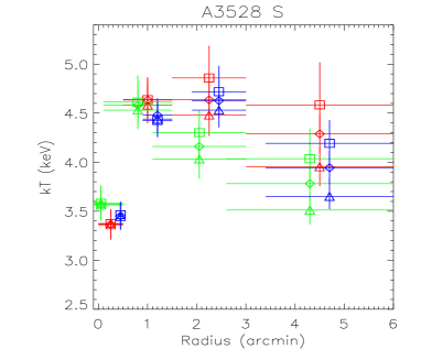
Figure 16: Same symbols as in Fig.15 for radial profiles.

For the detail of the double subtraction method we refer the reader to Appendix A of Arnaud et al. (2002). In this section we want to show how the different steps in the background subtraction affected the most sensitive of the spectral parameters, the temperature. In Fig.15 and in Fig.16 we see that the corrections go in the right way, in the sense that renormalizing the background at the level of the observation returns a lower temperature, while the further correction for the soft background returns a higher temperature. This correction is as we expect more crucial in the outer low surface brightness part of the cluster, as we see in the last radial bins of Fig.16, whether to indicate or not a temperature decline. A good test for the robustness of the temperature determination is to see its variation with the choosen energy band for fitting. The results for the subclumps are not much influenced by the fitting energy band.

References

- (1) Abell G.O., Corwin H.G., Olowin R.P., 1989, ApJSS, 70, 1
- (2) Anders E. & Grevesse N., Geochimica et Cosmochimica Acta, 53, 197
- (3) Arnaud K.A., 1996, ”Astronomical Data Analysis Software and Systems V”, eds. Jacoby G. and Barnes J., ASP Conf. Series vol. 101, 17
- (4) Arnaud M., Neumann D.M., Aghanim N., Gastaud R., Majerowicz S., Hughes J.P., 2001, A&A, 365, L80
- (5) Arnaud M., Majerowicz S., Lumb D., Neumann D., Aghanim N., Blanchard A., Boer M., Burke D., Collins C., Giard M., Nevalainen J., Nichol R.C., Romer K., Sadat R., 2002, A&A, 390, 27
- (6) Baldi A., Bardelli S., Zucca E., 2001. MNRAS, 324, 509
- (7) Bardelli S., Zucca E., Vettolani G., Zamorani G., Scaramella R., Collins C.A., MacGillivray H.T., 1994, MNRAS, 267, 665
- (8) Bardelli S., Pisani A., Ramella M., Zucca E., Zamorani G., 1998, MNRAS, 300, 589
- (9) Bardelli S., Zucca E., Zamorani G., Moscardini L., Scaramella R., 2000, MNRAS, 312, 540
- (10) Bardelli S., Zucca E., Baldi A., 2001, MNRAS, 320, 387
- (11) Binney J. & Tremaine S., 1987, Galactic Dynamics, Princeton University Press, p. 226f
- (12) Böhringer, H. & Schuecker P., 2002, in Merging Processes in Galaxy Clusters, Eds. Feretti L., Gioia I.M., Giovannini G., Astrophysics and Space Science Library, Kluwer Academic Plubishers, Vol. 272, p. 79
- (13) Buote D.A., 2002, in Merging Processes in Galaxy Clusters, eds. Feretti L., Gioia I.M., Giovannini G., Astrophysics and Space Science Library, Kluwer Academic Publishers, Vol. 272, p. 79
- (14) Cen R. & Ostriker J.P., 1994, ApJ, 429, 4
- (15) Colberg J.M., White S.D.M., Jenkins A., Pearce F.R., 1999, MNRAS,, 308, 593
- (16) Davis, J.E., 2001, ApJ, 548, 1010
- (17) Donnelly R.H., Forman W., Jones C., Quintana H., Ramirez A., Churazov E., Gilfanov M., 2001, ApJ, 562, 254
- (18) Ettori S., Fabian A.C., White D.A., 1997, MNRAS, 289, 787
- (19) Ettori S., Bardelli S., De Grandi S., Molendi S., Zamorani G., Zucca E., 2000, MNRAS, 318, 239
- (20) Ettori S., De Grandi S., Molendi S., 2002, A&A, 391, 841
- (21) Feretti L. & Venturi T., 2002, in Merging Processes in Galaxy Clusters, eds. Feretti L., Gioia I.M., Giovannini G., Astrophysics and Space Science Library, Kluwer Academic Publishers, Vol. 272, p. 163
- (22) Forman W., Jones C., Markevitch M., Vikhlinin A., Churazov E., 2002, in Merging Processes in Galaxy Clusters, eds. Feretti L., Gioia I.M., Giovannini G., Astrophysics and Space Science Library, Kluwer Academic Publishers, Vol. 272, p. 109
- (23) Fukazawa Y., Makishima K., Tamura T., Ezawa H., Xu H., Ikebe Y., Kikuchi K., Ohashi T., 1998, PASJ, 50, 187
- (24) Gastaldello, F. & Molendi, S., 2002, ApJ, 572, 160
- (25) Giovannini G. & Feretti L., 2002, in Merging Processes in Galaxy Clusters, eds. Feretti L., Gioia I.M., Giovannini G., Astrophysics and Space Science Library, Kluwer Academic Publishers, Vol. 272, p. 197
- (26) Girardi M. & Biviano A., 2002, in Merging Processes in Galaxy Clusters, eds. Feretti L., Gioia I.M., Giovannini G., Astrophysics and Space Science Library, Kluwer Academic Publishers, Vol. 272, p. 39
- (27) Grevesse N. & Sauval A.J., 1998, Space Science Reviews, 85, 161
- (28) Hanami H., Tsuru T., Shimasaku K., Yamauchi S., Ykebe Y., Koyama K., 1999, ApJ, 521, 90
- (29) Hasinger G., Schartel N., Komossa, S., 2002, ApJ, 573, L77
- (30) Henriksen M. & Jones C., 1996, ApJ, 465, 666
-
(31)
Houck J., 2001,
- (32) Kaastra J.S., 1992, An X-Ray Spectral Code for Optically Thin Plasmas (Internal SRON-Leiden Report, updated version 2.0)
- (33) Kirsch M. et al., “Status of the EPIC calibration and data analysis”, 2002, XMM-SOC-CAL-TN-0018
- (34) Landau L.D. & Lifshitz E.M, 1959, Fluid Mechanics, Publ. Pergamon Press, Oxford
- (35) Liedahl D.A., Osterheld A.L., Goldstein W.H., 1995, ApJ, 438, L115
- (36) Lumb D., 2002, XMM-SOC-CAL-TN-0016
- (37) Markevitch M. & Vikhlinin A., 1997, ApJ, 474, 84
- (38) Markevitch M, 1998, ApJ, 504, 27
- (39) Markevitch M., Sarazin C.L., Vikhlinin a., 1999, ApJ, 521, 526
- (40) Markevitch M., Gonzales A.H., David L., Vikhlinin A., Murray S., Forman W., Jones C., Tucker W., 2002, ApJL, 567, L27
- (41) Mewe R., Gronenschild E.H.B.M., van den Oord G.H.J., 1985, A&AS, 62, 197
- (42) Miller, N.A., Owen, F.N., 2003, AJ, 125, 2427
- (43) Molendi S., De Grandi S., Guainazzi M., 2002, A&A, 392, 13
- (44) Molendi S. & Sembay S., 2003, XMM-SOC-CAL-TN-0036
- (45) Navarro J.F., Frenk C.S., White S.D.M., 1997, ApJ, 490, 493
- (46) Raychaudhury S., Fabian A.C., Edge A.C., Jones C., Forman W., 1991, MNRAS, 248, 101
- (47) Reid A.D., Hunstead R.W., Pierre M.M., 1998, MNRAS, 296, 531
- (48) Ricker P.M. & Sarazin C.L., 2001, ApJ, 561, 621
- (49) Sanders J. & Fabian A.C., 2002, MNRAS, 331, 273
- (50) Sarazin C.L., 2002, in Merging Processes in Galaxy Clusters, eds. Feretti L., Gioia I.M., Giovannini G., Astrophysics and Space Science Library, Kluwer Academic Publishers, Vol. 272, p. 1
- (51) Saxton R.D. & Siddiqui H., 2002, XMM-SOC-PS-TN-43
- (52) Schindler S., 1996, MNRAS, 280, 309
- (53) Schindler S., 2002, in Merging Processes in Galaxy Clusters, eds. Feretti L., Gioia I.M., Giovannini G., Astrophysics and Space Science Library, Kluwer Academic Publishers, Vol. 272, p. 229
- (54) Shapley H., 1930, Harvard Obs. Bull., 874, 9
- (55) Snowden S.L., Egger R., Freyberg M.J., McCammon D., Plucinsky P.P., Sanders W.T., Schmitt J.H.M.M., Truemper J., Voges W., 1997, ApJ, 485, 125
- (56) Tormen G., Moscardini L., Yoshida N., MNRAS submitted, astro–ph/0304375
- (57) Venturi T., Bardelli S., Zambelli G., Morganti R., Hunstead R.W., 2001, MNRAS, 324, 1131
- (58) Venturi, T., Bardelli, S., Zagaria, M., Prandoni, I., Morganti, R., 2002, A&A, 385, 39
- (59) Vikhlinin A., Markevitch M., Murray S.S., 2001, ApJ, 551, 160
- (60) Yentis D.J., Cruddace R.J., Gursky H., Stuart B.V., Wallin J.F., MacGillivray H.T., Collins C.A. eds, Digitized Optical Sky Surveys, Kluwer, Dordrecht, p.67
- (61) Zimmermann U., Boese G., Becker W. et al., 1998, EXSAS User’s Guide MPE Report Rosat Scientific Data Center
- (62) Zucca E., Zamorani G., Scaramella R., Vettolani G., 1993, ApJ, 407, 470