The assembly of massive galaxies from NIR observations of the Hubble Deep Field South.

Abstract

We use a deep $K_{AB}\leq 25$ galaxy sample in the Hubble Deep Field South to trace the evolution of the cosmological stellar mass density from $z\simeq 0.5$ to $z\simeq 3$. We find clear evidence for a decrease of the average stellar mass density at high redshift, $2\leq z\leq 3.2$, that is $15^{+25}_{-5}\%$ of the local value, two times higher than what observed in the Hubble Deep Field North. To take into account for the selection effects, we define a homogeneous subsample of galaxies with $10^{10}M_{\odot}\leq M_{*}\leq 10^{11}M_{\odot}$: in this sample, the mass density at $z>2$ is $20^{+20}_{-5}\%$ of the local value. In the mass–limited subsample at $z>2$, the fraction of passively fading galaxies is at most 25%, although they can contribute up to about 40% of the stellar mass density. On the other hand, star–forming galaxies at $z>2$ form stars with an average specific rate at least $<\dot{M}/M_{*}>\simeq 4\times 10^{-10}$ yr^-1, 3 times higher than the $z\leq 1$ value. This implies that UV bright star–forming galaxies are substancial contributors to the rise of the stellar mass density with cosmic time. Although these results are globally consistent with $\Lambda$–CDM scenarios, the present rendition of semi analytic models fails to match the stellar mass density produced by more massive galaxies present at $z>2$.

1 Introduction

The most distintive features of current theories of galaxy formation is the mechanism relating the assembly of the galactic potential wells (mainly determined by the dark matter content) with the build-up of the stellar population contained therein. Hierarchical theories of galaxy formation are characterized by a gradual enrichment of the star content of galaxies driven by their progressive growth through merging events. In turn, this implies an appreciable antievolution with $z$ of the galacytic stellar mass distribution, in particular for the massive galaxies which, in hierarchical theories, have assembled relatively late.

Recent surveys have started to directly follow this process by estimating the stellar mass content of galaxies up to $z\sim 3$, either from detailed spectral analysis (Kauffmann et al 2002) or from multiwavelenght imaging observations (Giallongo et al 1998, Brinchmann and Ellis 2000, BE00 hereafter, Drory et al 2001, Cole et al 2001, Papovich et al 2001, P01 hereafter, Shapley et al 2001, Dickinson et al 2003, D03 hereafter). The latter technique relies on multicolor broad band imaging - extended into the near–IR range - to estimate the stellar content by a comparison with spectral synthesis models. In this work we present the results that this technique yields when applied to the Hubble Deep Field South (HDFS) data at $0<z<3.2$, and compare them with the predictions of a semi-analytic model in a $\Lambda$-dominated cosmology ($\Omega_{m}=0.3$, $\Omega_{\Lambda}=0.7$ and $H_{0}=70$ km s^-1Mpc^-1). A Salpter IMF is used in the paper.

2 Stellar masses from the HDFS data

The data that we use here are the results of the HDFS multiwavelength deep imaging survey, that combines the HST optical data (Casertano et al 2000) in the F300W, F450W, F606W and F814W filters (hereafter $U$,$B$,$V$ and $I$) and the ultradeep VLT-ISAAC IR images in the $Js$, $H$ and $Ks$ filters (the AB photometric system has been used throughout the paper). The latter data, that are in common with the FIRES survey (Labbe’ et al 2002, Franx et al. 2003), have typical exposure times of about 30 hr in each filter and were reduced and analyzed following the recipes described in Vanzella et al 2001 and Fontana et al 2000(F00 hereafter). An a posteriori correlation with the FIRES data shows a good agreement in the measured colors and noise estimates. We will use here the $K_{AB}\leq 25$ sample, where the $S/N$ ratio is larger than 5, although our results rely essentially on the brighter objects. The sample contains $302$ objects, $59$ of which with spectroscopic redshift (Vanzella et al. 2002 and Sawicki et al 2003), that were used to verify that the accuracy of photometric redshifts is comparable to our results in the HDFN.

On this catalog, we have estimated the stellar content of the HDFS galaxies by a comparison with spectral synthesis models, following the recepies of previous works (Giallongo et al. 1998, BE00, F00, P01, D03), In particular, we have adopted the same parametrization: we have used the Bruzual & Charlot (1993) GISSEL 2000 code with Salpter IMF, a range of exponentially declining star–formation histories with timescales from $\tau=0.1$ Gyrs to $\tau=\infty$ Gyrs, metallicities of $Z/Z_{\odot}=0.02,0.2,1,2.5$, and dust extinction ($0\leq E(B-V)\leq 1$). As in F00, we have also added a set of multiple burst models, although only 5% of the objects turned out to be fitted by such models. The best–fitting model to the observed multiwavelength distribution (at the spectroscopic or photometric redshifts) is used to estimate the stellar mass $M_{*}$ (which includes a correction for the recycled fraction) in each galaxy sample. As in P01, we tested both a SMC-like extinction curve (used as attenuation) and a Calzetti 2000 one. With the latter, the mass estimates are slightly smaller than SMC (25% on average), since the Calzetti curve yields lower fitted ages than the SMC, with an unpleasant fraction of 40% of galaxies wit ages $\leq$ 0.1 Gyrs at any $z$. The fits based on the Calzetti curve have also typically poorer $\chi^{2}$, and would be preferred only for 20%(40%) of the $z\leq 2$( $z>2$) galaxies. Given the uncertainities in the dust treatment, and due to these systematic differences, we present both results separately, with more emphasis on the SMC–based results.

The uncertainties involved in this approach, due to the degeneracy among the input models as well as from photometric noise and from the use of photometric redshifts, have been estimated on the basis of the reduced chi–square $\chi^{2}$, computed as in F00. The $1\sigma$ confidence levels on the fitted parameters (such as mass, age and star–formation rate) have been obtained by scanning the model grid and retaining only the models that have $\chi^{2}\leq\chi^{2}_{bestfit}+1$. Prior to this, as in P01, we have rescaled the noise in bright objects order to have $\chi^{2}_{bestfit}=1$ The scan is performed either at fixed redshift (for objects with known spectroscopic redshift) or allowing the models to move around the best–fitting photometric redshifts.

In the following, we shall also make use of a “Maximal Mass” estimate, to provide upper limits to the estimated stellar mass of each object, being still broadly consistent with the observed colors. We have first assumed that all the UV light is due to a recent starburst with minimal $M_{*}/L$ ratio (obtained from a model with constant SFR, $Z=0.2Z_{\odot}$, age$=0.2$Gyrs) and computed its contribution to the $K$ band flux. Then, we have used a maximally old stellar population to convert the residual $K$ band to $M_{*}$.

Finally we remind that, IR–selected samples do not strictly correspond to mass–selected ones. At any Hubble time (i.e. redshift), the faint side of the sample is biased against the detection of high–mass, low–luminosity objects, i.e. old, passively evolving or highly extincted galaxies. Because of the uncertainties in the modelling of such objects, it is difficult to define a clear selection threshold. We plot in Fig.1 two selection curves, such that objects above the lines should be used to compute statistics that require mass–selected samples, although several objects of lower mass (i.e. star–forming galaxies with lower $M_{*}/L$) are detected. In one case we use a GISSEL 2000 dust-free passively evolving model ignited by a histantaneous burst of sub–solar metallicity at $z=18$ (short-dashed line); in another we use the more realistic model of Le Borgne and Rocca–Volmerange 2002 (long-dashed line) that reproduces the colors of local E0 and that self–consistently includes the effects of finite burst duration, dust–absorption and metallicity evolution.

Our sample is definitely incomplete below these curves, and reasonably complete above, except for strongly obscured sources. In the following we will roughly adopt a completeness limit at $M=10^{10}M_{\odot}$ at $z>2$.

3 The galaxy stellar mass density

Fig. 1 shows the best–fit stellar mass derived for each galaxy in the HDFS, at the corresponding redshifts. We note that, due to the small volume sampled by the HDFS, the most massive objects have typical masses around $10^{11}M_{\odot}$ even at low–intermediate $z$, nearly a factor of ten smaller than those obtained by larger area surveys. We note however that several objects above $M_{*}\simeq 10^{10}M_{\odot}$ exist above $z=2$, the most massive being an ERO at $z_{phot}\simeq 2.8$ with $M_{*}\simeq 2\times 10^{11}M_{\odot}$, that is better described in a separate paper (Saracco et al. 2003).

To check whether the evolution of the more massive galaxies in our sample is consistent with theoretical expectations, we have used the CDM models of Menci et al. 2002 to compute a threshold $M^{*}_{th}$ defined such that one expects one galaxy above it (in the area sampled by the HDFS observations) per unit redshift (Fig.1, solid line). The curve follows the growth of the high–mass tail of the galaxy stellar mass function on a hierarchical scenario. Quantitavely, we find 17 galaxies above the threshold, against the expected 3, a first evidence that the high-mass tail of the galaxy stellar mass function is not adequately followed by present CDM models.

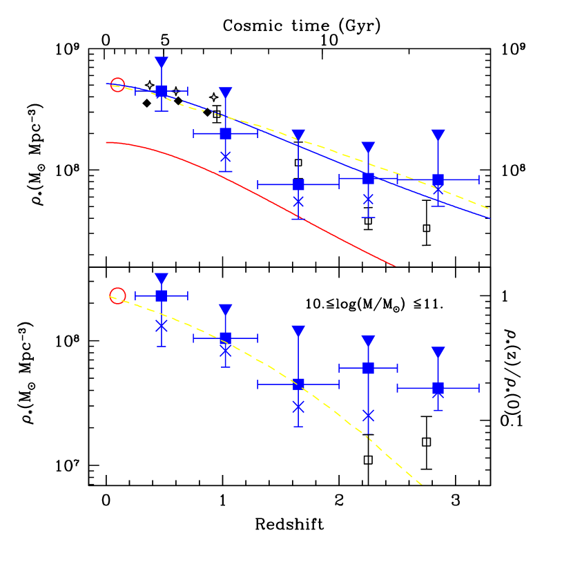
Figure 2: Evolution of the stellar mass density as a function of redshift. Upper panel: Observed values as estimated from the present work (solid squares, SMC; crosses, Calzetti) and from similar surveys: Dickinson et al 2003 (open squares), Cohen 2002 (open triangles), Brinchmann and Ellis 2000 (filled triangles), Cole et al 2001 (circle). Upper errorbar are extended at the level obtained from the “maximal mass” model, lower represent the number counts noise. The two solid lines are the results of integrating the cosmic star formation history, with and without dust (upper and lower curve, respectively). The dashed line is the result of the CDM hierarchical model of Menci et al 2002. Lower panel: Symbols and curves as in above, but computed only in the fixed mass interval $10^{10}M_{\odot}\leq M_{*}\leq 10^{11}M_{\odot}$.

In the upper panel of Fig.2, we present the stellar mass density $\rho_{*}(z)$ computed from our whole data sample with the standard $1/V_{max}$ estimator, corrected to account for incompleteness analogously to D03. We plot separately both the SMC and the Calzetti–based estimates. We also report in Fig.2 other available estimates of the stellar mass density as obtained from other surveys at $z\simeq 1$ (BE00, Cohen 2002), and most notably with the HDFN results (Dickinson et al. 2003), that has similar depth, size and adopted technique. While the evolution at $z\leq 1.5$ in both HDFs is consistent within errors (and with other surveys), it is remarkable to observe that we find in the HDFS a stellar mass density at $2\leq z\leq 3.2$ that is about two times higher than in HDFN.

At face value, the observed values of $\rho_{*}(z)$ witness a fast increase of the stellar mass density from 7-15% of the local (with an upper limit of 40%) at $z\geq 2$ to about unity at $z\leq 1$, i.e. in a relatively short amount of cosmic time. Following Cole et al. (2000) and D03 , we have compared the observed evolution with available theoretical expectations. We use an analytic fit to the global star–formation rate of Steidel et al. 1999, with two different dust extinctions ($E(B-V)=0,0.15$), and our CDM hierarchical model: both the CDM model and the integrated contribution of the global star–formation rate with a reasonable dust extinction provide a good fit to the data.

However, a clean interpretation of the HDFS data must take into account that the sampling of the underlying galaxy stellar mass function may be incomplete on the massive side, because of the small HDFS area, and may be inhomogenous at its faint side due to its varying depth as a function of $z$. For these reasons, we have also obtained a homogeneous estimate of its evolution computing the mass density only at $10^{10}M_{\odot}\leq M_{*}\leq 10^{11}M_{\odot}$ (Fig. 2, lower panel), where our sample is complete and well sampled at all $z$. This range is slightly below the typical Schecther mass in the local mass function of Cole et al. 2001. Similarly, we have also computed the same quantity in the HDF–N field, using the data of P01 and D03.

On this homogeneous subsample of relatively massive galaxies the stellar mass density at $z>2$ in the HDFS is $\simeq 20^{+20}_{-5}\%$ of the local value, and approaches the local one at $z\leq 1$. If we reproduce this selection criteria in our CDM model, that is overplotted in Fig.2, we find that the present CDM rendition dramatically fails to reproduce the stellar mass density in massive galaxies at $z\geq 2$. Again, we find that the HDF–N is underabundant of massive galaxies with respect to HDF–N, but is nevertheless well above the CDM predictions at $z\simeq 2.75$.

4 Star–forming and passive galaxies at $z>2$

We will analyze here the physical properties of the sample of $K\leq 25$ galaxies at $z_{phot}\geq 2$, that consists of 75 objects, including the 14 objects with $(J-K)_{AB}>1.34$ emphasized by Franx et al 2003.

First, we use the $J-K$ color to sample the amplitude of the rest–frame D4000 break, that is sensitive to the age of the stellar population We find that most of the $K$–selected $z\geq 2$ sample is distributed over a large range $0<(J-K)_{AB}\leq 1.5$, suggestive of a significant spread in the stellar population ages. This is confirmed by the ages obtained from the best–fit spectral templates, that are plotted as a function of $M_{*}$ in the upper panel of Fig.3. It is shown that the observed range of $J-K$ colors translates into a spread of fitted ages, ranging from $10^{8}$ to $3\times 10^{9}$ Gyrs for the complete $M_{*}\lower 2.15277pt\hbox{$\;\buildrel>\over{\sim}\;$}10^{10}M_{\odot}$ subsample, with about half of the sample close to the relevant Hubble time. At lower masses, the fraction of younger objects seems to increase, a result that is likely affected by the biases against old/passive low mass objects.

At the same time, we find that most of the sample is UV bright (see Poli et al 2003, Fig.2) and is restricted to the range of $0.1\lesssim V-I\lesssim 0.5$, corresponding to $0.05\lesssim E(B-V)\lesssim 0.2$ for an SMC extinction curve. We will use in the following the derived best–fit star formation rates (that include a correction for reddening), that are in agreement with those derived with a fixed conversion between the SFR and $L_{1400}$, assuming an $E(B-V)\simeq 0.15$.

Only seven “red” objects are detected at both large $V-I\lower 2.15277pt\hbox{$\;\buildrel>\over{\sim}\;$}1$ and $J-K\lower 2.15277pt\hbox{$\;\buildrel>\over{\sim}\;$}1.5$, a combination that may be due to either a strongly absorbed star–forming galaxy or to a passively fading stellar population, an ambiguity that cannot be safely removed without spectroscopy (Cimatti et al 2002). For the present dataset, we have found that the spectral fitting to the complete $UBVIJHK$ distribution slightly prefers the “passive” spectral model: when we force star–forming dusty solution by selecting $\tau/$age$\geq 2$, we find that typical $\chi^{2}_{red}$ are larger by a factor of 2, albeit being still statistically acceptables ($\chi^{2}_{red}\leq 1.4$).

The output of the fitting procedure is summarized in the lower panel of Fig.3, where we plot the specific star–formation rate $\dot{M}/M_{*}$ for the $K$–selected $z>2$ sample. At lower redshifts, the evolution of $\dot{M}/M_{*}$ has been studied by BE00, of which we plot in fig.3 their average relations at $0.2<z<0.5$ and at $0.75<z<1$. They showed evidence for an increase of the average $\dot{M}/M_{*}$ (at a given $M_{*}$) with $z$: we find that the trend of increasing $\dot{M}/M_{*}$ with $z$ still continues at $z\simeq 3$. A regression to our data yields $log(\dot{M}/M_{*})=2.18-1.245log(M_{*})$, i.e. the same slope but a factor 3 higher than the $z\simeq 1$ data. At the median value of the $M_{*}>10^{10}M_{\odot}$ complete sample ($M_{*}=3.2\times 10^{10}M_{\odot}$) the average specific star–formation rate as derived from the linear interpolation is $<\dot{M}/M_{*}>\simeq 4\times 10^{-10}$ yr^-1. We also note that the adoption of a Calzetti extinction curve would shift this it to a much higher value of $<\dot{M}/M_{*}>\simeq 2.3\times 10^{-9}$ yr^-1. We have found that the average Scalo $b$ parameter $SFR\times AGE/MASS$, as estimated from the best–fit quantites, is about 0.8 in this star–forming sample, suggesting a long duration of the starburst activity.

At the same time, we plot in Fig3 the seven “red” objects (over 30 of the mass–complete subsample) discussed before. These objects have $\dot{M}/M_{*}<10^{-10}$ yr^-1 i.e. more than 10 times lower that the typical $z\geq 2$ population if we adopt the “passively fading” fitting models, but follow the average trend if we adopt the “star–forming” solution. Given the ambiguity of their spectral classification, they can be used to obtain an upper limit to the fraction of galaxies that formed most of their stars in short episodes prior the time they are observed. In the HDF–S, these “passively fading” objects contribute at most to about 25% of the total number density of the mass–complete subsample of $z\simeq 3$ galaxies. In this case, the cosmologcal mass density due to these 7 objects is $1.95\times 10^{7}M_{\odot}$ Mpc^-3, and hence contributes up to $\simeq 40\%$ of the total mass density of the mass–complete subsample, that is of $4.5\times 10^{7}M_{\odot}$ Mpc^-3. As can be derived from Fig.3, the mass density does not change appreaciably if we assume the star–forming dusty solution for these objects.

Finally, we note that most of these “red” objects are drawn from the $(J-K)_{AB}>1.34$ subsample discussed by Franx et al. 2003, although other objects of this class are actively star–forming. The total mass density in the $(J-K)_{AB}>1.34$ sample is $3.7\times 10^{7}M_{\odot}$ Mpc^-3.

5 Summary

We have used new ultradeep $JHK$ images of the HDFS to trace the evolution of the stellar mass density $\rho_{*}(z)$ from $z\simeq 0.5$ to $z\simeq 3.5$, with the following main results:

- We find clear evidence for a decrease of the observed stellar mass density with increasing redshifts. At $2\leq z\leq 3.5$ the stellar mass density of both of the whole $K_{AB}\leq 25$ sample and of the homogeneous subsample of galaxies with $10^{10}M_{\odot}\leq M_{*}\leq 10^{11}M_{\odot}$ are about 15-20% (with a solid upper bound of 40%) of the local value, a value two times higher than the analogous result in the HDFN (Dickinson et al. 2003), and approaches the local value only at $z\simeq 1$. The UV–based cosmic star–formation history (e.g. Steidel et al 1999) reproduces the observed evolution of the total $\rho_{*}(z)$ (Fig.1).

- In the mass–limited subsample at $z>2$, we find that the fraction of passively fading galaxies is at most 25%, and they can contribute up to about 40% of the measured stellar mass density.

- Galaxies of $M_{*}\simeq 3\times 10^{10}M_{\odot}$ at $z>2$ form stars at a specific rate of at least $<\dot{M}/M_{*}>\simeq 4\times 10^{-10}$ yr^-1, a value 3 times higher than what observed at $z\leq 1$ (Brinchmann and Ellis 2000). The inverse of this rate is the time required for these objects to double their mass, assuming constant star–formation rate: in our sample, this turns out to be 2.5 Gyrs, comparable to both the Hubble time of the sample and to the cosmic time up to $z=1$. Given the high fraction of star–forming galaxies in our mass–complete sample at $z\simeq 2.5$, it is likely that their observed star–formation episodes last long enough to build up a substancial fraction of the observed mass density at $z\simeq 1$.

Overall, these data suggest a scenario where the growth of $\rho(z)$ in relatively massive galaxies is consistent with their UV–inferred star formation properties.

Finally, the large best fit ages and Scalo $b$ parameters of our $z>2$ galaxies suggest that the global star–formation rate should have been relatively high up to very high $z$, consistent with the results of recent searches of $z\simeq 5-6$ galaxies (e.g. Fontana et al 2003).

At first glance, this scenario is broadly consistent with the CDM theoretical expectation, where both “quiescent” star–formation rate and bursts during gas–rich mergings occurr at high rate at $z>1$. Despite this, our rendition of CDM models largely fails to reproduce the mass density of the most massive galaxies, even if we assume the average value between HDF–N and HDF–S. Hence, the dramatic failure to reproduce the amount of baryons condensed into stars suggests that the star–formation in these massive objects occurrs in a more efficient fashion than what accounted for by our recipes, as also suggested by other results directly related to the high star–formation rates found at $z\geq 3$ (Fontana et al. 2003, Poli et al. 2003).

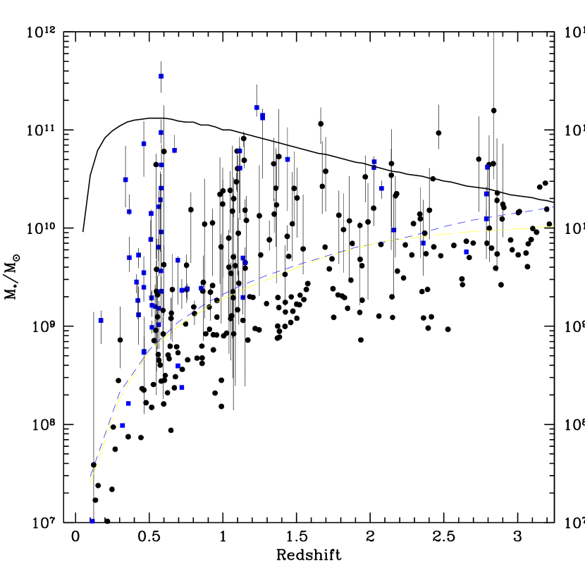
Figure 1: Galaxy stellar masses in the HDFS sample as a function of z. The points represent the “best–fit” estimates with SMC extinction curve of the stellar masses. Errorbars show the $1-\sigma$ confidence level and are computed including both the SMC and the Calzetti extinction laws. The solid line has been computed from the CDM hierarchical models of Menci et al 2002, such that about three objects are expected from $z=0$ to $z=3$. The short and long dashed line represent two possible selection curves above which the sample is mass–complete (see text for details).

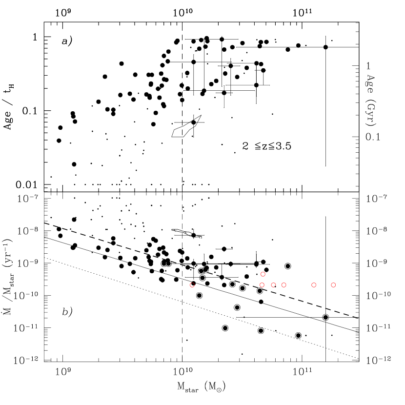
Figure 3: Rest frame properties of $z>2$ galaxies from spectral fitting of the HDFS sample. The vertical dashed line show the rough estimated limit for mass completeness in the $z>2$ sample. a) Best–fit age (divided by the corresponding Hubble time) as a function of stellar mass. For comparison, we show in the right vertical axis the corresponding ages at $z=2.5$. b) Specific star–formation rate as a function of stellar mass, compared with the average relations at $0.2<z<0.5$ (thin dotted line) and at $0.75<z<1$ (solid line) from Brinchmann and Ellis 2000. The thick dashed line correspond to our fit to the whole SMC sample. In both cases, filled dots represent the SMC-based estimates, small dots the Calzetti ones. Encircled points represent the objects with $J-K\geq 1.34$ discussed by Franx et al 2003. Errorbars are shown for a few objects, for the SMC case only: the large errorbars on the most massive objects reflect the ambiguity in its nature, between passively–fading and dusty–star forming objects. Note also that errors are typically correlated, as shown by the $1\sigma$ confidence regions shown for one of the objects. Empty points show the estimates of $\dot{M}/M_{*}$ when a star–forming dusty solution is forced for the objects with $\dot{M}/M_{*}\leq 10^{-10}yr^{-1}$: in this case the objects are fitted with slightly higher masses but without altering the order with respect to mass.

References

- (1) Brinchmann, J., Ellis, R.S., 2000, ApJ, 536, L77, BE00
- (2) Bruzual A., G., & Charlot, S., 1993, ApJ, 405, 538
- (3) Calzetti, D., Armus, L., et al. 2000, ApJ, 533, 68
- (4) Casertano, S., de Mello, D., et al., 2000, AJ, 120, 2747
- (5) Cimatti, A., Daddi, e., Mignoli, M. et al., 2002, A&A 381L 68
- (6) Cohen, 2002, ApJ, 567, 672
- (7) Cole, S., Norberg, P.; Baugh, C. M., et al., 2001, MNRAS, 326, 255
- (8) Dickinson, M., Papovich, C., Ferguson, H. C. & Budavari, T., 2003, ApJ, 587, 25 (D03)
- (9) Drory, N. et al., 2001, ApJL, 562, 111
- (10) Fontana,A.,D’Odorico,S.,Poli,F., et al., 2000, AJ, 120, 2206 (F00)
- (11) Fontana, A. et al., 2003, ApJ, 587, 544
- (12) Franx, M., Labbe’, I., Rudnick, G., et al., 2003, ApJ, 587, 25
- (13) Giallongo, E., D’Odorico, S., Fontana, A., et al, 1998, AJ 115, 2169
- (14) Kauffmann, G., Heckman, T. M., White, S. D. M. et al., 2002,
- (15) Labbe’ et al., 2003 AJ, 125, 1107
- (16) Le Borgne and Rocca Volmerange, 2002, A&A 386, 446
- (17) Menci, N., Cavaliere, A., Fontana, A., et al, 2002, ApJ, 575, 18
- (18) Papovich, C., Dickinson, M., Ferguson, H.C., 2001, ApJ, 559, 620 (P01)
- (19) Poli, F., et al., 2003, ApJL in press (astro-ph/0306625)
- (20) Saracco, P. et al 2003, A&A subm.
- (21) Sawicki, M., Mallen-Ornelas, G., 2003, AJ in the press (astro-ph/0305544)
- (22) Shapley, A.E., Steidel, C.C., Adelberger, et al., 2001, ApJ, 562, 95S
- (23) Steidel, C.C., et al., 1999, ApJ, 519, 1
- (24) Vanzella, E., Cristiani, S., Saracco, P., et al., 2001, AJ 122, 2190,
- (25) Vanzella, E., Cristiani, S., Arnouts, S., et al., 2002, A&A, 396, 847