A model for electromagnetic extraction of rotational energy
and formation of accretion-powered jets in radio galaxies

A self-similar solution for the 3D axi-symmetric radiative MHD equations, which revisits the formation and acceleration of accretion-powered jets in AGNs and microquasars, is presented. The model relies primarily on electromagnetic extraction of rotational energy from the disk plasma and forming a geometrically thin super-Keplerian layer between the disk and the overlying corona. The outflowing plasma in this layer is dissipative, two-temperature, virial-hot, advective and electron-proton dominated. The innermost part of the disk in this model is turbulent-free, sub-Keplerian rotating and advective-dominated. This part ceases to radiate as a standard disk, and most of the accretion energy is converted into magnetic and kinetic energies that go into powering the jet. The corresponding luminosities of these turbulent-truncated disks are discussed.
In the case of a spinning black hole accreting at low accretion rates, the Blandford-Znajek process is found to modify the total power of the jet, depending on the accretion rate.

1 Introduction

Recent theoretical and observational efforts to uncover the mechanisms underlying jet formation in AGNs and micro-quasars leave little doubt about their linkage to the accretion phenomena via disks Mirabel (2001); Livio (1999); Blandford (2001); Hujeirat et al. (2003).
The innermost part of a disk surrounding a black hole is most likely threaded by a large scale poloidal magnetic field (-PMF) of external origin Blandford & Payne (1982). Unlike standard accretion disks in which the sub-equipartition magnetic field (-MF) generates turbulence that is subsequently dissipated and radiated away, a strong PMF in excess of thermal equipartition may suppress the generation of turbulence and acts mainly to convert the shear energy into magnetic energy. A part of the shear-generated toroidal magnetic field (-TMF) undergoes magnetic reconnection in the launching layer, whereas the other part is advected outwards to form relativistic outflows Hujeirat et al. (2003).
Indeed, the total power of the jet in M87 is approximately $L_{\mathrm{J}}\approx 10^{44}\,erg\,s^{-1}$ Bicknill & Begelman (1999). This is of the same order as the power resulting from a disk accreting at the rate ${\,\dot{\cal M}}\approx 1.6\times 10^{-3}{\,\dot{\cal M}}_{\mathrm{Edd}}$ Di Matteo et a. (2003). Similarly, the variabilities associated with the microquasar GRS 1915-105, as have been classified by Belloni et al. (2000), consists of a state ”C” which corresponds to the case when the innermost part of the disk diminish Fender (1999), probably a phase in which the super-luminal jet is fed with rotational and magnetic energies.
Another two additional basic questions related to jet formation are: 1) What are the contents of these jets? specifically, are they made of electron-positron $(e^{-}/e^{+})$, electron-proton $(e^{-}/p)$ or a mixture of both. 2) How significant is the role of the central object in the formation and acceleration of jet-plasmas?
It is generally accepted that electron temperature $\vartheta_{\mathrm{e}}(\,=kT/m_{\mathrm{e}}c^{2})$ of order unity can be easily achieved in accretion flows onto BHs, and specifically in the vicinity of the event horizon. At such high temperatures pair creation becomes possible. The efficiency of pair creation depends mainly on the interplay between the optical depth to scattering $\tau_{\mathrm{p}}=\rho\kappa_{\mathrm{sc}}H$, on the so called ”compactness” parameter $\ell=\alpha_{0}q^{-}H^{2}$ and on the strength of the magnetic field Björnsson & Svensson (1991); Esin (1999). H here denotes the thickness of the disk or a relevant length scale, $\alpha_{0}$ is a constant coefficient, $\rho$ is the density and $\kappa_{\mathrm{sc}}$ is the opacity due Thomson scattering, and $q^{-}$ is the radiative emissivity. Generally, the efficiency of pair creation decreases strongly with increasing the optical depth $\tau_{\mathrm{p}}$. It decreases also if the strength of the magnetic field is increased. Esin (1999) has studied pair creation in steady hot two-temperature accretion flows for a large variety of parameters. The ions here are preferentially heated by turbulent dissipation and cool via Coulomb interaction with the electrons, which in turn are subject to various cooling processes such as Bremsstrahlung and Synchrotron emission. Esin (1999) showed that two-temperature accretion flows are almost pair-free, whereas single-temperature accretion flows are more appropriate for pair-dominated plasmas. However, enhancing thermal coupling between electrons and protons, or heating electrons and protons at an equal rate, and relaxing the stationarity condition may lead to $e^{-}/e^{+}$-dominated plasma, provided the accretion rate is sufficiently low.
In the case the BH is rotating and accreting at low rates, formation of $e^{-}/e^{+}$ jets though electromagnetic extraction of rotational energy from the hole via Blandford-Znajek (1977) process is very likely Rees et al. (1982). Indeed, recent observations reveals that the jet-plasma in M87 is probably an $e^{-}/e^{+}-$dominated jet Reynolds et al. (1996). Furthermore, Wardle et al. (1998) reported about the detection of circularly polarized radio emission from the jet in the quasar 3C 279. The circular polarization produced by Faraday conversion requires the radiative energy distribution to extend down to low energy bands, which indicate that $e^{-}/e^{+}-$ plasma population might be a significant fraction of the jet-contents.
On the other hand, recently it has been argued that unless the poloidal magnetic field threading the event horizon is exceptionally strong, the total available power through the Blandford-Znajek process is dominated by the accretion power of the the disk Ghosh & Abramowicz (1997); Livio et al. (1999). We note, however, that the PMF can be sufficiently strong, if the innermost part of the disk collapses dynamically, while conserving poloidal magnetic flux Hujeirat et al. (2003), and which may significantly enhance the efficiency of the Blandford-Znajek process.
In this paper we present a theoretical model for the formation of accretion-powered jets in AGNs and microquasars. The model relies mainly on electromagnetic extraction of rotational energy from the disk plasma and deposit it into a geometrically thin layer between the disk and the overlying corona (Sec. 3). In Section 4 we discuss the content of the plasma in the TL. The role of the Blandford-Znajek process in combination with the luminosity available from the transition layer is discussed is discussed in Sec. 5. We compute the total luminosity of truncated disks in Sec. 6, and end up with summary and conclusions in Section 7.

Figure 1: A schematic illustration of the jet-disk connection model. In the outer disk, $r\geq r_{\mathrm{tr}}$, MFs are weak and advected around by fluid motions. Balbus-Hawley and Parker-instabilities in combination with reconnection and fast inwards fluid-motions amplify the MFs and reach thermal equipartition at $r_{\mathrm{tr}}$. Interior to $r_{\mathrm{tr}}$, MFs become of large scale topology relative to the flow in the disk, hence adopting the profile $r^{-2}$ to conserve the poloidal magnetic flux. Here, torsional $\rm Alfv\acute{e}n$ waves are the dominant angular momentum carrier. They transport angular momentum from the disk upwards and form a super-Keplerian thin layer, where the plasma rotates super-Keplerian, virial-heated by reconnection, and start to centrifugal-accelerate outwards.

2 The model problem

Let $r=r_{\mathrm{tr}}$ be a transition radius, where the effects of magnetic fields on the dynamics of accretion flows become significant. This may occur if the initially weak magnetic fields in the dissipative-dominated disk-plasma are amplified via dynamo action, in which Balbus-Hawley (1991) instability in combination with the Parker instability results in a topological change of the magnetic field from a locally disordered into well-ordered large scale magnetic field (see Fig. 1). At this radius the MFs are in equipartition with the thermal energy of the plasma, i.e., $\beta=E_{\mathrm{mag}}/E_{\mathrm{th}}=1.$

Interior to $r_{\mathrm{tr}}$ the poloidal magnetic field $B_{\mathrm{p}}$ is predominantly of large scale, and magnetic flux conservation implies that PMF increases inwards obeying the power law $B_{\mathrm{p}}\sim r^{-2}.$ Such a strong PMF suppresses the generation of turbulence, whenever $\beta$ exceeds unity. In this case, the heating mechanisms that hold the plasma against runaway cooling are magnetic reconnection, adiabatic compression and other non-local sources such as radiative reflection, Comptonization and conduction of heat flux from the surrounding hot media.
Given a plasma threaded by an $r^{-2}-$ PMF, the angular velocity must deviate significantly from its corresponding Keplerian profile. This is because torsional $\rm Alfv\acute{e}n$ waves (-TAWs) extract rotational energy from the disk plasma on the time scale: $\tau_{\mathrm{TAW}}=H_{\mathrm{d}}/V^{\mathrm{P}}_{\mathrm{A}},$ which decreases strongly inwards. $V^{\mathrm{P}}_{\mathrm{A}}$ here is the $\rm Alfv\acute{e}n$ speed due to the PMF. The TAW crossing time of the disk, i.e., $\tau_{\mathrm{TAW}}$, is of the same order, or it can be even shorter than the dynamical time scale $\tau_{\mathrm{dyn}}=r/V_{\mathrm{\varphi}}$. In this case the angular velocity becomes sub-Keplerian, and the disk becomes pre-dominantly advection-dominated. If $\tau_{\mathrm{TAW}}<\tau_{\mathrm{dyn}},$ accretion may terminate completely.
TAWs, which carry with it rotational energy from the disk-plasma, may succeed to propagate through the overlying corona without being dissipated. This corresponds to magnetic braking of the disk, in which the rotational energy is transported from the disk and deposited into the far ISM. However, since the PMF-lines rotate faster as the equator is approached, the PMF winds up, intersect and subsequently reconnect, and so inevitably terminate the propagation of TAW into higher latitudes. Alternatively, the vertical propagation of the TWAs may terminate via magnetic reconnection at the surface of the disk, establishing thereby a highly dissipative transition layer (TL), i.e., chromosphere, where the toroidal magnetic fields intersect, reconnect and subsequently heat and particle-accelerate the plasma in the TL. The latter possibility is more plausible, mainly because:

1. The vertical profile of the angular velocity generate a toroidal magnetic field of opposite signs, i.e., anti-parallel toroidal flux tubes, which give rise to magnetic reconnection of the toroidal magnetic field lines (-TMF). The reconnection process terminates the vertical propagation of the TAWs, inducing thereby a magnetic trapping of the rotational energy in the TL. As a consequence, a centrifugally induced outflow is initiated, which carries with it rotational, thermal and magnetic energies.

2. Unlike stellar coronae that are heated from below, BH-coronae have been found to be dynamically unstable to heat conduction Hujeirat et al. (2002). The effect of conduction is to transport heat from the innermost hot layers into the outer cool envelopes. Furthermore, noting that the Lorenz and centrifugal forces in an axi-symmetric flow attain minimum in the vicinity of the rotational axis, we conclude that this region is inappropriate for initiating outflows.

3. In a stable flow-configuration, an isolated Keplerian-rotating particles in the disk region move along trajectories with minimum total energy. If these particles are forced to move to higher latitudes while conserving their angular momentum, then their rotation velocity becomes super-Keplerian, and therefore start to accelerate outwards as they emerge from the disk surface. Since the speed of these motions and the associated strength of the generated toroidal flux tubes increase inwards, the magnetic flux tubes are likely to interact and subsequently to reconnect.

4. Observations reveals that the radio luminosity in the vicinity of the nucleus of various AGNs with jets acquire a significant fraction of the total luminosity. This indicates the necessity for an efficient heating mechanism that allow the electrons to continuously emit Synchrotron radiation on the $\rm Alfv\acute{e}n$ wave crossing time. Noting that $B_{\mathrm{p}}\sim r^{-2}$, and that the plasma in the innermost part of the disk is turbulent-free, we propose that magnetic reconnection of the TMF is most reasonable mechanism for heating the plasma in the TL. This agrees with the proposal of Ogilvie & Livio (2001) who argued that jet launching requires thermal assistance.

2.1 The velocity field

The problem we are addressing in this paper is: assume that the innermost part of the disk is threaded by $r^{-2}-$ PMF. What are the most reasonable power-law distributions of the other variables in both, the disk and in the TL, that give rise to inflow-outflow configuration, and which simultaneously satisfies the set of the steady 3D axi-symmetric radiative MHD equations. As we shall see in the next sections, there are several signatures that hint to $\Omega\sim r^{-5/4}$ as the optimal profile (see Fig. 2). Nevertheless, we will consider this profile as an assumption.
Therefore, in the disk region the following profiles are assumed:

$$\Omega(r)=\Omega_{0}X^{-5/4},\,B_{\mathrm{p}}(r)=B_{\mathrm{\theta}}(r)\approx B_{0}X^{-2},$$ (1)

where $X=r/r_{\mathrm{tr}}$.
To assure a smooth matching of the variables interior to $r_{\mathrm{tr}}$ with those of the standard disk exterior to $r_{\mathrm{tr}}$, we set $\Omega^{2}_{0}=GM/{r_{\mathrm{tr}}^{3}}$, and ${B_{0}^{2}}={B^{2}}(r=r_{\mathrm{tr}})=(12\pi{\cal{R}_{\mathrm{g}}}/\mu(\gamma-1))\rho T|_{r=r_{\mathrm{tr}}}$, Inserting $\Omega(r)$ in Equation A.2 (see Appendix), and taking into account that the internal and magnetic energies of the plasma at $r_{\mathrm{tr}}$ are negligibly small compared to the gravitational energy of the flow, the radial velocity then reads:

$$U_{\mathrm{d}}(r)=[U^{2}_{0}+\frac{2}{\epsilon^{2}}\frac{1}{r_{\mathrm{tr}}}(\frac{1}{X}-1)]^{1/2}.$$ (2)

As in classical disks, we set $U_{0}=U(r=r_{\mathrm{tr}})=-(2/3)\nu/r_{\mathrm{tr}}$, and $\nu=\alpha_{\mathrm{ss}}H_{\mathrm{d}}V_{\mathrm{s}}$ for describing turbulent viscosity.

Figure 2: The profiles of the angular velocity in the innermost part of the disk and in the launching region. TAWs extract rotational energy from the disk-plasma efficiently and deposit it into the plasma adjusting to the disk-surface. As a consequence, the inflow adopts the sub-Keplerian profile $\Omega\sim r^{-5/4}$ in the disk-region, while the outflow adopts the super-Keplerian profile $\Omega\sim r^{-5/4}$ in the TL. Note that the up-stream boundary conditions determine whether the flow is sub- or super-Keplerian rotating.

The radial accretion rate in the disk region is obtained by $\theta-$integrating the continuity (Eq. A.1):

$$\frac{\partial}{\partial r}{\,\dot{\cal M}}^{\mathrm{d}}_{\mathrm{r}}=2r\cos{\theta_{\mathrm{d}}}(\rho V)|_{\theta_{\mathrm{d}}},$$ (3)

where ${\,\dot{\cal M}}_{\mathrm{d}}^{\mathrm{r}}=r\Sigma_{\mathrm{d}}U_{\mathrm{d}}$ is the radial accretion rate in the disk region, and $\Sigma_{\mathrm{d}}=\int^{\theta_{\mathrm{d}}}_{-\theta_{\mathrm{d}}}{r\cos{\theta}\rho_{\mathrm{d}}d\theta}$. $\theta_{\mathrm{d}}$ is the angle such that $\tan{\theta_{\mathrm{d}}}=H_{\mathrm{d}}/r,$ where $H_{\mathrm{d}}$ is the vertical scale height of the disk (see Fig. 3).

Furthermore, it is reasonable to assume that the radial dependence of the density at the surface of the disk does not differ significantly from the density at the equator. Thus, $\rho(r,\theta=\theta_{\mathrm{d}})/\rho(r,\theta=0)=const.<<1$.

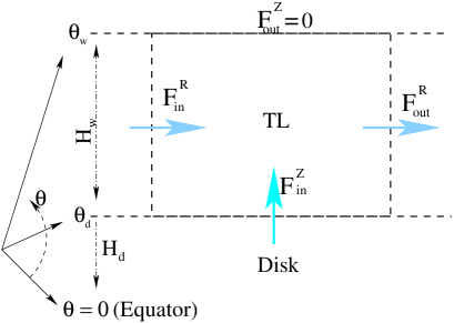
Figure 3: The material fluxes governing an arbitrary volume cell in the TL are shown. $\theta_{\mathrm{W,d}}$ are latitudes that correspond to the locations of the interface between the disk and the TL, and to the upper surface of the TL, respectively. ${\rm F}^{\mathrm{Z}}_{\mathrm{in,out}}$ and ${\rm F}^{\mathrm{R}}_{\mathrm{in,out}}$ denote the material fluxes across the vertical and radial surfaces. The width of the cell is $H_{\mathrm{W}}$, and the vertical material flux across $\theta_{\mathrm{W}}$ is set to vanish.

Similar to the disk region, the following angular velocity and the PMF profiles are set to govern the plasma in the launching region:

$$\Omega(Y)=\Omega^{\mathrm{W}}_{0}Y^{-5/4},\,B_{\mathrm{p}}(Y)\approx B_{\mathrm{r}}=B^{\mathrm{W}}_{0}Y^{-2},$$ (4)

where $Y=r/r_{\mathrm{BL}}$, and $r_{\mathrm{BL}}$ is the innermost radius of the TL, where the effective gravity is set to vanish. This implies that at $Y=1$, the angular velocity approaches the Keplerian values: $\Omega^{\mathrm{W}}_{0}=\Omega^{\mathrm{W}}(Y=1)=\sqrt{GM/{r_{\mathrm{BL}}^{3}}}$. Inspection of Eq. A.2 implies that the radial velocity in the super-Keplerian region has the profile:

$$U_{\mathrm{W}}(Y)=[U^{2}_{\mathrm{W,0}}+\frac{2}{\epsilon^{2}}\frac{1}{\sqrt{r_{\mathrm{tr}}}}(1-\frac{1}{\sqrt{Y}}]^{1/2}.$$ (5)

where $U_{\mathrm{W,0}}$ is the radial velocity at $r_{\mathrm{BL}}$. However, since the effective gravity has a saddle point at $r_{\mathrm{BL}}$, the radial velocity must vanish. Interior to $Y=1$, the plasma is gravitationally bound, so that the plasma and the associated rotational energy will be advected inwards and disappear in the hole. In the case of a spinning BH, $r_{\mathrm{BL}}$ is likely to be located inside the ergosphere.
The outward-oriented material flux in the TL is:

$${\,\dot{\cal M}}^{\mathrm{W}}_{\mathrm{r}}=r\Sigma^{\mathrm{W}}U^{\mathrm{W}},$$ (6)

where $\Sigma^{\mathrm{W}}=\int^{\theta_{\mathrm{W}}}_{\theta_{\mathrm{d}}}{r\cos{\theta}\rho^{\mathrm{W}}d\theta}$. $\theta_{\mathrm{W}}$ is the angle such that $\tan{\theta_{\mathrm{W}}}-\tan{\theta_{\mathrm{d}}}=H_{\mathrm{W}}/r,$ and $H_{\mathrm{W}}$ is the vertical scale height of the launching layer.
Global mass conservation of the plasma both in the disk and in TL regions requires that:

$$\frac{\partial}{\partial r}{\,\dot{\cal M}}^{\mathrm{d}}_{\mathrm{r}}=2\frac{\partial}{\partial r}{\,\dot{\cal M}}^{\mathrm{W}}_{\mathrm{r}},$$ (7)

where mass loss from both sides of the disk has been taken into account, and where have assumed a vanishing vertical flux of matter across $\theta_{\mathrm{W}}$ (see Fig. 2 ).

2.2 The geometrical thickness of the launching region

Since the plasma in the TL rotates super-Keplerian, the horizontal component of the centrifugal force, i.e., $({\tan{\theta}}/{\epsilon^{2}})({V_{\mathrm{\varphi}}^{2}}/{r})$ (see Eq. A.3), acts to compress the plasma in the launching region toward the equator and its collapse. Inspection of Eq. A.3 reveals that there are four forces that may oppose collapse: gas and turbulent pressures, poloidal and toroidal magnetic fields. In terms of Eq. A.3, the dominant terms required for establishing such an equilibria are:

$$\frac{\tan{\theta}}{\epsilon^{2}}\frac{V_{\mathrm{\varphi}}^{2}}{r}=\left\{\begin{array}[]{lcl}\frac{1}{\rho}\frac{1}{r}\frac{\partial}{\partial\theta}P_{\mathrm{gas}}:&&{\rm ion\,pressure}\,\,(I)\\ \frac{1}{\rho}\frac{1}{r}\frac{\partial}{\partial\theta}P_{\mathrm{tur}}:&&{\rm turbulent\,pressure}\,\,(II)\\ \frac{1}{\rho}\frac{1}{r}\frac{\partial}{\partial\theta}B_{\mathrm{p}}^{2}:&&{\rm poloidal\,MFs}\,\,(III)\\ \frac{1}{\rho}\frac{1}{r}\frac{\partial}{\partial\theta}B_{\mathrm{T}}^{2}:&&{\rm toroidal\,MFs}\,\,(IV).\end{array}\right.$$ (8)

Equivalently, the relative geometrical thickness of the TL reads:

$$\frac{H_{\mathrm{W}}}{r}=\left\{\begin{array}[]{lcl}\epsilon\times({V_{\mathrm{S}}}/{V_{\mathrm{\varphi}}}):&&\,\rm{ion\,pressure}\,\,(I)\\ \epsilon\times({V_{\mathrm{tur}}}/{V_{\mathrm{\varphi}}}):&&\,\rm{turbulent\,pressure}\,\,(II)\\ \epsilon\times({V^{\mathrm{P}}_{\mathrm{A}}}/{V_{\mathrm{\varphi}}}):&&\,\rm{poloidal\,MFs}\,\,(III)\\ \epsilon\times({V^{\mathrm{T}}_{\mathrm{A}}}/{V_{\mathrm{\varphi}}}):&&\,\rm{toroidal,MFs}\,\,(IV),\end{array}\right.$$ (9)

were we have excluded magnetic tension from our consideration, because the plasma in the TL is dissipative. Global magnetic flux conservation, i.e., $\nabla\cdot B=0$, requires that $B_{\mathrm{p}}$ must bend as it emerges from the disk region, provided that $B_{\mathrm{p}}$ is of large scale topology and is advected inwards with the matter. In this case, the above-mentioned third possibility, i.e., case III, applies to those MFs in which $B_{\mathrm{r}}$ decreases vertically and therefore may hold the plasma in the TL against vertical collapse. This means that the MF-lines in the TL must point toward the central BH as they emerge from the disk (see Fig. 4). Although such configurations are not in view with our classical expectation about magnetic-induced launching, the radiative MHD calculations do not appear to exclude such solutions, provided that TL-plasma is highly dissipative. On the other hand, if the poloidal MF-lines in the TL point away as they emerge from the disk, which is the case we are considering in this study, $B_{\mathrm{r}}$ must increase in the vertical direction, and therefore may enhance the collapse. Therefore, taking into account that the electron thermal energy and the PMF-energy are relatively small compared to the rotational energy in the super-Keplerian layer, and that $B_{\mathrm{T}}-$profile has turning points in the TL, we may conclude that $P_{\mathrm{tur}}$ is the most reasonable force to oppose the TL-collapse.
To elaborate this point we note that when TAWs start propagating from the disk upwards while carrying angular momentum, a profile such as shown in Fig. 5 would result. This profile has $\nabla\Omega$ of mixed signs, which therefore induces the formation of toroidal flux tubes whose the associated electric currents $\@vec{j}$ move anti-parallel around the axis of rotation, and which gives rise to partial magnetic reconnection (Fig. 5).
The strong shear in the TL is capable to produce magnetic energy that is in equipartition with the rotational energy, i.e., $V^{\mathrm{T}}_{\mathrm{A}}\approx V_{\mathrm{\varphi}}$, which is necessary to maintain the steadiness stationarity of the solution of the $B_{\mathrm{T}}-V_{\mathrm{\varphi}}$ coupled system.
We note that magnetic reconnection is a common phenomena in astrophysical MHD-flows, which is generally associated with changes in the magnetic field topology and partial loss of the magnetic flux. In the solar case, for example, magnetic reconnection is one of the main mechanisms underlying the eruption phenomena of the solar flares. Approximately $10^{32}$ ergs are liberated in each event and on the time scale of few minutes. Although the sun is not as compact as old stars such as a white dwarf or a neutron star, solar flares appear to be associated with $\gamma-$ray emission, electron-positron annihilation at 511 Kev, and most impressively, with the neutron capture by the hydrogen nucleus which occurs at about two mega electron volts, revealing thereby that acceleration of particles up to relativistic velocities is an important ingredient of the reconnection process.
Yet, the TL is located deep in the gravitational well of the central BH, and if reconnection occurs, then the energetics associated must be much powerful than in the solar flares, and a significant populations of $e^{-}/e^{+}$ are to be expected in the TL.
In plasma physics, reconnection occurs normally on microscopic scales. In the present study we assume that reconnection can be described by the magnetic diffusivity:

$$\nu_{\mathrm{mag}}=H_{\mathrm{W}}V_{\mathrm{tur}},$$ (10)

where $H_{\mathrm{W}}$ is the width of the TL and $V_{\mathrm{tur}}$ is the velocity that is associated with magnetic reconnection. We adopt the Petscheck-scenario for describing the the reconnection velocity Priest (1994):

$$V_{\mathrm{rec}}=V_{\mathrm{tur}}=\alpha_{\mathrm{mag}}V^{\mathrm{T}}_{\mathrm{A}}/\log{Re},$$ (11)

where $\alpha_{\mathrm{mag}}$ is a constant less than unity and $\log(Re)$ is the logarithm of the magnetic Reynolds number.
Inserting $V_{\mathrm{tur}}=\alpha_{\mathrm{mag}}V^{\mathrm{T}}_{\mathrm{A}}/\log(Re)$ in Eq. 9/II, we obtain:

$$\frac{H_{\mathrm{W}}}{r}=\frac{V_{\mathrm{tur}}}{V_{\mathrm{\varphi}}}=\frac{\alpha_{\mathrm{mag}}}{\log(Re)}$$ (12)

From the definition of the magnetic Reynolds number:

$$Re=\frac{\rm{Inertial\,force}}{\rm{Viscous\,force}}=(\frac{Bp}{B_{\mathrm{T}}})(\frac{V_{\mathrm{\varphi}}}{V_{\mathrm{tur}}})=(\frac{Bp}{B_{\mathrm{T}}})(\frac{\log{Re}}{\alpha_{\mathrm{mag}}}),$$ (13)

we obtain an equation for the magnetic Reynolds number:

$$\log(Re)-[\alpha_{\mathrm{mag}}(\frac{B_{\mathrm{T}}}{B_{\mathrm{p}}})]Re=0.$$ (14)

Obviously, $\alpha_{\mathrm{mag}}$ must be relatively small for this equation to provide a positive $Re$ (see Fig. 6), which means that the TL must be geometrically thin, and that $\epsilon\approx\alpha_{\mathrm{mag}}/\log{Re}=H_{\mathrm{W}}/r$. In order to assure that the outflow leaving the system has sufficient TMF to collimate and reach large Lorentz factors, we require that only a small fraction of the total generated TMF dissipate in the TL through reconnection events, while the rest is advected outwards. Therefore, the advection time scale should be equal to the amplification time scale of the TMF, i.e., $\tau_{\mathrm{adv}}=\tau_{\mathrm{amp}}$. This yields: $B_{\mathrm{p}}/B_{\mathrm{T}}=H_{\mathrm{W}}/r=\epsilon$.

2.3 The profile of the toroidal MF

In the disk region, where the plasma is turbulence-free, TAWs are the dominant angular momentum carrier. Assuming the plasma to be instantly incompressible, the equation describing the propagation of the magnetic torsional wave reads approximately:

$$\frac{\partial^{2}}{\partial^{2}t}B_{\mathrm{T}}\cong{V^{2}_{\mathrm{A}}}\Delta{B_{\rm T}}.$$ (15)

$\Delta$ denotes the two-dimensional Poisson operator in spherical geometry, and $V_{\mathrm{P}}^{\mathrm{A}}$ ($\doteq B_{\mathrm{p}}/\sqrt{\rho}$) is the $\rm Alfv\acute{e}n$ speed. The action of these waves is to extract angular momentum from the disk to higher latitudes (see Fig. 4). Note that $B_{\mathrm{p}}$ determines uniquely the speed of propagation, hence the efficiency-dependence of angular momentum transport on the $B_{\mathrm{p}}-$topology. These torsional $\rm Alfv\acute{e}n$ waves (-TAWs) propagate in the vertical direction on the time scale:

$$\tau_{\tiny{\rm TAW}}=\frac{H_{\mathrm{d}}}{V_{\mathrm{A}}}=\frac{H_{\mathrm{d}}\sqrt{\rho_{\mathrm{d}}}}{B_{\mathrm{\theta}}}.$$

Obviously, since $H_{\mathrm{d}}$ attains a minimum value and $V_{\mathrm{A}}$ attains a maximum value at the innermost boundary, $\tau_{\tiny{\rm TAW}}$ can be extremely short so that, in the absence of flux losses, a complete magnetic-induced termination of accretion should not be excluded.
To maintain dynamical stability of the disk and teh TL, extraction of angular momentum should be compensated by radial advection from the outer adjusting layers, i.e.,

$$\frac{1}{r^{2}}\frac{\partial}{\partial r}(r^{2}U\ell)=B_{\mathrm{\theta}}\frac{\partial B_{\mathrm{T}}}{\partial\theta},$$

where $\ell=r^{2}\cos{\theta}^{2}\rho\Omega$ is the angular momentum.
When $\theta-$integrating this equation from $-\theta_{\mathrm{d}}$ to $\theta_{\mathrm{d}}$, we obtain:

$$\frac{1}{r^{2}}\frac{\partial}{\partial r}({\,\dot{\cal M}}^{\mathrm{r}}_{\mathrm{d}}r^{2}\Omega)=B_{\mathrm{\theta}}B_{\mathrm{T}},$$ (16)

where $B_{\mathrm{T}}$ corresponds to the values in the TL, and which can be determined by matching both the disk- and the TL-solutions.
Taking into account that ${\,\dot{\cal M}}^{\mathrm{d}}_{\mathrm{r}}$ varies slowly with radius, and inserting $\Omega\sim r^{-5/4}$ and $B_{\mathrm{p}}\sim r^{-2}$, we obtain $B_{\mathrm{T}}\sim r^{-1/4}$, which depends weakly on the radius (see Fig. 9).

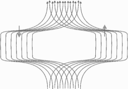
Figure 4: Possible configurations of converging and diverging poloidal magnetic field in the disk and the TL. The left configuration corresponds to the case in which the magnetic pressure at the interface between the disk and the TL increases vertically, and therefore enhances the collapse of the TL. The right case corresponds to magnetic pressure that opposes collapse.

2.4 The profiles of the other variables

1. To have stationary solutions, the energy due to the toroidal magnetic field in the TL must be is in equipartition with the rotational energy, i.e., $E^{\mathrm{T}}_{\mathrm{mag}}=E_{\mathrm{rot}}$. This means that:

   $$V^{\mathrm{T}}_{\mathrm{A}}=\frac{B_{\mathrm{T}}}{\sqrt{\rho}}=V_{\mathrm{\varphi}},\Longrightarrow\rho=(\frac{B_{\mathrm{T}}}{V_{\mathrm{\varphi}}})^{2}=const.\doteq\rho^{0}_{\mathrm{W}}.$$

   Thus the disk must supply the plasma in the TL with the optimal material flux across the interface, so to maintain the density constant.
   When r-integrating the equation of mass conservation, Eq. 7, we obtain:

   $${\,\dot{\cal M}}^{\mathrm{d}}_{\mathrm{r}}={\,\dot{\cal M}}^{\mathrm{d}}_{\mathrm{r=r_{\mathrm{tr}}}}+2\,({\,\dot{\cal M}}^{\mathrm{W}}_{\mathrm{r}}-{\,\dot{\cal M}}^{\mathrm{W}}_{\mathrm{r=r_{\mathrm{tr}}}})={\,\dot{\cal M}}^{\mathrm{d}}_{\mathrm{r=r_{\mathrm{tr}}}}+2\Delta{\,\dot{\cal M}}^{\mathrm{W}}.$$ (17)

   This gives the density profile along the equator:

   $$\rho_{\mathrm{d}}=\frac{{\,\dot{\cal M}}^{\mathrm{d}}_{\mathrm{r}}}{rH_{\mathrm{d}}U_{\mathrm{d}}}=\frac{{\,\dot{\cal M}}^{\mathrm{d}}_{\mathrm{r}}}{\epsilon r^{2}U_{\mathrm{d}}},$$ (18)

   which is a function of radius and of $\rho^{0}_{\mathrm{W}}$.
   The density in the TL then reads:

   $$\rho_{\mathrm{W,0}}=({\,\dot{\cal M}}^{\mathrm{d}}_{\mathrm{r_{\mathrm{tr}}}}-{\,\dot{\cal M}}^{\mathrm{d}}_{\mathrm{r=rin}})r^{-7/4}{\cal F}^{-1}/2,,\,\,{\rm where}\,\,{\cal F}=[\sqrt{r}-1]^{1/2}$$ (19)

   Although $\rho_{\mathrm{W,0}}$ can be treated as an input parameter, we provide here its value relative to the central density at the equator. Taking into account that $U_{\mathrm{W}}$ vanishes at $r_{\mathrm{BL}}$ and applying mass conservation to an adjusting volume cell in the TL, we obtain the rough estimate:

   $$\rho_{\mathrm{W,0}}=[\rho_{\mathrm{\theta_{d}}}][(\frac{V_{\mathrm{\theta_{d}}}}{U^{\mathrm{W}}})][(\frac{r}{H_{\mathrm{W}}}]=[\epsilon\rho_{\mathrm{c}}][\epsilon^{2}][1/\epsilon]=\epsilon^{2}\rho_{\mathrm{d}}(r=r_{\mathrm{BL}}).$$ (20)

   In deriving this result, we have used $V_{\theta_{d}}=\epsilon^{2}U_{\mathrm{d}}$, which relies on asymptotic expansion of the variables $q=q_{0}+\epsilon q_{1}+\epsilon^{2}q_{2}+...$, where $q_{0}$ is the value corresponding to an equilibrium state, i.e., hydrostatic equilibrium in the vertical direction (Regev & Hujeirat, 1988, see the references therein). Thus, replacing ${\partial{\,\dot{\cal M}}^{\mathrm{W}}_{\mathrm{r}}}/{\partial r}$ by ${{\,\dot{\cal M}}^{\mathrm{W}}_{\mathrm{r}}}/{r}$ in Eq. 7, we may obtain a more accurate value for the vertical velocity across the interface at $\theta_{\mathrm{d}}$:

   $$V(r,\theta_{\mathrm{d}})=\frac{\rho^{\mathrm{W}}_{0}r^{5/4}{\cal F}}{[{\,\dot{\cal M}}^{\mathrm{d}}_{\mathrm{0}}-2\rho^{\mathrm{W}}_{0}({\,\dot{\cal M}}^{\mathrm{W}}_{\mathrm{0}}+r^{7/4}{\cal F})]}.$$ (21)

   The outward-oriented material flux compared to the accretion rate is displayed in Fig.7. The corresponding 2D profiles of the poloidal and toroidal components of the velocity field are shown in Fig. 8.

   

   

   

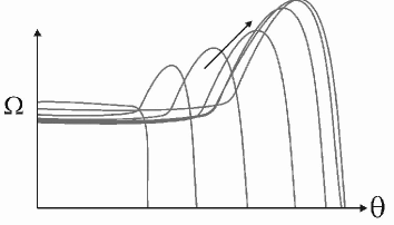
   Figure 5: A schematic description for a time-sequence of the angular velocity profile in the vertical direction. TAWs transport angular momentum vertically, enforcing the matter in the disk to rotate sub-Keplerian, and super-Keplerian in the TL (top). The resulting $\Omega-$profiles acquire negative and positive spatial derivatives (middle), which in the presence of a large scale PMF, generate toroidal flux tubes of opposite signs (bottom) that subsequently reconnect and annihilate.

2. The profile of the magnetic diffusivity in the TL reads: $\nu_{\mathrm{mag}}=H_{\mathrm{W}}V^{\mathrm{T}}_{\mathrm{A}}=\epsilon rB_{\mathrm{T}}/\sqrt{\rho}\sim r^{3/4}.$

3. The ion temperature is obtained by requiring that the advection and heating time scales to be equal, i.e., $\tau_{\mathrm{adv}}=\tau_{\mathrm{heat}}$, where $\tau_{\mathrm{heat}}=C_{\mathrm{V}}\rho T_{\mathrm{i}}/\Phi$. $\Phi$ is the dissipation function: $\nu_{\mathrm{mag}}|\nabla\times B|^{2}\approx\nu_{\mathrm{mag}}B_{\mathrm{T}}^{2}/H^{2}_{\mathrm{W}}$. This gives $T_{\mathrm{i}}\sim r^{-1/2}$, or more accurately,

   $$T_{\mathrm{i}}=T^{0}_{\mathrm{i}}Y^{-1/2}$, where $T^{0}_{\mathrm{i}}=1/\epsilon^{2}.$$ (22)

4. The electron temperature is extremely sensitive to the strength of the magnetic field. Since the heat liberated through magnetic reconnection can heat both the electrons and protons equally, the temperature of the electrons can be found by equalizing the Synchrotron cooling rate to the heating rate. In order to calculate the Synchrotron cooling, we must first find the critical frequency, below which the media becomes optically thick to Synchrotron radiation, i.e, $\nu_{\mathrm{c}}$, below which the emission follow the Raleigh-Jeans blackbody emissivity profile. This requires solving the equation:

   $$\int{\varepsilon^{\nu}}\,dVol=\int{B_{\nu}}d\,S,$$ (23)

   where $\varepsilon^{\nu}$ and $B_{\nu}$ are the Synchrotron and Raleigh-Jeans blackbody emissivities, respectively. Having calculated $\nu_{\mathrm{c}}$, the Synchrotron cooling $\Lambda_{\mathrm{syn}}$ is then calculated by dividing the total luminosity from the surface of the TL divided by its corresponding volume-integrated frequency from $\nu=0$ up to $\nu_{\mathrm{c}}$, where the medium is assumed to be self-absorbed for $\nu\leq\nu_{\mathrm{c}}$. This gives Esin et al. (1996):

   $$\Lambda_{\mathrm{syn}}\approx\frac{2\pi kT_{e}\nu^{3}_{\mathrm{c}}}{3H_{\mathrm{W}}c^{2}}.$$ (24)

   Synchrotron emission at higher frequencies is assumed to be negligibly small. In terms of the density and magnetic fields, the following approximation due to can be used Shapiro & Teukolsky (1983):
   $\Lambda_{\mathrm{syn}}=2.16\times 10^{4}B^{2}_{3}T^{2}_{9}\rho_{10},$ where $B_{3}=B/10^{3}G$, $T_{9}=T/10^{9}K$ and $\rho_{10}=\rho/10^{-10}gr.$
   Therefore, from the equalizing the heating to cooling rate, we obtain the following profile for the electron temperature: $T_{\mathrm{e}}=T^{0}_{\mathrm{e}}\,Y^{-5/8},$ and $T^{0}_{\mathrm{e}}=1/\epsilon.$

5. It should be stressed here that only a small fraction of the total generated TMF is allowed to undergo magnetic reconnection in the TL. This is an essential requirement for not obtaining radio luminosity that dominate the total power emerging from jet-bases, and to assure that the outflow is associated with TMF-energy sufficient enough for collimating the outflows into jets. Thus, comparing the rate of heating via magnetic reconnection with the generation rate of the TMF, we obtain:

   $$\frac{(1/\tau_{\mathrm{Diss}})}{(1/\tau_{\mathrm{gen}})}=\frac{\tau_{\mathrm{gen}}}{\tau_{\mathrm{Diss}}}=\epsilon(\frac{B_{\mathrm{T}}}{B_{\mathrm{p}}})(\frac{\nu_{\mathrm{mag}}}{H_{\mathrm{W}}V_{\mathrm{\varphi}}})=\frac{\sqrt{2}\alpha_{\mathrm{mag}}}{\log(Re)}\approx\epsilon,$$ (25)

   where we have used $\nu_{\mathrm{mag}}=H_{\mathrm{W}}V^{T}_{\mathrm{A}}$ and $B_{\mathrm{p}}/B_{\mathrm{T}}=H_{\mathrm{W}}/r=\epsilon$. Consequently, an $\epsilon-$fraction of the total generated toroidal magnetic energy undergoes magnetic reconnection, while the rest is advected with the relativistic outflow.

We now turn to find out the appropriate profiles of the electron- and proton-temperatures in the disk region.

Figure 6: The profiles of $\bar{\alpha}Re$ and $\log{Re}$ versus the magnetic Reynolds number $Re$, where $\bar{\alpha}=\alpha_{\mathrm{mag}}(\frac{B_{\mathrm{T}}}{B_{\mathrm{p}}})$. The intersection point $Re^{\mathrm{c}}$ corresponds to the solution of Equation 14.

The electrons in the disk region are heated mainly by adiabatic compression, conduction and by other non-local energy sources. However, they may suffer of an extensive cooling due Synchrotron emission. We assume that at the interface between the disk and the TL, there is a conductive flux that is sufficiently large so to compensate the cooling of the disk-electrons through Synchrotron emission. In other wards, we require that $\tau_{\mathrm{Syn}}=\tau_{\mathrm{heat}}$. In this case the electron temperature adopts the adiabatic profile; $T_{\mathrm{e}}\sim r^{-1}.$

How does the ion-temperature correlate with that of the electrons in the disk region?
Assume that the electrons and the protons to have Maxwell velocity distributions. The time scale required to establish an equilibrium Spitzer (1956) is:

$$\tau_{\mathrm{therm}}=4.11(T_{9}^{3/2}/n_{14})(20/ln{\Lambda})\,s,$$ (26)

where $T_{9}=T/10^{9}\,K$, and the proton number density is given as $n_{14}=n/10^{14}$. Therefore, in the disk region $\tau_{\mathrm{therm}}$ is of the same order as or greater than the hydrodynamical time scale if $n\geq 10^{10}$, which implies that $T_{\mathrm{e}}\approx T_{p}$ for reasonable accretion rates. In the transition layer, however, $n(TL)\sim\epsilon^{2}n(disk)$. Therefore $T_{\mathrm{e}}$ and $T_{p}$ can be significantly different.

Figure 7: The radial profiles of the accretion rate in the disk region, and the outwards-oriented material flux in the launching layer, $F_{\mathrm{outflow}},$ which applies for $r\leq r_{\mathrm{tr}}$. Note that $F_{\mathrm{outflow}}$ vanishes at the inner boundary $r_{\mathrm{BL}}$, where the effective gravity is set to vanish. Assuming $\epsilon=0.1=H_{\mathrm{d}}/r$, the maximum material flux associated with the outflow is approximately 5% of the total accretion rate through the outer boundary. Thus, $F_{\mathrm{outflow}}$ depends on the disk temperature; colder disks yield lower $F_{\mathrm{outflow}}$ and vice versa.

3 Electron-positron versus electron-proton jets

Since the flow in the TL is heated through magnetic reconnection, it is naturally to ask whether it is $e^{-}/e^{+}-$ or $e^{-}/p-$dominated plasma.
In view of the solar flares, we may expect the plasma in the TL to accommodate different plasma-populations such as electron-positron, electron-proton in a see of high $\gamma-$rays. The relativistic acceleration that particles experience during reconnection events in the vicinity of the BH give rise to different types of pair creation, in particular $\gamma-\gamma$, $\gamma-e^{\mp}$, $e^{\mp}-e^{\mp}$, $\gamma-p$, $e^{\mp}-p$ Svensson (1982); Björnsson & Svensson (1991); White & Lightman (1989). Among other effects, pair fraction depends crucially on two important parameters: the optical depth to scattering and on the so called compactness parameter. The latter parameter is a fundamental scaling quantity for relativistic plasmas having $\vartheta=kT_{\mathrm{e}}/m_{\mathrm{e}}c^{2}$ is of order unity.
Taking into account that the plasma in the innermost region of the disk is freely falling, and that ${\,\dot{\cal M}}_{\mathrm{d}}=2H_{\mathrm{d}}r<\rho_{\mathrm{d}}>U$, we obtain that the optical depth to scattering in the innermost part of disk is:

$$\tau^{\mathrm{d}}_{\mathrm{s}}=\frac{\kappa_{s}{\,\dot{\cal M}}_{\mathrm{d}}}{2rU}=18.86(\frac{r}{r_{\mathrm{LSO}}})^{-1/2}(\frac{{\,\dot{\cal M}}}{{\,\dot{\cal M}}_{\mathrm{Edd}}}),$$ (27)

where $r_{\mathrm{LSO}}$ is the last stable radius. Noting that $\rho_{\mathrm{W}}=\epsilon^{2}\rho_{\mathrm{d}}$, and that the optical depth obeys a similar relation, i.e., $\tau^{\mathrm{W}}_{\mathrm{s}}=\epsilon^{2}\tau^{\mathrm{d}}_{\mathrm{s}}$, we may conclude that the TL is optically thin to scattering for most accretion rate typical for AGNs. Further, since the flow in the TL is steady and two-temperature, our models fall in the left-down corner of the $\tau_{\mathrm{s}}-{\,\dot{\cal M}}$ diagram of in Fig. 10 of Esin (1999), from which we conclude that jets are formed in ion/proton-dominated plasma.

4 Extraction of rotational energies from the BH and from the disk

A spinning black hole is surrounded by the so called ergosphere, inside which no static observer is possible; any frame of reference must be dragged by the spin of the black hole. If the plasma in the ergosphere is threaded by an external and ordered magnetic field, then the MF-lines must be dragged as well, thereby generating an electric field $\@vec{E}=\@vec{V}\times\@vec{B}$. In the ergosphere, however, negative energy orbits are possible (i.e., the total energy including the rest mass of the particle is negative). If a PMF threads the event horizon, it can put particles on negative energy orbits. These particles will be swallowed by the BH, while other particles with positive energy will emerge that carry electromagnetic energy flux from the hole. These extracted energies from the hole is used then to accelerate the plasma-particles relativistically, possibly forming $e^{-}/e^{+}-$dominated jets (see Blandford & Znajek, 1977; Rees et al., 1982; Begelman et al., 1984). The direction and magnitude of the electromagnetic flux are described by the Poynting vector:

$$\@vec{P}=-\frac{1}{4\pi}E\times B=-\frac{1}{4\pi}V\times B\times B.$$ (28)

Using spherical geometry, the components of the Poynting flux read:

$$\begin{array}[]{ll}\@vec{P}=-\frac{1}{4\pi}\{&(V_{\mathrm{\varphi}}B_{\mathrm{r}}B_{\mathrm{T}}-V_{\mathrm{r}}B_{\mathrm{T}}^{2}-V_{\mathrm{r}}B_{\mathrm{\theta}}^{2}+V_{\mathrm{\theta}}B_{\mathrm{r}}B_{\mathrm{\theta}}),\\ &(V_{\mathrm{r}}B_{\mathrm{r}}B_{\mathrm{\theta}}-V_{\mathrm{\theta}}B_{\mathrm{r}}^{2}-V_{\mathrm{\theta}}B_{\mathrm{T}}^{2}-V_{\mathrm{\varphi}}B_{\mathrm{T}}^{2}),\\ &(V_{\mathrm{\theta}}B_{\mathrm{\theta}}B_{\mathrm{T}}-V_{\mathrm{\varphi}}B_{\mathrm{\theta}}B_{\mathrm{T}}-V_{\mathrm{\varphi}}B_{\mathrm{r}}^{2}+V_{\mathrm{r}}B_{\mathrm{r}}B_{\mathrm{T}})\}.\end{array}$$ (29)

In the case of a spinning BH surrounded by a plasma with zero poloidal motion, i.e., $V=V_{\mathrm{r}}=V_{\mathrm{\theta}}=0$, a PMF of external origin in the vicinity of the event horizon is predominantly radial, or equivalently, it has a monopole-like topology. In this case the Poynting flux reads:

$$\@vec{P}^{\mathrm{BH}}\approx-\frac{1}{4\pi}(V_{\mathrm{\varphi}}B_{\mathrm{r}}B_{\mathrm{T}},0,0)$$ (30)

The corresponding electromagnetic luminosity carried out off the black hole reads:

$$L^{\mathrm{BH}}=\int{\@vec{P}^{\mathrm{BH}}_{\mathrm{r}}\cdot dS}=\frac{1}{4}r_{\mathrm{H}}^{2}V_{\mathrm{\varphi}}B_{\mathrm{r}}B_{\mathrm{T}},$$ (31)

where $r_{\mathrm{H}}$ is the event horizon.

Similarly, applying the same procedure to the plasma in the TL, neglecting the effects of vertical advection, and noting that $B_{\mathrm{p}}=\epsilon B_{\mathrm{T}}$, then the Poynting flux is predominantly radial:

$$\@vec{P}^{\mathrm{TL}}\approx\@vec{P}^{\mathrm{TL}}_{\mathrm{r}}=-\frac{1}{4\pi}(V_{\mathrm{r}}B_{\mathrm{T}}^{2},0,0).$$ (32)

The corresponding luminosity is obtained then by integrating the flux over the radial surface of the TL at $r=r_{\mathrm{tr}}$:

$$L^{\mathrm{TL}}=\int{\@vec{P}^{\mathrm{TL}}_{\mathrm{r}}\cdot dS}=r_{\mathrm{tr}}H_{\mathrm{W}}V_{\mathrm{r}}B_{\mathrm{T}}^{2}.$$ (33)

Thus, the ratio of the above two luminosities yields:

$$\frac{L^{\mathrm{BZ}}}{L^{\mathrm{TL}}}=\frac{1}{4\epsilon}(\frac{V_{\mathrm{\varphi}}^{\mathrm{BH}}}{V_{\mathrm{r}}^{\mathrm{tr}}})(\frac{B_{\mathrm{r}}^{\mathrm{BH}}}{B_{\mathrm{T}}^{\mathrm{tr}}})(\frac{B_{\mathrm{T}}^{\mathrm{BH}}}{B_{\mathrm{T}}^{\mathrm{tr}}})(\frac{r_{\mathrm{H}}}{r_{\mathrm{tr}}})^{2}.$$ (34)

How large this ratio is, depends strongly on the location of the transition radius $r_{\mathrm{tr}}$. We now turn to estimate the transition radius $r_{\mathrm{tr}}$.
Noting that at $r_{\mathrm{tr}}$ the magnetic energy is in equipartition with the thermal energy of the disk-plasma which, in terms of Eq. A.2, means that:

$$\frac{1}{r_{\mathrm{tr}}^{2}}=\frac{1}{\rho}\frac{\partial}{\partial r}B_{\mathrm{\theta}}^{2}.$$ (35)

Furthermore, noting that $r_{\mathrm{BL}}$ is the critical radius where $B_{\mathrm{p}}$ change topology, and where the corresponding magnetic energy is roughly in equipartition with rotational energy, we obtain from Eq. A.2:

$$\frac{1}{\epsilon^{2}}\frac{1}{r_{\mathrm{BL}}^{2}}=\frac{1}{\rho}\frac{\partial}{\partial r}B_{\mathrm{\theta}}^{2}.$$ (36)

Taking into account the spatial variations of $B_{\mathrm{p}}$ and $\rho$ as described in Equations 47 and 50, and solving for X at $r_{\mathrm{BL}}$, we find that:

$$X(r=r_{\mathrm{BL}})=\epsilon^{4/3}\approx\left\{\begin{array}[]{lll}0.046&\leavevmode\nobreak\ \leavevmode\nobreak\ \leavevmode\nobreak\ \leavevmode\nobreak\ \leavevmode\nobreak\ \leavevmode\nobreak\ {\rm if}\leavevmode\nobreak\ \epsilon=10^{-1}&(\longrightarrow r_{\mathrm{tr}}\approx 20)\\ 0.018&\leavevmode\nobreak\ \leavevmode\nobreak\ \leavevmode\nobreak\ \leavevmode\nobreak\ \leavevmode\nobreak\ \leavevmode\nobreak\ {\rm if}\leavevmode\nobreak\ \epsilon=5\times 10^{-2}&(\longrightarrow r_{\mathrm{tr}}\approx 50)\\ 0.002&\leavevmode\nobreak\ \leavevmode\nobreak\ \leavevmode\nobreak\ \leavevmode\nobreak\ \leavevmode\nobreak\ \leavevmode\nobreak\ {\rm if}\leavevmode\nobreak\ \epsilon=10^{-2}&(\longrightarrow r_{\mathrm{tr}}\approx 500),\end{array}\right.$$ (37)

where $r_{\mathrm{tr}}$ is given in $r_{\mathrm{BL}}-$units. Using Eq. 34, and taking into account the spatial variations of $U_{\mathrm{W}}$ and $B_{\mathrm{T}}$ in the TL, and assuming that the central BH is rotating at maximum rate, we may obtain the following inequality inequality:

$$\frac{L^{\mathrm{BZ}}}{L^{\mathrm{TL}}}\leq\frac{1}{4\epsilon}{Y^{3/4}}(\frac{r_{\mathrm{H}}}{r_{\mathrm{tr}}})^{2}=\frac{1}{4\epsilon}(\frac{r_{\mathrm{H}}}{r_{\mathrm{tr}}})^{5/4},$$ (38)

which is larger than $5\%$ for most reasonable values of $\epsilon(>10^{-3})$.
Consequently, the TL appears to provide the bulk of the electromagnetic energy associated with jets, even when the central BH is maximally rotating. The contribution of the BHs to the total electromagnetic energy flux is significant, but it is unlikely to be dominant.
Thus, the total power available from the launching layer and from the spinning BH is:

$$L_{\mathrm{tot}}=L_{\mathrm{TL}}+L_{\mathrm{BZ}}=L_{\mathrm{TL}}(1+\frac{1}{4\epsilon}(r_{\mathrm{H}}/r_{\mathrm{tr}})^{5/4}).$$ (39)

If the accretion rate is relatively large and the BH rotates at maximum rate, $\tau_{\mathrm{TAW}}$, becomes longer than $\tau_{\mathrm{dyn}}$, and therefore $r_{\mathrm{tr}}$ must move toward smaller radii. Consequently, the ratio ${L^{\mathrm{BZ}}}/{L^{\mathrm{TL}}}$ increases, but remains below 25% of the total available luminosity from the TL for most reasonable values of accretion rates.

We note that $r_{\mathrm{tr}}$ in our present consideration serves as a lower limit. The reason is that the rate of turbulence generation is likely to starts decreasing when the ratio of the magnetic to internal energies exceeds the saturation value that has been revealed by MHD calculations Hawley et al. (1996), and is likely to suffer of a complete suppression at $r_{\mathrm{tr}}$, where $\beta$ starts to exceed unity.

Figure 8: The distribution of the velocity field in the transition region superposed on equally-spaced isolines of the angular velocity $\Omega$. The strong-decrease of $\Omega$ with radius in the equatorial region relative to its slow-decrease in the TL is obvious. The overlying dynamically unstable corona is rotation-free. The orange colour corresponds to large material densities, violet to intermediate and blue correspond to extremely tenuous coronal plasma. The 2D distributions of the variable have been obtained using a vertical interpolation procedure.

Figure 9: 20 equally-spaced isolines of the poloidal-component $\rm B_{\mathrm{P}}$ (white contours), superposed on the coloured-distribution of the toroidal magnetic field. Blue, green and red colours correspond to low, intermediate and to high TMF-values, respectively.

5 Luminosity of truncated disks

The primary source of heating in standard disks is due to dissipation of turbulence. The corresponding heating function reads: Frank et al. (1992):

$$D(r)=\frac{1}{2}\eta_{\mathrm{tur}}(r\frac{\partial\Omega}{\partial r})^{2},$$ (40)

where $\eta_{\mathrm{tur}}=\Sigma\nu_{\mathrm{tur}}$, $\Sigma$ is surface density, and $\nu_{\mathrm{tur}}$ is the standard turbulent viscosity.
Following the analysis of Frank et al. (1992), the r-integrated time-independent equation of angular momentum in one-dimension reads:

$$\Sigma U\Omega=\eta_{\mathrm{tur}}\frac{\partial\Omega}{\partial r}+C/2\pi r^{3},$$ (41)

where C is an integration constant. The classical assumption was that $\partial\Omega/\partial r$ must vanishes at some radius close to the central object, and so imposing a physical constrain on C. The idea here was motivated by the two observationally supported assumptions: 1) Almost all astrophysical objects, that so far have been observed, are found to rotate at sub-Keplerian rates, and 2) $\nu_{\mathrm{tur}}$ is a non-vanishing function/process.
In the recent years, however, two possibilities have emerged: 1) several accretion disk in AGNs appear to truncate at radii much larger than their gravitational radii, 2) magnetic fields in accretion disks can be amplified by the Balbus-Hawley instability, and potentially they may reach thermal equipartition, beyond which local random motions, turbulence-generation as well as turbulence dissipation are suppressed.
Therefore, we may think of C as some sort of a magnetic effect that come into play whenever the accretion flow approaches a certain radius $r_{\mathrm{tr}}$ from outside, at which turbulence generation is diminished. In view of Equation 41, we obtain:

$$\eta_{\mathrm{tur}}=\frac{{\,\dot{\cal M}}}{3\pi}[1-(\frac{r_{\mathrm{tr}}}{r})^{1/2}]\Longrightarrow D(r)=\frac{3GM{\,\dot{\cal M}}}{8\pi r^{3}}[1-(\frac{r_{\mathrm{tr}}}{r})^{1/2}],$$ (42)

which applies for $r\geq r_{\mathrm{tr}}$ only. The corresponding luminosity reads:

$$L=2\int^{\mathrm{r_{\mathrm{tr}}}}_{\infty}D(r)2\pi rdr=\frac{1}{2}\frac{GM{\,\dot{\cal M}}}{r_{\mathrm{tr}}}.$$ (43)

In the case of the nucleus in M87, if the disk surrounding the BH truncates at 100 gravitational radii, then the corresponding accretion luminosity is:

$$L\approx\frac{GM{\,\dot{\cal M}}}{2R_{tr}}=\frac{GM{\,\dot{\cal M}}}{200\,R_{g}}=2.5\times 10^{-3}c^{2}{\,\dot{\cal M}}=2.5\times 10^{-6}c^{2}{\,\dot{\cal M}}_{\mathrm{Edd}}\approx 10^{42}erg\,s^{-1},$$ (44)

where ${\,\dot{\cal M}}=1.6\times 10^{-3}{\,\dot{\cal M}}_{\mathrm{Edd}}$ has been used Di Matteo et a. (2003).
Thus, the jet power should of the order of:

$$L_{\mathrm{J}}=\frac{GM{\,\dot{\cal M}}}{2r_{BL}}-\frac{GM{\,\dot{\cal M}}}{2r_{BL}}\approx\frac{GM{\,\dot{\cal M}}}{2R_{BL}}\approx 10^{44}erg\,s^{-1},$$ (45)

which agrees with the observations (see Bicknill & Begelman, 1999). In writing Eq. 45, we have assumed that $r_{\mathrm{BL}}$ is located very close to the last stable orbit.
Consequently, interior to $r_{\mathrm{tr}}$ the energy goes primarily into powering the jet with magnetic and rotational energies. This power dominate the luminosity of the truncated disk, making it difficult to observe the disk directly.

6 Discussion

In this paper we have presented a theoretical model for accretion-powered jets in AGNs and microquasars. The model relies primarily on electromagnetic extraction of rotational energy from the disk-plasma and the formation of a geometrically thin launching layer between the disk and the overlying corona.
The model is based on self-similar solution for the 3D axi-symmetric radiative two-temperature MHD equations. The very basic assumption underlying this model is that standard disks should truncate energetically at a certain radius $r_{\mathrm{tr}}$, below which $B_{\mathrm{p}}$ start to increase inwards as $r^{-2}$, and eventually becomes in excess of thermal equipartition. Thus, the matter and the frozen-in PMF can be accreted by the BH as far as TAWs are able to efficiently extract rotational energy normal to the disk. Such a flow-configuration can be maintained if the PMF change topology at $r_{\mathrm{BL}}$, which must be associated with loss of magnetic flux, so to avoid complete termination of accretion. Moreover, unlike standard disks in which the accretion energy is liberated away, or advected inwards as entropy (ADAF solutions), the accretion energy here is converted mainly into magnetic energy that power the jet. In this case, the plasma in the innermost part of the disk becomes: 1) turbulent-free, 2) rotates sub-Keplerian, and 3) remains relatively cold and confined to a geometrically thin disk. On the other hand, the plasma in the TL rotates super-Keplerian, dissipative, two-temperature, virial-hot and ion-dominated.
To first order in $\epsilon$, the profiles of the main variables in the disk are:

$$U_{\mathrm{d}}(r)=[U^{2}_{\mathrm{0,d}}+\frac{2}{\epsilon^{2}}(\frac{1}{X}-1)]^{1/2},$$ (46)

$$\rho_{\mathrm{d}}(r)=\rho^{0}_{\mathrm{d}}{\cal F}_{\rho}X^{-3/2},$$ (47)

$$\Omega_{\mathrm{d}}(r)=\Omega^{0}_{\mathrm{d}}X^{-5/4},$$ (48)

$$T_{\mathrm{d}}(r)=T^{0}_{\mathrm{d}}X^{-5/8},$$ (49)

$$B_{\mathrm{p,d}}(r)\approx B_{\mathrm{\theta,d}}(r)=B^{0}_{\mathrm{d}}X^{-2},$$ (50)

where $X=r/r_{\mathrm{tr}}$, ${\cal F}_{\rho}=[({\,\dot{\cal M}}^{0}_{\mathrm{d}}+2\Delta{\,\dot{\cal M}}_{\mathrm{W}})/\epsilon U_{\mathrm{d}}]r_{\mathrm{tr}}^{-3/2}r^{-1/2}$ (see Eq. 17), $\rho^{0}_{\mathrm{d}}=\alpha^{-7/10}_{\mathrm{tur}}{\,\dot{\cal M}}^{11/20}r^{-15/8}f^{11/5}$, $\Omega^{0}_{\mathrm{d}}=r_{\mathrm{tr}}^{-3/2}$ and $B^{0}_{\mathrm{d}}=\sqrt{\rho^{0}_{\mathrm{d}}T^{0}_{\mathrm{d}}}$. Note that the superscript ‘0’ and the subscript ‘d’ denote the values at the equator and at $r_{\mathrm{tr}}$, and which be found using standard accretion disk theory.

In the launching region the variables have the following profiles:

$$U^{\mathrm{W}}(r)=\frac{\sqrt{2}}{\epsilon}(1-\frac{1}{\sqrt{Y}})^{1/2}r_{\mathrm{tr}}^{-1/4},$$ (51)

$$\rho^{\mathrm{W}}(r)=const.=\frac{\epsilon{\,\dot{\cal M}}^{0}_{\mathrm{d}}}{r^{2}U_{\mathrm{d}}-2\sqrt{2}\epsilon\Delta_{0}}|_{r=r_{\mathrm{BL}}},$$ (52)

$$\Omega^{\mathrm{W}}(r)=\Omega^{0}_{\mathrm{W}}Y^{-5/4},$$ (53)

$$T^{\mathrm{i}}_{\mathrm{W}}(r)=T^{\mathrm{i}}_{\mathrm{W,0}}Y^{-1/2},\,\,\,T^{\mathrm{e}}_{\mathrm{W}}(r)=T^{\mathrm{e}}_{\mathrm{W,0}}Y^{-5/8}$$ (54)

$$B_{\mathrm{p,W}}(r)=B^{0}_{\mathrm{p,W}}Y^{-2},$$ (55)

$$B_{\mathrm{T,W}}(r)=B^{0}_{\mathrm{T,W}}Y^{-1/4},$$ (56)

where $Y=r/r_{\mathrm{BL}}$, $\Delta_{0}=[(r^{7/4}{\cal F})-(r^{7/4}{\cal F})_{r=r_{\mathrm{tr}}}]$, $\Omega^{0}_{\mathrm{W}}=r_{\mathrm{BL}}^{-3/2}$, $T^{\mathrm{i}}_{\mathrm{W,0}}=1/\epsilon^{2}$, $T^{\mathrm{e}}_{\mathrm{W,0}}=1/\epsilon$, $B^{0}_{\mathrm{p,W}}=1/\epsilon^{2}$ and $B^{0}_{\mathrm{T,W}}=1/\epsilon^{2}$. The variables here are given in the units listed in Table A.1 (see Appendix).

Furthermore, we would like to point out that:

1. Magnetic reconnection in combination with Joule heating is an essential ingredient for our model to work. The magnetic diffusivity adopted here, $\nu_{\mathrm{mag}}=H_{\mathrm{W}}V^{\mathrm{T}}_{\mathrm{A}}$, is proportional to $V^{\mathrm{T}}_{\mathrm{A}}$, and therefore it vanishes at turning points where $B_{\mathrm{T}}$ changes its sign. This prescription does not smooth the $B_{\mathrm{T}}-$gradients on the account of Joule-heating the plasma, but it strengthen the $B_{\mathrm{T}}-$gradients even more, thereby enhancing the rate of $B_{\mathrm{T}}-$reconnection. The underlying idea here is not to smooth the $B_{\mathrm{p}}-$gradients, but to terminate the propagation of the TAWs to higher latitudes, trapping therefore the angular momentum in the TL. In general, a normal magnetic diffusivity cannot hinder the propagation of TAWs into the corona.

2. If the axi-symmetric assumption is relaxed, there might be still ways to transport angular momentum from the disk into the corona without forming a dissipative TL. Such ways can be explored using a full 3D implicit radiative MHD solver, taking into account Bremsstrahlung and Synchrotron coolings, heat conduction, and able to deal with highly stretched mesh distributions. Such solvers are not available to date, and therefore beyond the scope of the present paper. On the other hand, since the region of interest is located in the vicinity of an axi-symmetric black hole, the axi-symmetric assumption might be a valid description for the flow in the TL and in the disk. Furthermore, in the absence of heating from below, coronae around black holes have been found to be dynamically unstable to heat conduction Hujeirat et al. (2002). In order to hold a BH-corona against dynamical collapse, the MFs threading the corona must be sufficiently strong. These, in turn, force the gyrating electrons to cool rapidly through emitting Synchrotron radiation. In the absence of efficient heating mechanisms for the plasma in the corona, this cooling may even runaway.
   Consequently, coronae around BHs most likely will diminish, and the robust way to form jets would be through the formation of a TL, which might be a natural consequence of accretion flows onto BHs.

3. We note that if the innermost part of the disk is threaded by an $r^{-2}-$PMF, then $\Omega\sim r^{-5/4}$ is likely to be the optimal profile for the angular velocity. Specifically,

   1. $\Omega\sim r^{-5/4}$ satisfies Eq. 25, so that $\alpha_{\mathrm{mag}}$, and hence ${\,\dot{\cal M}}$ can be fine-tuned so to produce the radio luminosity and jet-power that agrees with observations.

   2. Multi-dimensional radiative MHD calculations have shown that $r^{-5/4}$ is the appropriate profile for the angular velocity in the TL Hujeirat et al. (2003).

   3. Conservation of angular momentum implies that the flow in the disk must be advective-dominated to be able to supply the plasma in the TL with angular momentum, so to maintain the $r^{-5/4}-$profile.

   4. The Keplerian profile $\Omega=cr^{-3/2}$, with c=1 yields slow accretion. In this case, the cooling time scales will be faster than the hydrodynamical time scale. Thus, the disk cools and the matter settles into a standard disk. However, such a disk is unlikely to be stable if the PMFs is in super-equipartition with the thermal energy.
      If $c<1$, then $r_{\mathrm{tr}}$ must move to much larger radii, and as $B_{\mathrm{p}}$ increases inwards as $r^{-2}$, accretion may terminate by the magnetic pressure.

   5. Adopting the profile $\Omega\sim r^{-1}$ does not fulfil Eq. 25, which requires that the bulk of the generated TMF-energy must be advected with the outflow. Moreover, this profile yields unacceptably large and radius-independent toroidal magnetic field in the transition layer, and so overestimating the radio luminosity.

4. The transition radius $r_{\mathrm{tr}}$, which is treated as input parameter, depends strongly on the accretion rate. If the outer disk fails to supply its innermost part with a constant accretion rate, then the flow may become time-dependent. In this case, the emerging plasmas does not show up as continuous jet, but rather in a blob-like configuration. A high ${\,\dot{\cal M}}$ gives rise to $\tau_{\mathrm{TAW}}>\tau_{\mathrm{hd}}$ so that $r_{\mathrm{tr}}$ must move towards smaller radii. In this case, the total rotational power extracted from the innermost part of the disk via TAWs becomes smaller, giving rise thereby to a less energetic and weakly collimated jets. On the other hand, a low ${\,\dot{\cal M}}$ would allow $r_{\mathrm{tr}}$ to move outwards, the total surface from which angular momentum is extracted is larger, and the resulting jets are more energetic, have larger magnetic and rotational energies and therefore are more collimated.

5. We have shown that the BZ-process modifies the total power of the jet. However, we have verified also that the extraction of rotational energy from the innermost part of the disk continue to dominate the total power available from the disk-BH system.

Finally, in a future work, we intend to implement our model to study the jet-disk connection in the microquasar GRS 1915-105 in the radio galaxy M87.

Appendix A

Scaling variables
Mass:	$\tilde{\cal M}=3\times 10^{8}M_{\odot}$
Accretion rate:	$\tilde{{\,\dot{\cal M}}}=10^{-3}{\,\dot{\cal M}}_{Edd}$
Distance:	$\tilde{R}=R_{\mathrm{in}}=3R_{\mathrm{S}},$ where $R_{\mathrm{S}}=2G\tilde{\cal M}/c^{2}$
Temperature:	$\tilde{\cal T}=5\times 10^{7}K$
Velocities:	$\tilde{V}=\tilde{V_{\mathrm{S}}}=[\gamma{\cal R}_{\mathrm{gas}}\tilde{\cal T}/\mu_{\mathrm{i}}]^{1/2},\,\mu_{\mathrm{i}}=1.23$
Ang. Velocity:	$\tilde{V_{\mathrm{\varphi}}}=\tilde{V_{\mathrm{Kep}}}=(G\tilde{\cal M}/\tilde{R})^{1/2}$, $\Longrightarrow\epsilon=\tilde{V_{\mathrm{S}}}/\tilde{V_{\mathrm{\varphi}}}$
Magnetic Fields:	$\tilde{B}=\tilde{V_{\mathrm{S}}}/\sqrt{4\pi\tilde{\rho}}$
Density:	$\tilde{\rho}=\tilde{{\,\dot{\cal M}}}/(\tilde{H_{\mathrm{d}}}\tilde{R_{\mathrm{out}}}\tilde{V_{\mathrm{S}}})$ $=2.5\times 10^{-12}g\,cm^{-3}$

Table 1: The scaling variables used to reformulate the equations in non-dimensional form.

We use spherical geometry to describe the inflow-outflow configuration around a Schwarzschild black hole. The flow is assumed to be 3D axi-symmetric, and the two-temperature description is used to study the energetics of the ion- and electron-plasmas.
In the following we present the set of equations in non-dimensional form using the scaling variables listed in Table A.1.

1. The continuity equation:

   $$\frac{\partial\rho}{\partial t}+\frac{1}{r^{2}}\frac{\partial}{\partial r}{(r^{2}\rho U)}+\frac{1}{r\cos{\theta}}\frac{\partial}{\partial\theta}{(\cos{\theta}\rho V)}=0$$ (57)

2. The radial momentum equation:

   $$\frac{\partial U}{\partial t}+{U}\frac{\partial U}{\partial r}+\frac{V}{r}\frac{\partial U}{\partial\theta}=\frac{1}{\rho}\frac{\partial P}{\partial r}+\frac{1}{\epsilon^{2}}(r\Omega^{2}-\frac{1}{r^{2}})$$

   $$+\frac{1}{\rho}\frac{B_{\mathrm{\theta}}}{r}\frac{\partial}{\partial\theta}B_{\mathrm{r}}-\frac{1}{\rho}\frac{1}{r}\frac{\partial}{\partial r}(rB_{\mathrm{\theta}}^{2})-\frac{1}{\rho}\frac{1}{r}\frac{\partial}{\partial r}(rB_{\mathrm{T}}^{2})$$ (58)

3. The vertical momentum equation:

   $$\frac{\partial V}{\partial t}+{U}\frac{\partial V}{\partial r}+\frac{V}{r\cos{\theta}}\frac{\partial V}{\partial\theta}=\frac{1}{r\rho}\frac{\partial P}{\partial\theta}-\frac{1}{\epsilon^{2}}\tan{\theta}\frac{V_{\mathrm{\varphi}}^{2}}{r}$$

   $$-\frac{1}{\rho}\frac{B_{\mathrm{r}}}{r}\frac{\partial rB_{\mathrm{\theta}}}{\partial r}-\frac{1}{2r\rho}\frac{\partial}{\partial\theta}(B_{\mathrm{r}}^{2}+B_{\mathrm{T}}^{2})$$ (59)

4. The angular momentum equation:

   $$\frac{\partial\ell}{\partial t}+\frac{1}{r^{2}}\frac{\partial}{\partial r}{(r^{2}\rho U\ell)}+\frac{1}{r\cos{\theta}}\frac{\partial}{\partial\theta}{(\cos{\theta}V\ell)}=B_{\mathrm{\theta}}\frac{\partial B_{\mathrm{T}}}{\partial\theta}+B_{\mathrm{r}}\frac{\partial rB_{\mathrm{\theta}}}{\partial r}$$

   $$+\frac{\cos{\theta}^{2}}{r^{2}}\frac{\partial}{\partial r}({r^{4}\rho\nu_{\mathrm{tur}}\frac{\partial\Omega}{\partial r}})+\frac{1}{\cos{\theta}}\frac{\partial}{\partial\theta}({\cos{\theta}^{3}\rho\nu_{\mathrm{tur}}\frac{\partial\Omega}{\partial\theta}})$$ (60)

5. The internal equation of the ions:

   $$\frac{\partial{\cal E}^{\mathrm{d}}_{\mathrm{i}}}{\partial t}+\frac{1}{r^{2}}\frac{\partial}{\partial r}{(r^{2}\rho U{\cal E}^{\mathrm{d}}_{\mathrm{i}})}+\frac{1}{r\cos{\theta}}\frac{\partial}{\partial\theta}{(\cos{\theta}V{\cal E}^{\mathrm{d}}_{\mathrm{i}})}=-(\gamma-1){\cal E}^{\mathrm{d}}_{\mathrm{i}}\nabla\cdot V$$

   $$+(\gamma-1)\Phi-\Lambda_{\mathrm{i-e}}+\nabla\cdot\kappa^{\mathrm{cond}}_{\mathrm{i}}\nabla T_{\mathrm{i}}$$ (61)

6. The internal equation of the electrons:

   $$\frac{\partial{\cal E}^{\mathrm{d}}_{\mathrm{e}}}{\partial t}+\frac{1}{r^{2}}\frac{\partial}{\partial r}{(r^{2}\rho U{\cal E}^{\mathrm{d}}_{\mathrm{e}})}+\frac{1}{r\cos{\theta}}\frac{\partial}{\partial\theta}{(\cos{\theta}V{\cal E}^{\mathrm{d}}_{\mathrm{e}})}=-(\gamma-1){\cal E}^{\mathrm{d}}_{\mathrm{e}}\nabla\cdot V$$

   $$+(\gamma-1)\Phi+\Lambda_{\mathrm{i-e}}-\Lambda_{\mathrm{\rm B}}-\Lambda_{\mathrm{\rm C}}-\Lambda_{\mathrm{\rm Syn}}+\nabla\cdot\kappa^{\mathrm{cond}}_{\mathrm{e}}\nabla T_{\mathrm{e}}$$ (62)

7. The equation of the radial component of the poloidal magnetic field:

   $$\frac{\partial B_{\mathrm{r}}}{\partial t}+\frac{1}{r^{2}\cos{\theta}}\frac{\partial\varepsilon_{\mathrm{emf}}}{\partial\theta}=0$$ (63)

8. The equation of vertical component of the poloidal magnetic field:

   $$\frac{\partial B_{\mathrm{\theta}}}{\partial t}-\frac{1}{r\cos{\theta}}\frac{\partial\varepsilon_{\mathrm{emf}}}{\partial r}=0$$ (64)

9. The equation of toroidal magnetic field:

   $$\frac{\partial B_{\mathrm{T}}}{\partial t}+\frac{\epsilon}{r}\frac{\partial}{\partial r}{(rUB_{\mathrm{T}})}+\frac{1}{r}\frac{\partial}{\partial\theta}{(VB_{\mathrm{T}})}=\frac{1}{\epsilon}r\cos{\theta}B_{\mathrm{r}}\frac{\partial\Omega}{\partial r}+\frac{1}{\epsilon}\cos{\theta}B_{\mathrm{\theta}}\frac{\partial\Omega}{\partial\theta}$$

   $$+\frac{\epsilon^{2}}{r}\frac{\partial}{\partial r}(\nu_{\mathrm{mag}}\frac{\partial}{\partial r}{rB_{\mathrm{T}}})+\frac{1}{r^{2}}\frac{\partial}{\partial\theta}(\nu_{\mathrm{mag}}\frac{\partial}{\partial\theta}{B_{\mathrm{T}}})$$ (65)

where the subscripts “i” and “e” correspond to ions and electrons. $\rho,\leavevmode\nobreak\ \@vec{V}=(V_{r},V_{\theta},V_{\varphi})$ and P are the density, velocity vector, and the gas pressure $P(\doteq{\cal R}_{\rm gas}\rho(T_{i}/\mu_{\rm i}+T_{e}/\mu_{\rm e})),$ respectively. ${\cal E}^{\mathrm{d}}_{\mathrm{i}},\,{\cal E}^{\mathrm{d}}_{\mathrm{e}}$ denote the internal energy densities due to ions and electrons, ${\cal E}^{e,i}=P^{e,i}/(\gamma-1),$ where $\gamma=5/3$, $\mu_{\rm i}=1.23$ and $\mu_{\rm e}=1.14$. $\@vec{B}=(B_{r},B_{\theta},B_{\mathrm{T}})=(B_{\mathrm{p}},B_{\mathrm{T}})$ is the magnetic field, and $\varepsilon_{\mathrm{emf}}$ is the modified electromotive force taking into account the contribution of the magnetic diffusivity. $\Phi$, $\Lambda_{B}$, $\Lambda_{\rm i-e}$, $\Lambda_{\rm C}$, $\Lambda_{\rm syn}$ are the turbulent dissipation rate, Bremsstrahlung cooling, Coulomb coupling between the ions and electrons, Compton and synchrotron coolings, respectively. These processes read:

$$\Phi=\nu_{\mathrm{mag}}|\nabla\times B|^{2}/{\cal N}$$

$$\Lambda_{\rm i-e}=5.94\times 10^{-3}n_{i}n_{e}ck\frac{(T_{\rm i}-T_{\rm e})}{T^{3/2}_{\rm e}}/{\cal N}$$

$$\Lambda_{\rm B}=4ac\kappa_{\mathrm{abs}}\rho(T^{4}-E)/{\cal N},$$

$$\Lambda_{\rm C}=4\sigma n_{e}c(\frac{k}{m_{e}c^{2}})(T_{e}-T_{rad})E/{\cal N},$$

where $\kappa_{\mathrm{abs}}$ and $\sigma$ are the absorption and scattering coefficients. ${\cal N}=[(\gamma-1)/\gamma](\tilde{V}^{2}\tilde{V_{\mathrm{\varphi}}}/\tilde{R})$ is a normalization quantity (see Table A.1). $n_{\rm e},\leavevmode\nobreak\ n_{\rm i}$ are the electron- and ion-number densities. E is the density of the radiative energy, i.e., the zero-moment of the radiative field. The radiative temperature is defined as $T_{rad}=E^{1/4}$. For describing synchrotron cooling $\Lambda_{\mathrm{Syn}}$, Eq. 24 is used.

References

- Balbus & Hawley (1991) Balbus, S., Hawley, J., 1991, ApJ, 376
- Begelman et al. (1984) Begelman, M.C., Rees, M.J., Blandford, R.D., 1984, Rev. Modern Phys., 56, 255
- Belloni et al. (2000) Belloni, T., Klein-Wolt, M., Mendez, M., et al., 2000, A & A, 355, 271
- Bicknill & Begelman (1999) Bicknill, G.V., Begelman, M.C., 1999, in “The radio Galaxy M87”, Eds. Röser, H.J., & Meisenheimer, K., (Berlin: Springer), p. 235
- Björnsson & Svensson (1991) Björnsson, G., & Svensson, R., 1991, ApJ, 371, L69
- Blandford & Znajek (1977) Blandford, R.D., Znajek, R.L., 197, MNRAS, 179, 433
- Blandford & Payne (1982) Blandford, R.D., Payne, D.G., 1982, MNRAS, 199, 883
- Blandford (2001) Blandford, R.D., 2001, astro-ph/0110394
- Di Matteo et a. (2003) Di Matteo, T., Allen, S.W., Fabian, A.C., Wilson, A.S., & Young, A.J., 2003, ApJ, 582, 133
- Esin et al. (1996) Esin, A., Narayan, R., Ostriker, E., Yi, I, 1996, ApJ, 465, 312
- Esin (1999) Esin, A., 1999, ApJ, 517, 381
- Fender (1999) Fender, R.P., Garrington, S.T., McKay, D.J., et al., 1999, MNRAS, 304, 865
- Frank et al. (1992) Frank, J., King, A., Raine, D., 1992, “Accretion power in astrophysics”, Cambridge University Press
- Ghosh & Abramowicz (1997) Ghosh, P., Abramowicz, M., 1997, MNRAS, 292, 887
- Hawley et al. (1996) Hawley, F., Gammie, C., & Balbus, S., 1996, ApJ, 464, 690
- Hujeirat et al. (2002) Hujeirat, A., Camenzind, M., Livio, M., 2002, A & A, 394, L9
- Hujeirat et al. (2003) Hujeirat, A.,Livio, M., Camenzind, M., Burkert, A., 2003, A & A, in press
- Livio (1999) Livio, M., 1999, Phys. Rep., 311, 225
- Livio et al. (1999) Livio, M., Ogilvie, G.I., Pringle, J.E., 1999, ApJ, 512, 100
- Mirabel (2001) Mirabel, I.F., 2001, ApSSS, 276, 153
- Ogilvie & Livio (2001) Ogilvie, I., Livio, M., 2001, ApJ, 553, 158
- Priest (1994) Priest, E.R., 1994, in “Plasma Astrophysics”, Eds. Benz, A,O., Courvoisier, T.J.-L., Springer-Verlag
- Rees et al. (1982) Rees, M.J., Begelman, M.C., Blandford, R.D., Phinney, E.S., 1982, Nature, 295, 17
- Regev & Hujeirat (1988) Regev, O., Hujeirat, A., 1988, MNRAS, 232, 81
- Reynolds et al. (1996) Reynolds, C. S., Fabian, A. C., Celotti, A., Rees, M. J., 1996, MNRAS, 283, 873
- Rybicki & Lightman (1979) Rybicki, G., Lightman, A.P., 1979, Radiative processes, Wiley-Interscience Publication
- Shapiro & Teukolsky (1983) Shapiro, S.L., S.A., 1983, Black holes, “White Dwarfs and Neutron Stars”, John Wiley & Sons
- Spitzer (1956) Spitzer, L., “Physics of Fully Ionized Gases”, New York, Interscience
- Svensson (1982) Svensson, R., 1982, ApJ, 258, 335
- Wardle et al. (1998) Wardle, J.F.C, Homan, D.C., Ojho, R., Roberts, D.H., 1998, Nature, 395, 457
- White & Lightman (1989) White, T.R., Lightman, A.P., 1989, ApJ, 430, 1024