Infrared Observations During the Secondary Eclipse of HD 209458 b
II. Strong Limits on the Infrared Spectrum Near 2.2 µm

Abstract

We report observations of the transiting extrasolar planet, HD 209458 b, designed to detect the secondary eclipse. We employ the method of ‘occultation spectroscopy’, which searches in combined light (star and planet) for the disappearance and reappearance of weak infrared spectral features due to the planet as it passes behind the star and reappears. Our observations cover two predicted secondary eclipse events, and we obtained 1036 individual spectra of the HD 209458 system using the SpeX instrument at the NASA IRTF in September 2001. Our spectra extend from 1.9 to 4.2 µm with a resolution ($\lambda/\Delta\lambda$) of 1500. We have searched for a continuum peak near 2.2 µm (caused by CO and H₂O absorption bands), as predicted by some models of the planetary atmosphere to be $\sim 6\times 10^{-4}$ of the stellar flux, but no such peak is detected at a level of $\sim 3\times 10^{-4}$ of the stellar flux. Our results represent the strongest limits on the infrared spectrum of the planet to date and carry significant implications for understanding the planetary atmosphere. In particular, some models that assume the stellar irradiation is re-radiated entirely on the sub-stellar hemisphere predict a flux peak inconsistent with our observations. Several physical mechanisms can improve agreement with our observations, including the re-distribution of heat by global circulation, a nearly isothermal atmosphere, and/or the presence of a high cloud.

1 INTRODUCTION

The discovery of the first transiting extrasolar planet, HD 209458 b, (Charbonneau et al., 2000; Henry et al., 2000) has led to several new observations designed to characterize the physical properties of the planet. These observations have provided a determination of the planetary and stellar radii and the true planetary mass (Brown et al., 2001; Cody & Sasselov, 2002). Furthermore, given the geometry of the orbit, we are now beginning to learn about the structure of the planet’s atmosphere. The atmosphere was first probed conclusively by Charbonneau et al. (2002), who reported a detection of the sodium doublet in transmission as the planet crossed in front of the star. Although typical models account for the strong stellar irradiation and estimate that the effective temperature of the planet is $T\simeq$ 1100–1800 K (e.g., Seager & Sasselov, 1998; Charbonneau et al., 2000), no measurements of the temperature are available from actual observations of the planet. An attempt to detect the reflected starlight from the planet during secondary eclipse (i.e., the time when the planet disappears behind the star) has recently been reported (Kenworthy & Hinz, 2003), but these observations were performed in the visible region and were limited by instrumental and atmospheric effects. Pioneering infrared observations (Lucas & Roche, 2002) did not achieve sufficient sensitivity to detect realistic planetary models of HD 209458 b and similar extrasolar planet systems. The infrared observations reported here, however, have sufficient sensitivity to detect the thermal emission spectrum from HD 209458 b at the level predicted by several models for the planetary atmosphere.

In paper I (Richardson et al., 2003), we applied the method of occultation spectroscopy observations of the secondary eclipse from the Very Large Telescope (VLT), and using this technique over a narrow bandpass near 3.6 µm, we were able to place limits on the abundance of methane in the planetary atmosphere. The most stringent limit applied only to an exceptionally clear model atmosphere, and only for certain values of the eclipse timing, which is uncertain by as much as $\sim 30$ minutes, given the 1$\sigma$ error in the eccentricity of the orbit. In this paper, we report a further attempt to detect the secondary eclipse of HD 209458 b using the SpeX instrument at the NASA Infrared Telescope Facility (IRTF). We took a different approach for these observations; we used a broader wavelength range, in order to look for the infrared continuum of the planet near 2.2 µm. By observing the combined light from the star and planet, we search for a change in the shape of the spectrum as the planet disappears behind the star and later reemerges. The nature of this technique makes our observations quite sensitive to the temperature gradient in the planetary atmosphere.

2 OBSERVATIONS

We obtained a total of four nights of data from the SpeX instrument (Rayner et al., 2003) at the NASA IRTF located on Mauna Kea in Hawaii. These are UT 19, 20, 26, and 27 September 2001, and secondary eclipse events were predicted for UT 20 and 27 September.

The SpeX instrument is a cross-dispersed echelle spectrometer capable of imaging and spectroscopy in the wavelength region between 0.8 and 5.5 µm with low to moderate spectral resolution ($\lambda/\Delta\lambda\lesssim 2500$). We operated the instrument in 1.9 to 4.2 µm mode using the 0.5 arcsec slit, giving a spectral resolution of 1500; this mode gives nearly-continuous wavelength coverage in this region, over six orders of the echelle. The weather was excellent (low water vapor), and the seeing conditions were good—less than 1.0 arcsec on all four nights. Both eclipses occurred within an hour of the transit of the star across the local meridian, meaning that the eclipse was observed with the object directly overhead.

The use of a comparison star is an important aspect of our observational technique, and we selected HD 210483, a close spectral match to HD 209458 and nearby in the sky (see Table 1 in Paper I). The comparison star was observed immediately following each observation of the HD 209458 system. We nodded the telescope between the ‘a’ and ‘b’ positions on the slit to remove the terrestrial atmospheric background, and we recorded spectra in the sequence ‘abba.’ A given spectrum at either slit position was recorded with an integration time of 6 seconds per coadd and a total of 3 coadds; since the two objects were nearly the same visual magnitude, we used the same integration time for observing both objects. Typically we would record two successive ‘abba’ sets of HD 209458 and then switch to the comparison star for two more ‘abba’ sets, giving approximately a 50% duty cycle. It required only about 15 seconds to switch between the two stars. Over the four nights of observations, we obtained 1036 individual spectra of HD 209458 and 868 spectra of HD 210483, with a typical signal-to-noise ratio of $\sim 100$ near 2.2 µm. Finally, we take calibration spectra approximately once per hour. To account for flexure and other changes over the night, important for the large SpeX instrument, we record flats using an IR continuum lamp, and we record arc lamp spectra for wavelength calibration.

3 ANALYSIS

In this section we discuss the details of the analysis process used to interpret the observations. This process consists of rejecting outlying points (or ‘hot pixels’), extracting the spectra from the raw data, and subtracting a suitable comparison spectrum to remove the telluric features. We search for changes in the resulting ‘difference spectrum’ that are synchronous with the secondary eclipse and are therefore due to the spectrum of the planet.

3.1 Spectral Extraction

The first step in the analysis was the rejection of energetic particle events and other intermittently bad pixels from the raw data. This was accomplished using a median filter over a set of eight raw data frames, corresponding to two ‘abba’ sets.

For extracting the spectra from the raw data frames, we used the Spextool software package (version 3.0), written by Mike Cushing and Bill Vacca for analysis of SpeX data (Vacca et al., 2003). The IDL widgets allow the user to enter an ‘ab’ pair of raw images, with the corresponding calibration files (flats and arcs). Given an individual ‘ab’ pair, the program extracts the sky background using the region of the slit between the ‘a’ and ‘b’ object positions, and removes this from the extracted ‘a’ and ‘b’ spectra. Further, it checks for the residual sky background in the pair-subtracted image, and removes it if necessary. Currently, the program outputs a standard extraction of the ‘a’ and ‘b’ spectra; that is, it performs a sum over the spatial dimension to calculate the flux at each wavelength point. Spextool also performs a wavelength calibration of the extracted spectra using the arc frames (recorded by taking an image of an Argon lamp) as well as tabulated information on telluric lines and comparing with the extracted spectra. Finally, Spextool corrects for slight detector non-linearities in the SpeX array.

3.2 Corrections to the Extracted Spectra

The spectra of each object for a given night are first interpolated onto a constant and uniform wavelength scale. At this point we perform a second quality control check to find and correct any remaining outlying points due to uncorrected ‘hot pixels.’ For each wavelength point we perform a median filter over the time series of all values of that point for a given object during the night. A point is considered to be an outlier if the difference between the value of the point and the median value is greater than $4\sigma$, and it is then replaced by the median value. This process effectively removes outlying points from the spectra, but it is only necessary to correct about 0.3–0.4% of the total number of points for each object.

Next we remove from the stack any spectra that are clearly discrepant. The rejected spectra correspond in most cases to observations that were listed in our notes as questionable, either because of short-term changes in terrestrial atmospheric conditions or poor focus of the telescope. The stacks of spectra for both objects now contain only those spectra that will later be used in the calculation of the difference spectra.

With the individual spectra (again, of a given object) now interpolated onto the same wavelength scale and cleaned of outlying points, we then correct the data at each wavelength point for air mass. We fit a line to the log of the intensity as a function of air mass, as described in Richardson et al. (2003, Equation 3), although in this case, we correct to air mass of unity. In order to ensure that we do not remove the effect of the planet from the HD 209458 spectra, we experimented with using the air mass correction calculated for the comparison star to correct the HD 209458 spectra. We found that this did not have a large effect on the resulting difference spectrum, showing that correcting the HD 209458 and HD 210483 spectra separately did not introduce a bias in the resulting residual spectrum. An example of extracted spectra (only order 4, $\sim$2.0–2.4 µm) of HD 209458 and HD 210483 after the air mass correction is shown in Figure 1.

We then calculate an average air mass-corrected spectrum of each object for that particular night. By comparing the average spectra of HD 209458 and HD 210483 we can identify stellar lines; at this resolution ($\lambda/\Delta\lambda=1500$), only strong stellar lines are important. Because of the large difference in the radial velocities of the two stars, $|\Delta v|\simeq 55.2$ km s^-1 (Nidever et al., 2002; Wilson, 1953), a given stellar line will appear at a slightly different wavelength in one star relative to the other. These show up clearly by subtracting the two average spectra. We remove them by linearly interpolating between the points on either side of the line. In comparing HD 209458 and HD 210483, we found a total of 16 stellar lines, identified as Mg and Si, as well as a single H line and a single Na line.

3.3 Difference Spectra

With the groups of spectra cleaned and adjusted for air mass, we are now ready to consider individual spectra. First, we remove the known stellar lines from the individual spectra in the same way that they were removed from the average spectra. Note that at this point in the analysis, the two sets of spectra (corresponding to the two stars) have been extracted and interpolated onto separate wavelength scales. Next, an optimum shift value in wavelength is calculated (for both the average as well as the individual spectra separately) by minimizing the standard deviation of the difference in intensity between a target and a normalized comparison spectrum for each order separately. Using the calculated wavelength shift, we can then interpolate each comparison spectrum onto the wavelength scale of each HD 209458 spectrum. This ensures that the telluric absorption features line up in the average and individual spectra of both objects.

Next, we calculate difference spectra by comparing individual spectra of HD 209458 and HD 210483. As described, we record spectra of HD 209458, typically in groups of 8, or two ‘abba’ sets, and then switch to the comparison star. The subsequent observations of the comparison star are recorded at nearly the same air mass as those of HD 209458. We then calculate the normalized ‘difference spectrum’ $d_{i}$ from

$$d_{i}=\frac{(t_{i}-f_{i}c_{i})}{g_{i}\bar{c}}$$ (1)

where $t_{i}$ represents a single spectrum of HD 209458, $c_{i}$ is the corresponding comparison star spectrum, $f_{i}$ and $g_{i}$ are normalization factors, and $\bar{c}$ is the average comparison star spectrum for a given night of observations. We calculate a difference spectrum for each individual spectrum of HD 209458 by subtracting the corresponding subsequent comparison spectrum; for example, the first ‘a’ spectrum of HD 209458 in a given ‘abba’ set would be compared to the first ‘a’ spectrum in the subsequent comparison set. The normalization factors are used to place the comparison spectra (average and individual) on the same scale as the spectra of HD 209458. Although the two stars are nearly the same brightness, we nevertheless expect that they will not have exactly the same intensity levels, as seen in the example in Figure 1, due to slit losses, variable atmospheric absorption, and changes throughout the night. Both normalization factors are calculated for the entire spectrum, rather than for each order independently, to ensure that any overall slope in the planetary spectrum is not removed. The factors are computed by enforcing the condition that the total of all orders in the comparison spectrum is equal to the total of all orders in the spectrum of HD 209458, as in

$$f_{i}=\frac{\sum_{\lambda}t_{i}}{\sum_{\lambda}c_{i}}$$ (2)

and similarly for $g_{i}$.

This process effectively and completely removes the terrestrial absorption lines that dominate the object spectra. Furthermore, the process also has two desirable side-effects. First, it removes any time-varying changes in the detector response that may not have been corrected by the flat-fielding. Second, it removes many of the variations in the continuum and line absorption that were not corrected by the fit to air mass, because these variations may also be time-variable. Note also that the resulting normalized difference spectrum contains the candidate planetary spectrum in flux units relative to the stellar spectrum, or the ‘contrast’ (Sudarsky et al., 2003).

3.4 Averaging over Wavelength

As described above, the individual difference spectra $d_{i}$ have been calculated by subtracting an individual (i.e., at a given slit position ‘a’ or ‘b’) HD 210483 spectrum from the corresponding individual HD 209458 spectrum, as indicated by Equation 1. We then proceed to average the individual difference spectra $d_{i}$ over wavelength in order to improve the signal-to-noise ratio. We separate the spectra into sections, or ‘bins’, and average the points within each bin. The bins are defined specifically for each region, such that a bin boundary does not fall on a telluric or stellar feature. This ensures that we do not introduce a bias in the bin average. The width of each bin is therefore variable but is typically $\sim 0.025$ µm.

In looking at the series of binned difference spectra, we see that most of them exhibit an overall slope. The variation in intensity is a slowly-varying function of wavelength, amounting to typically 1–5% from 2–4 µm; a slight slope is evident in the example difference spectrum from UT 27 September shown in Figure 2. We attribute this effect to image motion on the slit due to guiding errors, coupled with the $\lambda^{-0.2}$ wavelength dependence of seeing (Linfield et al., 2001). Our interpretation is based on three considerations: 1) the extreme slopes are clearly related to image quality, as judged by the slit losses through total intensity; 2) we constructed a simple model of the process and found that we expect to see such slopes, based on the wavelength dependence of seeing combined with guiding errors of plausible magnitude; and 3) the IRTF staff also see the effect (M. Cushing, private communication, 2002). We have investigated several methods for removing this baseline effect, but we found that our results for the short wavelength region (2–2.5 µm) are robust and do not change significantly based on whether a correction is made or on the details of the correction. This makes sense, given that the flux peak in the planetary spectrum predicted by most models (e.g., Sudarsky et al., 2003) is a relatively sharp peak and therefore insensitive to the removal of a low-order polynomial over the entire 2–4 µm region. We therefore present our results with no attempt to remove these gradual slopes.

Finally, the uncertainties have been carefully propagated through the entire analysis. At the beginning of the analysis, after the spectra have been extracted from the raw frames using Spextool, we calculate the noise level in each data set. (Each data set consists of a time-series of spectra of a given object for a given night of observations.) We take the error in each point to be the standard deviation in the time series at each wavelength point independently. This error value is propagated through the calculation of the difference spectra and the wavelength binning using the standard error propagation formulae. Furthermore, we tested our analysis technique by adding a synthetic planetary signal to the data and verifying that our algorithms could extract it with the correct amplitude.

3.5 Fit to Eclipse Curve

The final step in the analysis is the comparison of the processed stack of residual difference spectra to the eclipse timing curve. The eclipse curve is calculated based on the predicted time of center of secondary eclipse (corrected for the Earth-Sun light travel time), using known values of the period and time of center eclipse from Schultz et al. (2003) ($P=3.5247542\pm 0.0000044$ days and $T_{c}=2452223.896173\pm 0.000086$ HJD) and assuming a circular orbit (eccentricity $e=0$). We also note that updated ephemeris data ($P=3.5247501\pm 0.0000004$ days and $T_{c}=2452618.66888\pm 0.00010$ HJD) is available from Wittenmyer et al. (2002). The eclipse curve is constructed in a simple way; zero represents during eclipse, unity represents out of eclipse, and we perform a linear interpolation between the ingress and egress points. Then we perform a linear least squares fit of the difference spectra to the eclipse curve, at each wavelength bin. The amplitude from the least squares fit effectively produces a final spectrum that represents the out-of-eclipse spectra minus the in-eclipse spectra, and therefore represents the candidate planetary spectrum.

Finally, we consider the possibility of a shift in the predicted time of center of secondary eclipse, caused by a non-zero value of the orbital eccentricity (Charbonneau, 2003). The predicted times are based on the assumption of zero eccentricity, which implies that the orbit is circular and that the secondary eclipses occur exactly halfway between primary eclipses. However, the current value of the eccentricity, based on a single-planet fit to the Doppler velocity measurements, is $e=0.0281\pm 0.0120$ with $\omega=69.78\pm 1.2^{\circ}$ (G. Laughlin, private communication, 2003). If this eccentricity is taken at face value, it implies a shift in the timing of the secondary eclipse of $\delta t=31.4$ minutes, a slightly later eclipse. As shown below in Section 5, we find certain models for the planetary atmosphere to be inconsistent with the data at $e=0$. We have investigated the effect of changing the time of center eclipse by as much as 120 minutes in either direction. At no eclipse times do we find evidence for the rejected model spectra at full strength in the data.

The final residual spectrum shown in Figure 3 represents the resulting fit to the eclipse curve, averaged for both of the in-eclipse nights, assuming zero orbital eccentricity. We show only the result for the short wavelength region (1.9–2.5 µm). The larger error bars in the 3.0–4.0 µm region (suggested by Figure 2) are caused by the terrestrial background and prevent a conclusive interpretation of the planetary spectrum in this region. Analysis of these long-wavelength data is continuing but is beyond the scope of this paper. Also plotted in Figure 3 is a model spectrum by Sudarsky et al. (2003)—their baseline model for HD 209458 b; this model is excluded by our data, as described in detail in Section 5.

We note that a flat line would be consistent with our data shown in Figure 3, implying that any model that does not exhibit the peak shown in the Sudarsky et al. (2003) baseline model would escape detection in the present analysis. A flat line drawn through the data overlaps 16 of the 27 points within the individual 1$\sigma$ error bars, with a reduced chi-squared value of 2.35 (suggesting that the error bars are slightly underestimated and smaller than the scatter in the data). Note that for a normal distribution of errors, 19 of 27 points would be expected to fall within $\pm 1\sigma$; therefore, our data are roughly consistent with random deviations from a flat line. We verified that the errors in each wavelength bin are normally distributed. In order to explore the range of models that are rejected by our data, we do some diagnostic model calculations.

4 MODEL CALCULATIONS

Our model calculations are intended to help interpret the null result for the planetary spectrum in the region between 2.0–2.5 µm. We have implemented a simple spectral synthesis code to calculate model spectra for HD 209458 b. The algorithm consists of adopting a temperature-pressure profile and computing the emergent thermal emission spectrum. We then scale the temperature-pressure profile in an ad hoc fashion and re-compute the spectrum. Although we do not enforce radiative equilibrium when scaling the profile, the method is nonetheless consistent with our intent, which is to provide a diagnostic of the planetary atmosphere.

The three fiducial temperature-pressure profiles, described below, were used as input to the spectral synthesis code and were calculated in radiative equilibrium using improvements on the method given by Seager & Sasselov (1998) and Seager et al. (2000). We devised a simple way of scaling the fiducial temperature-pressure profiles to see how these scalings changed the resulting spectrum. The prescription we used was

$$T_{i}^{\prime}=T_{i}+\gamma(T_{i}-T_{0})+T_{\mbox{\scriptsize{offset}}},$$ (3)

where $T_{i}$ is the temperature of layer $i$, and $T_{0}$ is the boundary temperature, i.e., the temperature at small optical depth. Two parameters control the shape of the synthetic profile: $\gamma$ determines the temperature gradient, or atmospheric heating, and $T_{\mbox{\scriptsize{offset}}}$ is used to adjust the overall temperature of the profile. We characterize the shape of the resulting profile using the temperature at optical depth unity for $\lambda=2.15$ µm (the center of the bandpass) and subtracting the boundary temperature:

$$\Delta T=T(\tau_{\nu_{c}}\!=\!1)-T_{0}.$$ (4)

Armed with a temperature-pressure profile, we continue by calculating the continuous opacity due to collision-induced absorption (CIA) for H₂-H₂ (Borysow, 2002) and H₂-He (Jørgensen et al., 2000). We include line opacities for H₂O, CO, and CH₄. The water lines are taken from the extensive line database calculated by Partridge & Schwenke (1997) and compiled by Kurucz, the CO lines are from Goorvitch (1994), and the CH₄ lines were obtained from HITRAN (Rothman et al., 1998). The relative mixing ratios of the three species were determined using the simple thermochemical equilibrium formulae provided by Burrows & Sharp (1999). We then compute emergent intensity as the formal solution to the radiative transfer equation, with the source function equal to the Planck function, from

$$\mu\frac{dI_{\nu}}{d\tau}=I_{\nu}-B_{\nu}(T).$$ (5)

We then solve for $I_{\nu}$ and calculate the flux density by integrating over $\mu$, as in

$$F_{\nu}=\int_{\mu}\int_{\tau}B_{\nu}(T(\tau))\,e^{-\tau/\mu}\,d\tau\,d\mu.$$ (6)

Finally, we calculate the contrast ratio by dividing by a Kurucz model (Kurucz, 1992) for HD 209458. The parameters used in the Kurucz model were $T=6000$ K, $\log g=4.25$ (cgs), and [Fe/H]$=0.0$, as calculated by Cody & Sasselov (2002) using the parameters in Mazeh et al. (2000).

The assumption that the source function is given by the Planck function amounts to ignoring scattering processes in the model atmosphere. Only clouds and aerosols will produce significant scattering at this wavelength. Any attempt to specify the distribution of clouds in our suite of diagnostic models would be problematic, since the structure of these models has been perturbed in an ad hoc fashion. Fortunately, the amplitude of the flux peak at this wavelength is determined primarily by the wavelength distribution of CO and H₂O opacity and the temperature profile of the atmosphere.

It is useful at this point to clarify our usage of the Sudarsky et al. (2003) baseline model. We use their tabulated flux values for the planet, divided by the Kurucz model described above. We also multiply by the area ratio $0.016$, obtained by taking $R_{p}=1.42\,R_{J}$ (Cody & Sasselov, 2002) and $R_{*}=1.146\,R_{\bigodot}$. This yields approximately twice their tabulated contrast values, because their contrast is phase-averaged (Sudarsky, private communication, 2002). Using their temperature-pressure profile as input, we calculate a flux peak of similar but slightly larger magnitude with our simplified spectral synthesis code, and the differences could be explained by the fact that we ignore their cloud opacities in our calculation. Note that our result is based on the Sudarsky et al. (2003) baseline flux divided by the Kurucz model, not on our re-calculation of the spectrum.

The assumed redistribution of incident stellar radiation is also different among the models, and we consider this factor in comparing with our data. Recalling the equation for the effective temperature of the planet (Guillot et al., 1996), we have

$$T_{\mbox{\scriptsize{eff}}}=T_{*}\sqrt{\frac{R_{*}}{2D}}\left[f(1-A)\right]^{1/4},$$ (7)

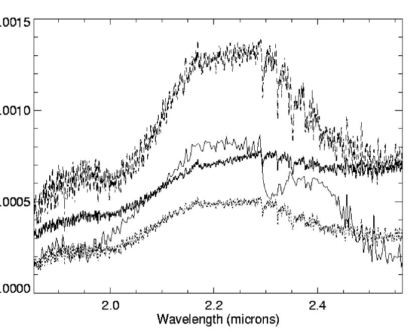
Figure 5: Comparison of contrast for the four fiducial cases. Uppermost dashed curve is the cloudless $f=2$ case. The thick middle curve is the cloudy $f=1$ case, and the lower dotted curve is the cloudless $f=1$ case; these three are the result of the simple spectral synthesis calculations, plotted at a spectral resolution of 1500. The thin, solid curve is the Sudarsky et al. (2003) baseline result for the planetary flux divided by the Kurucz model (see text).

where $T_{*}$ is the effective temperature of the star, $R_{*}$ is the stellar radius, $D$ is the orbital radius of the planet, and $A$ is the Bond albedo. The parameter $f$ quantifies the redistribution of incident stellar radiation; the $f=1$ case represents the situation in which the incident radiation is evenly redistributed over the entire planet, while the $f=2$ case represents the one in which the incident radiation is completely absorbed and re-emitted on the day side of the planet. The Sudarsky et al. (2003) baseline model assumes $f=2$ (or equivalently, $f=0.5$ using their definition of $f$ (Saumon et al., 2002)). As noted, our first case for comparing with the observational results is the baseline Sudarsky et al. (2003) flux divided by the Kurucz model. We choose three other cases as fiducial models for comparison with the data. These have been selected in order to test a wide range of the possible physical conditions in the atmosphere. We choose two $f=1$ models based on the formulation by Seager & Sasselov (1998); Seager et al. (2000), one with no clouds and one with cloud opacity due to MgSiO₃, Fe, and Al₂O₃. Since the Sudarsky et al. (2003) baseline model considers cloud opacities and assumes $f=2$, we further select a cloudless model with $f=2$ (based on the Seager & Sasselov (1998); Seager et al. (2000) formulation). The temperature profiles of these four cases are shown in Figure 4, and the results for the four flux peaks (the Sudarsky et al. (2003) baseline result as well as the cloudless and cloudy fiducial cases) are shown in Figure 5.

5 RESULTS AND INTERPRETATION

We now fit these four modeled flux peaks to the data using linear least squares, as in

$$r_{i}=a+bm_{i},$$ (8)

where $r_{i}$ represents the resulting difference spectrum (e.g., Figure 3), $m_{i}$ represents the contrast ratio from a given model, $i$ represents the wavelength bin, and $a$ and $b$ are the coefficients of the fit. The slope of this fit, $b$, which we call the ‘model amplitude,’ therefore represents the ‘amount’ of the model signal that appears in the data. A model amplitude of unity would mean that the model clearly fits the data (depending on the errors), while a value of zero represents no correlation between the model and the data. Note that the $y$-offset between the model and the data is irrelevant, since we are searching only for the evidence of the shape of a given model within the data. The results for the four fiducial models are shown in Table 1. For each model, we indicate the model amplitude $b$, the uncertainty in $b$, and the reduced chi-squared of the fit. We further list the reduced chi-squared for the case in which we force the model amplitude to be unity; that is, we assume that the model appears in the data at full strength. For all four fiducial models, the slope of the fit is roughly zero, suggesting that none of them fit the data. However, the rejection is much stronger for the both $f=2$ models, as seen by the reduced chi-squared values for forcing the model amplitude to be unity. These high values indicate that it is extremely unlikely that the $f=2$ models fit the data. Given that the observations and analysis are highly differential, we are furthermore confident that a peak in the planetary spectrum is not being fortuitously canceled by some systematic error in the data.

The least squares fit described above is difficult to interpret for models with small amplitude flux peaks, as in some of our scaled models (see Equations 3 and 4). It is also desirable to explore another way to quantify the degree to which the four specific models are rejected by the data. We use a Monte Carlo technique to accomplish this. To quantify the statistical significance of the rejection of any particular model, we constructed ‘fake data’ by adding normally-distributed noise to the modeled contrast values, with $\sigma$ equal to the size of the error bar in each bin of Figure 3. We created 10⁵ fake data sets for each model and then fit each one to the original model using linear least squares (in the same way in which the real data were fit to the model to calculate the model amplitude). Next, we determine the number of resulting model amplitudes which are greater than the value obtained by fitting the original model to the actual data; this is a liberal criterion for concluding that the model is consistent with a given fake data set. The percentage of fake data sets consistent with a given model, using this criterion, is the ‘detection efficiency’, $Q$. A high value of $Q$, say $>99\%$, implies that a given model consistently produced at least a minimal signature in the fake data. The results for the four specific models discussed thus far are shown in Table 2, and are also plotted in Figure 6 (filled symbols). A model with a high detection efficiency using the Monte Carlo technique implies that it is detectable. Thus, the two $f=2$ models—having model amplitudes near zero and high detection efficiencies—are again concluded to be rejected. These results are consistent with the chi-squared analysis described above.

We tested our suite of scaled models, with the prescription given by Equation 3, using this technique. The parameters and results of these models, as well as the model amplitudes, are shown in Table 3 for the cloudless $f=1$ cases and in Table 4 for the cloudy $f=1$ cases. The results of $Q$ vs. $\Delta T$ are plotted in Figure 6 for both sets of models. We reject a model if it has a value of $Q>99\%$ and also has a model amplitude near zero. Looking at Tables 3 and 4, the rejected models correspond to the steeper T/P profiles, with $\gamma\geq 1.25$. Thus, we can see that the temperature profiles with a higher temperature gradient, causing a larger peak near 2.2 µm in the emergent spectrum, can be eliminated as inconsistent with our observations. The more isothermal profiles, on the other hand, are consistent with the data. Figure 6 suggests that only models with $\Delta T\lesssim 1100$ K are consistent with our data. Although the rejection limit also depends on $T_{\mbox{\scriptsize{offset}}}$ from Equation 3, it is strongly dependent on $\Delta T$.

6 CONCLUSION

Our results are extremely sensitive to the temperature-pressure profile, which is as expected, given that the Planck function varies strongly with temperature in this wavelength region. Besides the shape of the profile, there are a variety of other possible processes in the planetary atmosphere that could render the planet undetectable with these observations. For example, the broad peak in the spectrum near 2.2 µm is caused by the large number of weak water lines on either side of this feature. Absorption by these lines lowers the continuum level on either side, thus creating the peak. One obvious process by which the peak would not appear is a lowering of the water abundance in the planetary atmosphere. We tested this idea and found that only when the water abundance was lowered by a factor of 10 did the peak become small enough to escape detection using our method. This value for the water abundance ($\sim 9.8\times 10^{-5}$) seems unrealistically small.

We suggest three ways in which the 2.2 µm flux peak would be lowered sufficiently to be consistent with our observations. The first is the efficient redistribution of the incident radiation over the entire planet, which can be achieved through atmospheric dynamics, i.e., winds. Depending on how efficiently the incident radiation is redistributed, the effect could be a temperature asymmetry between the ‘day’ and ‘night’ sides of the planet. Showman & Guillot (2002) suggest that the day-night temperature difference may be as much as 300 K; even a difference of this magnitude would lead to strong winds of 1 km s^-1 or more. The $f=2$ situation would tend to steepen the T/P profile in the atmosphere, since the strong stellar irradiation would have to be absorbed relatively deep in the atmosphere and re-radiated. The two specific $f=2$ models considered above, which assume that the heat is absorbed and re-radiated only on the day side, are inconsistent with our data (as shown in Table 1). This suggests that the large temperature asymmetry scenario may not be viable and that some sort of transport mechanism may be at work to move the incident energy from the hot to the cold side. We caution that we have observed only two secondary eclipses of HD 209458 b; recent simulations by Cho et al. (2003) indicate that the temperature asymmetry between the two hemispheres may be time-variable. This effect can be so strong as to render the day side to be colder than the night side at times.

A second mechanism by which the 2.2 µm flux peak could be lowered is additional opacity in the upper atmosphere, which would flatten the T/P profile and thus reduce the relative strength of the peak. For example, the T/P profiles shown by Barman et al. (2001) are nearly isothermal, and will certainly produce 2 µm spectra consistent with our observed limit. Barman (2003, private communication) attributes this behavior to their treatment of the opacity, specifically the inclusion of strong gaseous opacity due to metals, which differs from the opacity treatment in other models. However, consistency with our data does not necessarily indicate that a given model is correct, and we leave it to the theorists to sort out the differences among competing models. We suggest that a high-altitude cloud (first suggested by Seager & Sasselov (2000) and favored by Charbonneau et al. (2002) to explain their low sodium result) would also make the atmosphere more isothermal if the cloud is sufficiently absorbing and vertically extended. Note, however, that the Charbonneau et al. (2002) sodium result requires placing such a cloud at the limb of the planet, whereas our results require the clouds to be broadly distributed on the day side.

A high cloud might also affect the emergent spectrum through a third mechanism. For a sufficiently high cloud, the atmosphere above the cloud deck would be thin, giving a small column density in which a spectral signature could be formed. Very little incident radiation would penetrate an optically thick cloud, meaning that the temperature structure would be dominated by the blackbody reflection or emission of the cloud itself. The emergent spectrum would be determined by the small part of the atmosphere above the cloud deck, rather than the details of the T/P profile.

Finally, we note that our results have been obtained using the 3-meter IRTF, indicating that valuable observations of extrasolar planets, leading to new information on the atmospheres of these objects, can be conducted using modest-aperture telescopes from the ground, given favorable observing conditions and careful analysis.

Table 1: Results of the least squares fit of the data to each of the four fiducial models, indicating the slope (model amplitude) $b$ and the uncertainty in $b$, as well as the reduced chi-squared for the fit. The rightmost column indicates the reduced chi-squared value for the case in which we force the slope to be unity.

Model	$b$	$\sigma_{b}$	$\bar{\chi}^{2}$	$\bar{\chi}^{2}(b=1)$
Cloudless (f=1)	0.02	$\pm$ 0.29	2.35	2.85
Cloudless (f=2)	0.03	$\pm$ 0.10	2.34	6.43
Cloudy (f=1)	-0.25	$\pm$ 0.24	2.30	3.43
Cloudy (f=2)	-0.01	$\pm$ 0.14	2.35	4.66

Table 2: Results from the Monte Carlo technique for the four fiducial models. The value of $\Delta$T from Equation 4 is shown, as well as the value $Q$ describing the efficiency of the detection using the Monte Carlo technique, as plotted in Figure 6.

Model	$\Delta$T (K)	Q (%)
Cloudless (f=1)	960.36	99.3
Cloudless (f=2)	1265.38	100.0
Cloudy (f=1)	797.92	100.0
Cloudy (f=2)	$\sim$ 1180	100.0

Table 3: Results for scaled cloudless $f=1$ profiles. The first column is the value of $\Delta T$ from Equation 4, and the scaling parameters are defined in Equation 3. The model amplitude $b$ and uncertainty $\sigma_{b}$ are also shown. The value $Q$ represents the detection efficiency using the Monte Carlo technique, as plotted in Figure 6 (diamonds).

$\Delta$T (K)	$\gamma$	T${}_{\mbox{offset}}$	b	$\sigma_{b}$	Q (%)
517.42	0.50	0	-1.49	1.35	89.7
510.21	0.50	100	-0.78	0.81	93.4
510.00	0.50	-100	-1.84	2.05	81.9
750.58	0.75	0	-0.13	0.53	93.0
734.92	0.75	100	-0.13	0.40	97.5
762.85	0.75	-100	-0.16	0.75	85.7
960.36	1.00	0	0.02	0.29	99.3
939.94	1.00	100	-0.00	0.24	99.9
978.55	1.00	-100	0.05	0.36	97.1
1151.05	1.25	0	0.04	0.18	100.0
1128.48	1.25	100	0.02	0.16	100.0
1175.98	1.25	-100	0.06	0.21	99.9
1328.16	1.50	0	0.04	0.13	100.0
1300.31	1.50	100	0.03	0.11	100.0
1357.76	1.50	-100	0.05	0.14	100.0
1652.07	2.00	0	0.03	0.07	100.0
1623.06	2.00	100	0.03	0.07	100.0
1684.67	2.00	-100	0.04	0.08	100.0

Table 4: Results for the scaled cloudy $f=1$ profiles. The same quantites as described in Table 3 are shown. The values for the detection efficiency $Q$ are also plotted in Figure 6 (squares).

$\Delta$T (K)	$\gamma$	T${}_{\mbox{offset}}$	b	$\sigma_{b}$	Q (%)
418.63	0.50	0	-0.83	0.49	99.6
413.15	0.50	100	-0.65	0.38	99.9
422.91	0.50	-100	-1.14	0.65	98.9
612.63	0.75	0	-0.46	0.33	99.9
605.37	0.75	100	-0.38	0.27	100.0
620.46	0.75	-100	-0.58	0.42	99.6
797.92	1.00	0	-0.25	0.24	100.0
787.74	1.00	100	-0.22	0.20	100.0
808.55	1.00	-100	-0.30	0.28	99.9
976.03	1.25	0	-0.14	0.18	100.0
964.24	1.25	100	-0.13	0.16	100.0
987.11	1.25	-100	-0.16	0.20	100.0
1147.48	1.50	0	-0.08	0.14	100.0
1136.11	1.50	100	-0.08	0.12	100.0
1160.71	1.50	-100	-0.09	0.15	100.0
1481.52	2.00	0	-0.03	0.09	100.0
1470.01	2.00	100	-0.03	0.08	100.0
1495.06	2.00	-100	-0.03	0.10	100.0

Figure 1: Sample extracted spectra of HD 209458 (lower, thick curve) and HD 210483 (upper, thin curve) from UT 27 September (near air mass of 1.27). The comparison star has not yet been normalized for subtraction from the HD 209458 spectrum. The overall shape of the spectra is due to the instrument response function. Spectral features are primarily telluric.

Figure 2: Sample binned residual spectrum from UT 27 September, corresponding to spectra shown in Figure 1. Five different orders from the spectrograph (three in the short wavelength region (1.9–2.5 µm) and two in the long wavelength region (3.0–4.1 µm)) are shown as alternating filled and empty symbols. Because of large uncertainties resulting from the terrestrial background, the long wavelength data are not considered further in this analysis.

Figure 3: Final difference spectrum, calculated by averaging the data from the two ‘in-eclipse’ nights. This was obtained using 550 individual spectra of HD 209458, with an equal number of HD 210483 spectra. The Sudarsky et al. (2003) baseline model is over-plotted at a higher spectral resolution ($\lambda/\Delta\lambda\sim 2200$) than the binned data. The offset between the model and the data is not important, since we are comparing the shapes of the two spectra; thus, the mean has been subtracted from the data and model, respectively, for plotting purposes.

Figure 4: Temperature-pressure profiles of the four fiducial cases. The dashed curve is from the Sudarsky et al. (2003) baseline model, the thick solid curve is the cloudy $f=1$ case, the thin lower curve is the cloudless $f=1$ case, and the dotted line is the cloudless $f=2$ case.

Figure 6: Detection efficiency $Q$ for a suite of scaled models vs. $\Delta T$, which represents the difference between the temperature at optical depth unity at the center of the bandpass and the boundary temperature (see Equation 4). See Tables 3 and 4 for details of each scaled profile. The filled symbols, along with the asterisk, represent the four fiducial cases described in Table 2.

References

- Barman et al. (2001) Barman, T. S., Hauschildt, P. H., & Allard, F. 2001, ApJ, 556, 885
- Borysow (2002) Borysow, A. 2002, A&A, 390, 779
- Brown et al. (2001) Brown, T. M., Charbonneau, D., Gilliland, R. L., Noyes, R. W., & Burrows, A. 2001, ApJ, 552, 699
- Burrows & Sharp (1999) Burrows, A. & Sharp, C. M. 1999, ApJ, 512, 843
- Charbonneau (2003) Charbonneau, D. 2003, in ASP Conference Series, Scientific Frontiers in Research on Extrasolar Planets, D. Deming and S. Seager; Eds., Vol. 294, 449
- Charbonneau et al. (2000) Charbonneau, D., Brown, T. M., Latham, D. W., & Mayor, M. 2000, ApJ, 529, L45
- Charbonneau et al. (2002) Charbonneau, D., Brown, T. M., Noyes, R. W., & Gilliland, R. L. 2002, ApJ, 568, 377
- Cho et al. (2003) Cho, J. Y.-K., Menou, K., Hansen, B. M. S., & Seager, S. 2003, in ASP Conference Series, Scientific Frontiers in Research on Extrasolar Planets, D. Deming and S. Seager; Eds.
- Cody & Sasselov (2002) Cody, A. M. & Sasselov, D. D. 2002, ApJ, 569, 451
- Goorvitch (1994) Goorvitch, D. 1994, ApJS, 95, 535
- Guillot et al. (1996) Guillot, T., Burrows, A., Hubbard, W. B., Lunine, J. I., & Saumon, D. 1996, ApJ, 459, L35+
- Henry et al. (2000) Henry, G. W., Marcy, G. W., Butler, R. P., & Vogt, S. S. 2000, ApJ, 529, L41
- Jørgensen et al. (2000) Jørgensen, U. G., Hammer, D., Borysow, A., & Falkesgaard, J. 2000, A&A, 361, 283
- Kenworthy & Hinz (2003) Kenworthy, M. A. & Hinz, P. M. 2003, PASP, 115, 322
- Kurucz (1992) Kurucz, R. L. 1992, in IAU Symp. 149: The Stellar Populations of Galaxies, 225–+
- Linfield et al. (2001) Linfield, R. P., Colavita, M. M., & Lane, B. F. 2001, ApJ, 554, 505
- Lucas & Roche (2002) Lucas, P. W. & Roche, P. F. 2002, MNRAS, 336, 637
- Mazeh et al. (2000) Mazeh, T., Naef, D., Torres, G., Latham, D. W., Mayor, M., Beuzit, J., Brown, T. M., Buchhave, L., Burnet, M., Carney, B. W., Charbonneau, D., Drukier, G. A., Laird, J. B., Pepe, F., Perrier, C., Queloz, D., Santos, N. C., Sivan, J., Udry, S. ., & Zucker, S. 2000, ApJ, 532, L55
- Nidever et al. (2002) Nidever, D. L., Marcy, G. W., Butler, R. P., Fischer, D. A., & Vogt, S. S. 2002, ApJS, 141, 503
- Partridge & Schwenke (1997) Partridge, H. & Schwenke, D. W. 1997, J. Chem. Phys., 106, 4618
- Rayner et al. (2003) Rayner, J. T., Toomey, D. W., Onaka, P. M., Denault, A. J., Stahlberger, W. E., Vacca, W. D., Cushing, M. C., & Wang, S. 2003, PASP, 115, 362
- Richardson et al. (2003) Richardson, L. J., Deming, D., Wiedemann, G., Goukenleuque, C., Steyert, D., Harrington, J., & Esposito, L. W. 2003, ApJ, 584, 1053
- Rothman et al. (1998) Rothman, L. S., Rinsland, C. P., Goldman, A., Massie, S. T., Edwards, D. P., Flaud, J.-M., Perrin, A., Camy-Peyret, C., Dana, V., Mandin, J.-Y., Schroeder, J., McCann, A., Gamanche, R. R., Wattson, R. B., Yoshino, K., Chance, K., Jucks, K., Brown, L. R., Nemtchinov, V., & Varanasi, P. 1998, Journal of Quantitative Spectroscopy and Radiative Transfer, 60, 665
- Saumon et al. (2002) Saumon, D., Marley, M. S., Lodders, K., & Freedman, R. S. 2002, ArXiv Astrophysics e-prints, 7070
- Schultz et al. (2003) Schultz, A. B., Kochte, M., Kinzel, W., Hamilton, F., & Jordan, I. 2003, in ASP Conference Series, Scientific Frontiers in Research on Extrasolar Planets, D. Deming and S. Seager; Eds., Vol. 294, 479
- Seager & Sasselov (1998) Seager, S. & Sasselov, D. D. 1998, ApJ, 502, L157
- Seager & Sasselov (2000) —. 2000, ApJ, 537, 916
- Seager et al. (2000) Seager, S., Whitney, B. A., & Sasselov, D. D. 2000, ApJ, 540, 504
- Showman & Guillot (2002) Showman, A. P. & Guillot, T. 2002, A&A, 385, 166
- Sudarsky et al. (2003) Sudarsky, D., Burrows, A., & Hubeny, I. 2003, ApJ, 588, 1121
- Vacca et al. (2003) Vacca, W. D., Cushing, M. C., & Rayner, J. T. 2003, PASP, 115, 389
- Wilson (1953) Wilson, R. E. 1953, Carnegie Institute Washington D.C. Publication, 0
- Wittenmyer et al. (2002) Wittenmyer, R. A., Welsh, W. F., & Orosz, J. A. 2002, American Astronomical Society Meeting, 201, 0