RR Lyrae stars in four globular clusters in the Fornax dwarf galaxy
Abstract
We have surveyed four of the globular clusters in the Fornax dwarf galaxy (clusters 1, 2, 3, and 5) for RR Lyrae stars, using archival F555W and F814W Hubble Space Telescope observations. We identify 197 new RR Lyrae stars in these four clusters, and 13 additional candidate horizontal branch variable stars. Although somewhat restricted by our short observational baseline, we derive periods and light-curves for all of the stars in the sample, and calculate photometric parameters such as mean magnitudes and colours. This is the first time that RR Lyrae stars in the Fornax globular clusters have been quantitatively identified and measured. We find that the Fornax clusters have exceptionally large specific frequencies of RR Lyrae stars, in comparison with the galactic globular clusters. It is likely that Fornax 1 has the largest specific frequency measured in any globular cluster. In addition, the Fornax clusters are unusual in that their RR Lyrae populations possess mean characteristics intermediate between the two Oosterhoff groups defined by the galactic globular clusters. In this respect the RR Lyrae populations in the Fornax clusters most closely resemble the field populations in several dwarf galaxies. Fornax 5 has an unusually large fraction of RRc stars, and also possesses several strong RRe (second overtone pulsator) candidates.
With a large sample of horizontal branch variable stars available to us, we revise previous measurements of the horizontal branch morphology in each cluster. The Fornax clusters most closely resemble the “young” galactic halo population defined by Zinn in that their horizontal branch morphologies are systematically redder than many galactic clusters of similar metallicity. We also confirm the existence of the second parameter effect among the Fornax clusters, most markedly between clusters 1 and 3. The edges of the instability strip are well defined in several of the Fornax clusters, and we are able to make measurements of the intrinsic colours of these edges. Finally, we determine foreground reddening and distance estimates for each cluster. We find a mean distance modulus to the Fornax dwarf of (random) (systematic). Our measurements are consistent with a line of sight depth of kpc for this galaxy, which is in accordance with its dimensions as measured in the plane of the sky. This approximately spherical shape for Fornax is incompatible with tidal model explanations for the observed high internal stellar velocity dispersions in many dwarf spheroidal galaxies. Dark matter dominance is suggested.
keywords:
stars: variables: other – stars: horizontal branch – galaxies: star clusters – globular clusters: general – galaxies: individual: Fornax dwarf spheroidal1 Introduction
The Fornax dwarf galaxy is one of the most massive of the dwarf spheroidal (dSph) galaxies associated with the Milky Way (second only to the disrupted Sagittarius dSph), and the only undisturbed local galaxy to possess globular clusters (although Kleyna et al. [2003] have recently suggested the presence of a disrupted cluster in the Ursa Minor dSph). In this respect Fornax is somewhat unusual, because its population of five means that it has the highest specific frequency of globular clusters for any known galaxy.
As summarized by Strader et al. [2003], although small in number, this globular cluster system is remarkably complex. Buonanno et al. [1998b, 1999] have shown that clusters 1, 2, 3, and 5 appear coeval with both each other and the metal-poor galactic globular clusters, and that cluster 4 may be up to three gigayears younger. Strader et al. [2003] suggest that Fornax 5 may also be slightly younger. It has also been found [1996, 1998b] that the Fornax globular clusters show evidence of the second parameter effect, whereby another parameter in addition to metallicity appears to define the morphology of the horizontal branch in a cluster. It is often assumed that age is the second parameter; however, if the age measurements listed above are correct, then it is possible that age is not the sole second parameter in the Fornax clusters. We [2003b] have studied the surface brightness profiles of the Fornax globular clusters, and find a large amount of variation in the cluster structures – ranging from an extremely extended cluster (Fornax 1), to a strong post core-collapse candidate (Fornax 5). Evidently the Fornax cluster system is highly complicated; however both this complexity, and the system’s isolated nature provide unique opportunities for addressing the outstanding difficulties in our understanding of globular cluster formation and evolution. The Fornax globular clusters are therefore worthy of detailed study.
Much can be learned about a stellar population from the variable stars within that population, and given the relatively close proximity of the Fornax dwarf, it is perhaps surprising that a detailed investigation of stellar variability in its clusters has not been undertaken. In fact, we can find no quantitative identification and measurements of any variable stars in these objects in the literature – only several passing mentions of possible RR Lyrae detections exist [1985, 1990, 1996, 1996, 1997, 1998b], along with one short article describing a survey in progress, and including cluster 3 [2003].
In the process of obtaining photometry for colour-magnitude diagrams from archival Hubble Space Telescope observations, we noticed the possibility of surveying four of the Fornax globular clusters for RR Lyrae stars. We present here the results of this survey, which has been successful beyond our original expectations. We have discovered 197 RR Lyrae stars in the four clusters (Fornax 1, 2, 3, and 5), as well as 13 candidate horizontal branch variables. We describe the data and our survey strategy in Section 2, and present light curves and mean properties for each star in Section 3. Finally, we have been able to use the RR Lyrae discoveries to measure detailed information about each of the four clusters under consideration. This discussion is presented in Section 4.
2 Observations and Reductions
2.1 Data
| Cluster | Data-group | Reference | Baseline | Exposure | Data-group | Exposure | ||
|---|---|---|---|---|---|---|---|---|
| Name | F555W | Image | (days) | Durations (s) | F814W | Durations (s) | ||
| Fornax 1 | u30m010eb | u30m010et | 0.3595 | 14 | 3600s, 4500s, | u30m010ib | 16 | 2900s, 6700s, |
| 3400s, 4160s | 2500s, 6120s | |||||||
| Fornax 2 | u30m020eb | u30m020et | 0.3602 | 14 | 3600s, 4500s, | u30m020ib | 16 | 2900s, 6700s, |
| 3400s, 4160s | 2500s, 6120s | |||||||
| Fornax 3 | u30m030eb | u30m030et | 0.3602 | 14 | 3600s, 3500s, 3400s, | u30m030ib | 16 | 2900s, 6700s, |
| 1378s, 4160s | 2500s, 6120s | |||||||
| Fornax 5 | u30m040eb | u30m040et | 0.3553 | 14 | 3600s, 4500s, | u30m040ib | 16 | 2900s, 6700s, |
| 3400s, 4160s | 2500s, 6120s |
Wide Field Planetary Camera 2 (WFPC2) observations of four of the globular clusters in the Fornax dwarf galaxy (clusters 1, 2, 3, and 5, according to the notation of Hodge [1961]) are available in the HST archive (Program ID 5917). These observations were made between 1996 June 4 and 1996 June 6, through the F555W and F814W filters. The observational details are listed in Table LABEL:observations.
Each cluster was imaged 14 times in F555W and 16 times in F814W, with individual exposure durations ranging from s, and s, respectively. Long total integration times are necessary because of the faintness of the Fornax globular clusters, which have distance moduli [1999]. The image sampling, presumably primarily intended to facilitate the removal of cosmic rays over the long integrations, renders the data suitable for identifying sources with short period variability, such as RR Lyrae stars. The exposure durations complement such identification, with horizontal branch (HB) stars being among the brightest stars in each image, and neither saturated nor overly faint in any image. Furthermore, observations through the two filters are interleaved, so that for any given F555W observation, it is possible to find an F814W image with a similar exposure duration and an observation date matching to days. Such pairing of images allows colour information over a star’s variability cycle to be measured.
Although otherwise well suited for an RR Lyrae star search, the data have very short baselines of observation. This means that while variability can be easily detected, period determination is not straightforward – especially for RRab type variables, which typically have periods in the range days. Unless such stars are fortuitously measured at a critical region of their light curve, the under-sampling renders accurate period determination virtually impossible. The shorter cycle RRc type variables, which have periods of days, are more suited to the observation baselines. We will return to the question of period determination in Section 2.4.
Finally, we note that there also exist archival WFPC2 observations of Fornax cluster 4 (Program ID 5637). However, the data consist of only three images per filter, and given the significant crowding and field star contamination for this cluster, were not suitable for the present RR Lyrae work. We do not consider Fornax 4 further.
2.2 Photometry
All WFPC2 images we retrieved from the HST archive underwent preliminary reduction according to a standard pipeline, using the latest available calibrations. For photometric measurements from these calibrated images we used Dolphin’s HSTphot [2000a]. This is a photometric package specifically designed for use on WFPC2 data. In particular, it uses a library of point spread functions (PSFs) tailored to account for the undersampled WFPC2 PSFs, allowing very accurate stellar centroiding and photometry.
Before running HSTphot, we completed several preprocessing steps. For each cluster, a reference image was identified (these are listed in Table LABEL:observations) and all other images aligned with this image. This was achieved using the iraf task imalign, treating each image offset as a simple - and -shift. This is perfectly adequate for the present data – each image for a given cluster is offset from the reference image due to a simple dithering pattern of several pixels. There are no significant higher order distortions to account for.
Next, we used the utility software accompanying HSTphot to mask image defects (such as bad pixels and columns), calculate a background sky image (for use in the photometry calculations), and attempt to remove cosmic rays and unmasked hot-pixels. We then made photometric measurements on each image using HSTphot in PSF fitting mode (as opposed to aperture photometry mode). We set a minimum threshold for object detection of above the background. We also enabled two additional features of HSTphot. First, we elected to calculate a local adjustment to the background image before each photometry measurement, using the pixels just beyond the photometry radius [2000a]. This helped account for regions of rapidly varying background, such as near the centres of the very crowded clusters 3 and 5. Second, we chose to run artificial star tests in conjunction with the photometry measurements. This option generates a large number of “fake” stars on a CMD, places them one at a time on the image, and solves each just as if it were a real star. This allows quantitative estimates of detection completeness as a function of a star’s magnitude, colour, and position in a cluster.
For each photometric measurement of a star (ideally, 14F555W measurements and 16F814W measurements) HSTphot output nine parameters, including flight magnitudes, standard magnitudes, and quantities characterizing the goodness-of-fit of the PSF solution (e.g., classification type, , S/N, and sharpness). Magnitudes from HSTphot are calibrated according to the recipe of Holtzman et al. [1995], and using the latest updates of the Dolphin [2000b] CTE and zero-point calibrations. Each magnitude is corrected to a aperture. HSTphot also provided mean positional information for each object, in the form of a chip number (where chip refers to the PC, and chips to WFC2-WFC4 respectively) and pixel coordinates relative to the frame of the reference image. These coordinates, in conjunction with the iraf task metric and the cluster centres measured in Mackey & Gilmore [2003b], allowed us to calculate the radial distance of a given object from the centre of its cluster.
We used the goodness-of-fit parameters to select only objects with high quality photometry. We retained only measurements for which an object was classified as stellar (HSTphot types 1, 2, and 3), and for which , S/N , sharpness , and errors in the flight magnitude . After the application of this filter, we kept only stars with five or more F555W-F814W pairs of successful measurements (where a pair is defined as two observations within days of each other, as described in Section 2.1). We also passed the artificial star measurements through the quality filter. This allowed us to assign a detection completeness to each real star, by finding the fraction of successful artificial star measurements in a brightness-colour-position bin about the real star. Bin widths were mag in brightness, mag in colour, and in radial distance from the cluster centre. As an example, we consider a typical Fornax globular cluster RR Lyrae star, of magnitude , colour , and radial distance . The fraction of successful artificial star measurements with , , and defines the detection completeness for this star. We expect the completeness values so derived to be accurate to a few per cent, except for very low fractions. Values of less than should be regarded with caution.
2.3 Identification of Horizontal Branch variable stars
The completion of the photometry procedure resulted in a list of stars in each cluster, each with between 5 and 14 pairs of F555W and F814W measurements. In general, most stars possessed measurement pairs. Using colour-magnitude diagrams (CMDs) we selected stars in the HB region of each cluster, and determined the Welch & Stetson [1993] variability index for each. This index is calculated as follows. For epochs of observations, each resulting in measurements and , the weighted mean magnitudes
| (1) |
may be computed. The variability index is then defined as:
| (2) |
where the normalized magnitude residuals are
| (3) |
The variability index therefore allows one to preferentially search for variations in photometric measurements which are correlated in the two colours being measured. For example, an RR Lyrae star will brighten and fade in both and , in synchronization over its pulsation cycle. Variability such as this results in a large value for . In the case of random errors – for example where one or more stellar images has been impacted by a cosmic ray, causing spurious variability in one colour band, or in the case where crowding introduces large random errors into each measurement – then and are uncorrelated, and the expectation value of is zero.

We therefore selected stars for which was greater than some positive constant as candidate variables. A small amount of experimentation showed to be a suitable value. The resultant candidate variable stars are shown in Fig. 1. We identified 283 candidates in total (24, 56, 137, and 66, in clusters 1, 2, 3, and 5, respectively). In each of the HB regions on the CMDs, the RR Lyrae strip is evident, and in most cases clearly defined on both edges. For each cluster, there also in general exist some candidate variable stars in the blue HB (BHB) region (except Fornax 1, for which no BHB extension is observed), and some along the red giant branch (RGB). Because we did not want to assume any information, a priori, about the exact limits of the instability strip on the HB, we tested all flagged variable stars equally as RR Lyrae candidates.
2.4 Light-curve fitting
The best way to identify a candidate star as an RR Lyrae, and in addition obtain quantitative information about its variability parameters, is to attempt to fit a light curve to its photometry. For very under-sampled data, such as the present measurements, this can be tricky. Eschewing elegance, the most reliable method is the simple application of brute force. We used a routine written by Andrew Layden (described in Layden & Sarajedini [2000]; Layden et al. [1999]; Layden [1998]; and the references therein) for our period measurements.
This program works by taking a set of 10 variable star templates and attempting to fit them to the -band photometric measurements for a number of different periods. The periods are selected by an incremental increase over a range to . For each candidate period, the measurements are folded, and a 3-parameter fit (magnitude zero-point, phase zero-point, and light-curve amplitude) made to each template. Six of the ten templates represent RRab type variable stars, while two represent RRc type pulsators, and two represent variable binary stars (a W Ursae Majoris contact binary, and an Algol eclipsing binary). The RRab curves (templates ), and one of the RRc curves (template ) are derived from high quality measured light curves, as described in Layden & Sarajedini [2000], and Layden [1998]. The second RRc template (number 8) is a simple cosine curve. From each template fit, is calculated. Period-template combinations with small are likely to be the best representations of the measured data.
Such a procedure works well when the sampling is spread over a much longer baseline than the period of the variable star under consideration. In the present case however, our day baseline is in general less than one RR Lyrae pulsation cycle. For the short period (RRc) variables, which typically have days, this does not pose too much of a problem. It is possible to derive a reliable period estimate for these stars, although naturally, accuracy would be greatly increased by having a baseline of many periods.
The situation is not so good for the RRab variables, which might have periods typically about twice that of our baseline. It is possible to determine a reliable period estimate for such stars, but only under certain circumstances. Specifically, it is necessary to observe the full amplitude of a star’s variability (this allows the three parameters in a template fit to be well determined) and some portion of its decline from maximum (which allows discrimination between different potential periods). For a mean RRab period of days (in which case our baseline is ), examination of Figure 1 in Layden [1998] shows that we would observe the appropriate portion of the light curve in approximately per cent of cases. For shorter period RRab stars this fraction is greater, and for longer period stars it is smaller. Another per cent of the time, we might observe most of the portion of the cycle which we require, in which case the derived period will be a good estimate. In the remainder of cases, without assuming some prior knowledge of either the star’s period or its amplitude, we cannot make an accurate period determination. In these incidences, we must make do with setting a lower limit to the period, which we achieve by assuming that the observed amplitude is the real amplitude of the star. The presence of these lower limits in our period measurements must be borne in mind if the data is put to any interpretive uses (see e.g., Section 4). Measurements at future epochs are required to pin down accurately the periods of such stars.
Since we were searching for RR Lyrae stars, we chose a period range of days, with per cent. For each candidate, we examined the few fits to the -band photometry with the smallest . We used the -band data as a consistency check, to verify that a fit which appeared suitable for the -band photometry also resulted in a good -band light-curve. In general the -band data was of significantly poorer quality than the -band data, so fitting templates directly to these measurements did not add useful information to the procedure. In the vast majority of cases, the -band solution with the very smallest provided evidently the best fit. We conservatively estimate the typical random uncertainty in any of our fitted periods to be days. While we identified plenty of RR Lyrae stars, we did not find any stars with data clearly best fit by either of the variable binary star templates. However, given our restriction to a small portion of the CMD, and our very short observation baseline, this is not too surprising. Most of the candidate variables flagged on the BHB or RGB seemed to have either poor measurements or some form of irregular variability. Certainly none had values of as large as those for typical RR Lyrae stars.
3 Results
![[Uncaptioned image]](/html/astro-ph/0307275/assets/x2.png)
![[Uncaptioned image]](/html/astro-ph/0307275/assets/x3.png)
![[Uncaptioned image]](/html/astro-ph/0307275/assets/x4.png)
![[Uncaptioned image]](/html/astro-ph/0307275/assets/x5.png)
![[Uncaptioned image]](/html/astro-ph/0307275/assets/x6.png)
![[Uncaptioned image]](/html/astro-ph/0307275/assets/x7.png)
![[Uncaptioned image]](/html/astro-ph/0307275/assets/x8.png)
![[Uncaptioned image]](/html/astro-ph/0307275/assets/x9.png)
![[Uncaptioned image]](/html/astro-ph/0307275/assets/x10.png)
![[Uncaptioned image]](/html/astro-ph/0307275/assets/x11.png)
![[Uncaptioned image]](/html/astro-ph/0307275/assets/x12.png)
![[Uncaptioned image]](/html/astro-ph/0307275/assets/x13.png)


3.1 RR Lyrae stars
Of the 283 candidate objects, we identified 197 as RR Lyrae stars (15, 43, 99, and 40, in clusters 1, 2, 3, and 5, respectively). For each of these stars, we obtained template fits and period measurements. The best fitting -band light curves are presented in Fig. 2, and the positions, periods, and fit parameters (template, rms scatter) listed in Table 2. In this table, the coordinates (chip, , ) are relative to the reference images listed in Table LABEL:observations, and are in units of pixels. “Chip” refers to the camera on which the star was imaged – is the PC, and are WFC2–WFC4. The radii () and completeness fractions () are calculated as described in Section 2.2. refers to the label of the best fitting template – numbers are RRab templates, and are RRc templates. We consider periods marked with a star to be lower limit measurements. Note that on average, per cent of RRab stars have periods which are not lower limits – in accordance with our estimate in Section 2.4. In addition, we have marked several stars with question marks next to their type. In these cases, the light curves were best fit by a template of the RR Lyrae type listed (i.e., RRab or RRc), but could be fit by a template of the other RR Lyrae type almost equally as well. Further measurements are required to confirm the listed classification for these stars.
It is clear from the values that the only regions significantly affected by detection incompleteness are the very centres of the very crowded clusters 3 and 5. For cluster 3, completeness is significantly degraded within , and there are only two detections within . Cluster 5 appears even more compact (cf. Mackey & Gilmore [2003b]), with completeness only degraded within ; however, we note that there is only one detection within .
From the best fitting light curves, we computed an intensity mean magnitude, denoted , and the maximum, minimum, and amplitude of the variability (, , and , respectively). We note that these quantities are in general not significantly different from the same parameters derived directly from the -band measurements. From the -band measurements, we calculated the intensity mean . is the number of pairs of observations for a given star. The parameter is the epoch of maximum, in days since MJD . The reader should bear in mind that this parameter is derived using a star’s measured period. These quantities are all listed in Table 2.
We also characterized the colour of each RR Lyrae star. In accordance with Sandage [1990, 1993], we have calculated the magnitude mean of the measurements per RR Lyrae to best represent the colour of an “equivalent static star”. This quantity, , is in preference to the two possible intensity mean colours and . Finally, the magnitude mean colour of an RR Lyrae star at its minimum light (defined to be phases ) can be of use (see Section 4.4). For stars with measurements falling in this phase range, we also calculated this colour (denoted ). Both colours are listed in Table 2, together with the calculated error in , and the number of observations at minimum light used in its calculation.
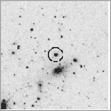
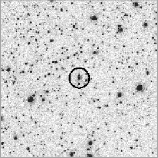
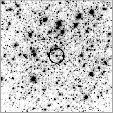
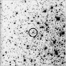
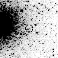
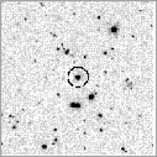
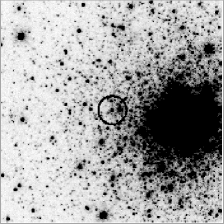
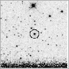
Finally, using the coordinates listed in Table 2, we constructed a finder chart for each RR Lyrae star. For reasons of practicality, we have not included the full set of charts in this paper; however, some examples are displayed in Fig. 3. The remainder are available from the author on request. Alternatively, they may be downloaded from http://www.ast.cam.ac.uk/STELLARPOPS/Fornax_RRLyr/ along with the light-curves, and data from Table 2.
Table 2: Measured and calculated properties of the RR Lyrae stars. Name Chip Period Type rms (pix) (pix) (days) F1V01 1 206.81 310.88 43.50 1.00 0.459 RRc 7 0.016 21.275 20.822 0.452 14 21.034 21.516 0.482 237.4963 0.489 0.034 4 F1V02 1 383.22 130.61 29.80 1.00 0.570 RRab 3 0.030 21.206 20.687 0.492 14 20.765 21.460 0.695 237.8765 0.652 0.025 1 F1V03 3 118.48 282.34 26.11 1.00 0.425 RRc 7 0.015 21.261 20.798 0.450 14 21.055 21.465 0.410 237.4490 0.512 0.021 2 F1V04 3 209.32 86.92 35.78 1.00 0.396 RRc 7 0.017 21.281 20.794 0.495 14 21.054 21.508 0.454 237.6898 0.582 0.016 3 F1V05 1 410.36 122.48 30.62 1.00 0.589 RRab 2 0.026 21.285 20.697 0.503 13 20.842 21.599 0.757 237.2573 0.652 0.027 1 F1V06 0 464.51 285.29 8.00 1.00 0.440 RRc 7 0.026 21.169 20.691 0.483 14 20.939 21.399 0.460 237.6960 0.500 0.015 4 F1V07 0 586.78 766.38 17.53 1.00 0.580 RRab 3 0.039 21.348 20.690 0.576 14 20.775 21.693 0.918 237.2618 0.738 0.032 2 F1V08 0 709.54 616.83 16.99 1.00 0.465∗ RRab 6 0.034 21.195 20.756 0.496 14 20.687 21.604 0.917 237.7498 0.598 0.017 4 F1V09 0 402.46 183.91 11.64 1.00 0.436 RRc 7 0.023 21.293 20.748 0.555 14 21.104 21.477 0.373 237.5112 0.569 0.040 4 F1V10 0 362.44 160.38 12.68 1.00 0.670 RRab 5 0.032 21.299 20.786 0.641 14 20.710 21.667 0.957 237.4937 0.715 0.018 5 F1V11 1 242.83 101.56 22.72 1.00 0.503∗ RRab 3 0.011 21.228 20.716 0.562 14 20.777 21.488 0.711 237.7337 0.654 0.014 4 F1V12 0 587.09 652.50 13.52 1.00 0.644 RRab 2 0.019 21.287 20.619 0.664 13 20.940 21.525 0.585 237.4082 0.733 0.020 6 F1V13 3 132.83 53.26 30.19 1.00 0.424∗ RRab? 1 0.012 21.290 20.673 0.592 14 21.002 21.442 0.440 237.4022 0.638 0.021 4 F1V14 0 379.05 321.76 5.34 1.00 0.460∗ RRab 6 0.032 21.307 20.735 0.606 14 20.806 21.710 0.904 237.7688 0.704 0.016 4 F1V15 0 736.93 535.03 16.79 0.98 0.556∗ RRab 4 0.022 21.444 20.802 0.700 14 21.147 21.659 0.512 237.6896 0.706 0.016 4 F2V01 0 386.68 480.06 2.25 0.96 0.429∗ RRab 4 0.019 21.223 20.786 0.469 14 20.626 21.701 1.075 239.5524 0.620 0.021 6 F2V02 0 538.01 546.13 9.66 0.98 0.578 RRab 2 0.024 21.315 20.890 0.560 14 20.698 21.778 1.08 239.6668 0.662 0.015 6 F2V03 0 282.08 409.83 3.52 0.96 0.375 RRc 8 0.021 21.209 20.786 0.418 14 20.962 21.488 0.526 239.8160 0.411 0.016 4 F2V04 0 368.29 260.99 8.50 1.00 0.335 RRc 7 0.021 21.258 20.926 0.389 14 20.971 21.552 0.581 239.7316 0.479 0.017 4 F2V05 0 617.42 580.55 13.57 0.97 0.664 RRab 5 0.024 21.237 20.715 0.542 14 20.795 21.498 0.703 239.4942 0.610 0.017 8 F2V06 3 141.64 576.57 47.35 1.00 0.336 RRc 7 0.009 21.455 20.931 0.494 14 21.162 21.757 0.595 239.6009 0.693 0.021 3 F2V07 1 59.96 77.64 25.54 1.00 0.403 RRc 7 0.032 21.345 20.930 0.421 14 21.040 21.661 0.621 239.8042 0.516 0.018 4 F2V08 3 325.76 346.47 48.41 1.00 0.374 RRc 7 0.018 21.387 20.932 0.440 14 21.147 21.629 0.482 239.7992 0.529 0.022 2 F2V09 1 171.42 249.32 36.51 1.00 0.381 RRc 7 0.019 21.396 20.956 0.453 13 21.151 21.642 0.491 239.9604 0.500 0.017 4 F2V10 0 283.13 522.39 4.58 1.00 0.556 RRab 1 0.020 21.219 20.731 0.543 14 20.404 21.726 1.322 239.5312 0.612 0.029 5 F2V11 0 253.69 501.65 5.03 1.00 0.370∗ RRab 2 0.023 21.416 20.796 0.506 13 21.026 21.686 0.660 239.8671 0.626 0.026 3 F2V12 0 656.24 746.22 19.36 0.97 0.354∗ RRab? 6 0.026 21.455 20.950 0.477 13 20.981 21.831 0.850 239.5608 0.580 0.026 4 F2V13 3 183.13 764.91 65.34 1.00 0.345 RRc 7 0.020 21.561 21.061 0.467 14 21.341 21.779 0.438 239.8683 0.535 0.024 2 F2V14 1 219.03 428.71 53.86 1.00 0.404 RRc 7 0.020 21.399 20.964 0.463 14 21.179 21.617 0.438 239.6427 0.501 0.038 4 F2V15 0 442.63 313.64 7.39 0.97 0.403∗ RRab 5 0.012 21.358 20.920 0.461 13 21.011 21.557 0.546 239.5840 0.501 0.021 6 F2V16 0 178.65 79.80 18.36 0.97 0.396∗ RRab? 4 0.025 21.516 21.028 0.565 13 21.139 21.798 0.659 239.6814 0.594 0.033 6 F2V17 1 406.27 276.45 42.38 1.00 0.333 RRc 8 0.017 21.418 20.925 0.464 14 21.240 21.611 0.371 239.8469 0.487 0.014 4 F2V18 0 291.35 145.58 13.95 0.98 0.551 RRab 1 0.035 21.399 20.989 0.498 13 20.727 21.798 1.071 239.5952 0.605 0.021 8 F2V19 0 389.24 438.00 1.83 1.00 0.490∗ RRab 5 0.022 21.256 20.736 0.511 14 20.960 21.423 0.463 239.5182 0.569 0.041 4 F2V20 0 366.18 412.15 1.75 1.00 0.514 RRab 6 0.018 21.405 20.765 0.617 14 20.840 21.870 1.030 239.4404 0.717 0.025 2 F2V21 0 391.94 407.81 2.61 0.97 0.387 RRc 7 0.014 21.289 20.811 0.520 14 21.069 21.507 0.438 239.6635 0.557 0.025 6 F2V22 0 168.22 625.25 11.54 1.00 0.567 RRab 2 0.014 21.344 20.655 0.544 14 20.797 21.744 0.947 239.8844 0.706 0.025 2 F2V23 3 54.41 232.32 19.43 0.97 0.337 RRc 8 0.014 21.436 20.942 0.510 14 21.315 21.565 0.250 239.6575 0.485 0.018 6 F2V24 0 538.69 384.36 9.05 0.98 0.389 RRc? 7 0.020 21.152 20.607 0.521 14 21.035 21.262 0.227 239.5243 0.541 0.023 3 F2V25 0 522.55 521.33 8.54 0.98 0.706 RRab 2 0.021 21.186 20.613 0.532 14 20.602 21.619 1.017 240.0444 0.632 0.044 4
Name Chip Period Type rms (pix) (pix) (days) F2V26 0 614.26 763.72 18.65 1.00 0.512 RRab 4 0.018 21.303 20.750 0.561 14 20.810 21.685 0.875 239.5189 0.785 0.049 4 F2V27 0 630.92 316.23 14.09 0.98 0.415∗ RRab 6 0.010 21.184 20.591 0.566 14 20.854 21.433 0.579 239.4905 0.640 0.026 2 F2V28 0 206.64 518.13 7.27 0.97 0.366∗ RRab 4 0.020 21.190 20.772 0.609 14 20.507 21.753 1.246 239.5796 0.608 0.024 3 F2V29 0 594.92 427.57 11.17 1.00 0.476∗ RRab 3 0.025 21.353 20.841 0.571 12 20.916 21.604 0.688 239.7314 0.675 0.017 4 F2V30 0 736.48 463.22 17.55 1.00 0.414∗ RRab 6 0.028 21.468 20.875 0.544 14 21.069 21.776 0.707 239.4791 0.663 0.018 4 F2V31 0 117.45 455.80 10.56 1.00 0.574 RRab 3 0.023 21.455 20.911 0.628 14 21.015 21.708 0.693 239.6350 0.625 0.018 4 F2V32 1 234.56 75.95 18.83 0.97 0.514 RRab 3 0.013 21.377 20.839 0.598 13 20.972 21.606 0.634 239.6824 0.653 0.017 3 F2V33 0 212.75 492.55 6.57 0.97 0.566 RRab 2 0.023 21.306 20.711 0.632 14 20.740 21.722 0.982 240.0546 0.755 0.050 4 F2V34 0 324.52 251.83 8.95 0.98 0.410∗ RRab 6 0.025 21.263 20.695 0.572 14 20.996 21.461 0.465 239.9261 0.638 0.015 4 F2V35 3 82.59 311.95 24.90 1.00 0.624 RRab 6 0.020 21.396 20.808 0.602 14 21.139 21.586 0.447 239.4964 0.630 0.020 6 F2V36 0 325.10 654.98 9.51 0.98 0.602 RRab 5 0.027 21.307 20.788 0.576 13 20.819 21.600 0.781 239.5901 0.623 0.018 5 F2V37 0 284.47 544.16 5.33 1.00 0.357∗ RRab? 6 0.034 21.287 20.645 0.625 14 20.927 21.563 0.636 239.5592 0.719 0.032 4 F2V38 0 375.04 424.16 1.54 1.00 0.423∗ RRab 6 0.022 21.285 20.634 0.626 14 21.069 21.443 0.374 239.4710 0.678 0.018 3 F2V39 0 473.83 579.99 8.26 0.98 0.420∗ RRab 6 0.019 21.326 20.666 0.633 14 21.122 21.474 0.352 239.4730 0.654 0.021 3 F2V40 2 376.04 267.21 62.42 1.00 0.445 RRc? 8 0.024 21.362 20.743 0.636 14 21.206 21.529 0.323 239.7434 0.715 0.016 4 F2V41 3 165.13 97.46 31.25 1.00 0.526 RRab 4 0.019 21.191 20.618 0.630 14 20.839 21.451 0.612 239.8026 0.665 0.014 4 F2V42 0 485.25 489.17 6.45 0.99 0.562 RRab 3 0.020 21.283 20.782 0.639 14 20.657 21.668 1.011 239.6534 0.661 0.015 5 F2V43 0 518.56 687.93 13.34 1.00 0.470∗ RRab 1 0.028 21.403 20.767 0.671 14 21.018 21.611 0.593 239.8331 0.736 0.018 4 F3V01 0 336.08 534.52 5.13 1.00 0.334 RRc 7 0.028 20.822 20.553 0.235 14 20.602 21.041 0.439 238.8422 0.285 0.016 4 F3V02 0 353.43 332.31 4.80 1.00 0.562 RRab 2 0.010 21.062 20.585 0.457 14 20.435 21.533 1.098 238.4032 0 F3V03 0 410.86 470.41 2.07 0.90 0.321 RRc 7 0.027 21.176 20.822 0.308 14 20.911 21.445 0.534 238.5972 0.416 0.046 4 F3V04 1 113.33 98.49 25.28 1.00 0.303 RRc 7 0.027 21.270 20.974 0.348 14 21.047 21.491 0.444 238.7809 0.430 0.014 5 F3V05 0 432.93 526.50 4.78 0.86 0.311 RRc 8 0.030 21.211 20.828 0.348 14 21.071 21.361 0.290 238.8506 0.335 0.021 3 F3V06 0 535.69 539.75 8.39 1.00 0.312 RRc 7 0.017 21.201 20.846 0.382 14 21.045 21.352 0.307 238.7466 0.387 0.019 4 F3V07 0 341.33 445.33 2.07 0.75 0.589 RRab 5 0.026 20.522 20.240 0.329 14 20.281 20.655 0.374 238.6618 0.392 0.020 6 F3V08 0 394.59 462.39 1.41 0.20 0.301 RRc 7 0.024 21.011 20.659 0.383 14 20.748 21.277 0.529 238.6608 0.525 0.042 6 F3V09 0 373.71 572.11 6.35 1.00 0.580 RRab 4 0.013 21.093 20.618 0.534 14 20.568 21.502 0.934 238.5710 0.629 0.018 8 F3V10 0 421.96 348.88 4.18 1.00 0.528 RRab 1 0.018 21.095 20.591 0.517 14 20.380 21.526 1.146 238.4261 0.632 0.027 2 F3V11 0 466.71 440.11 3.73 0.90 0.277 RRc 8 0.022 21.215 20.931 0.359 14 20.972 21.488 0.516 238.7777 0.351 0.022 4 F3V12 0 404.05 518.93 4.00 1.00 0.620 RRab 2 0.015 21.021 20.652 0.578 14 20.403 21.484 1.081 238.6008 0.619 0.022 4 F3V13 0 206.01 302.14 10.08 1.00 0.627 RRab 5 0.038 21.189 20.793 0.557 13 20.463 21.669 1.206 238.6125 0.660 0.015 6 F3V14 0 421.69 596.34 7.61 0.89 0.479 RRab 2 0.018 21.126 20.690 0.487 14 20.587 21.520 0.933 238.6336 0.562 0.018 7 F3V15 0 432.78 450.30 2.31 0.81 0.298 RRc? 7 0.047 21.025 20.655 0.407 13 20.859 21.187 0.328 238.7009 0.453 0.029 6 F3V16 1 357.21 283.56 43.01 1.00 0.373 RRc 7 0.023 21.243 20.772 0.447 14 20.986 21.503 0.517 238.8264 0.489 0.016 3 F3V17 3 256.03 743.78 65.77 1.00 0.633 RRab 5 0.040 21.371 20.977 0.553 14 20.795 21.730 0.935 238.6126 0.638 0.013 6 F3V18 0 244.85 453.79 6.44 0.91 0.383 RRc 7 0.027 21.205 20.726 0.428 13 20.983 21.425 0.442 238.5250 0.520 0.024 2 F3V19 0 369.18 340.92 4.25 1.00 0.499∗ RRab 6 0.031 21.246 20.732 0.475 13 20.912 21.499 0.587 238.4831 0.532 0.073 1 F3V20 0 360.55 481.99 2.49 0.81 0.383 RRc 7 0.019 21.242 20.796 0.451 14 20.972 21.516 0.544 238.7924 0.454 0.027 3 F3V21 0 397.75 561.52 5.87 1.00 0.526∗ RRab 3 0.020 21.212 20.703 0.492 14 20.843 21.419 0.576 238.4591 0.620 0.083 1
Name Chip Period Type rms (pix) (pix) (days) F3V22 0 482.12 420.86 4.46 1.00 0.416 RRc 7 0.026 21.140 20.694 0.481 14 20.876 21.408 0.532 238.5678 0.568 0.019 6 F3V23 0 290.78 245.09 9.56 1.00 0.410 RRc 8 0.021 21.264 20.780 0.469 14 21.068 21.480 0.412 238.5615 0.493 0.022 6 F3V24 0 594.58 524.15 10.38 1.00 0.398 RRc 7 0.012 21.211 20.729 0.461 14 20.964 21.460 0.496 238.8566 0.588 0.017 4 F3V25 0 192.58 402.32 8.86 1.00 0.387 RRc 7 0.035 21.284 20.867 0.471 14 21.001 21.574 0.573 238.6752 0.471 0.021 6 F3V26 0 459.70 504.99 4.72 1.00 0.678 RRab 1 0.027 21.084 20.614 0.621 14 20.399 21.493 1.094 238.5383 0.629 0.019 8 F3V27 0 659.89 516.97 13.05 1.00 0.540 RRab 3 0.026 21.238 20.726 0.556 14 20.727 21.540 0.813 238.5400 0.594 0.021 6 F3V28 0 345.50 541.99 5.27 1.00 0.389 RRc 7 0.015 21.095 20.637 0.461 14 20.856 21.335 0.479 238.5543 0.500 0.017 4 F3V29 0 576.21 538.17 9.92 1.00 0.559 RRab 1 0.020 21.197 20.793 0.490 14 20.476 21.634 1.158 238.5992 0.614 0.020 7 F3V30 0 320.16 155.40 12.95 1.00 0.389 RRc 7 0.026 21.205 20.782 0.467 14 20.986 21.423 0.437 238.6022 0.510 0.020 6 F3V31 2 249.62 76.60 42.32 1.00 0.554∗ RRab 5 0.025 21.363 20.779 0.546 13 20.999 21.572 0.573 238.9565 0.649 0.033 1 F3V32 1 179.45 98.61 23.14 1.00 0.360 RRc 7 0.029 21.274 20.762 0.472 14 21.090 21.455 0.365 238.5399 0.536 0.015 4 F3V33 3 210.24 410.88 39.41 1.00 0.401∗ RRab? 6 0.012 21.346 20.824 0.476 14 21.010 21.601 0.591 238.8575 0.568 0.016 4 F3V34 0 399.75 324.37 4.99 1.00 0.568 RRab 6 0.009 21.166 20.656 0.567 13 20.784 21.460 0.676 238.5457 0.645 0.027 5 F3V35 0 342.01 458.86 2.28 0.81 0.607 RRab 2 0.048 21.168 20.617 0.477 14 20.664 21.532 0.868 238.3644 0 F3V36 0 476.83 661.28 11.17 1.00 0.460 RRc 7 0.021 21.146 20.672 0.491 14 20.954 21.334 0.380 238.7101 0.554 0.015 4 F3V37 0 426.12 503.72 3.72 0.80 0.495∗ RRab 3 0.025 21.422 20.799 0.540 14 20.965 21.686 0.721 238.8745 0.637 0.028 4 F3V38 1 658.37 621.38 86.01 1.00 0.481∗ RRab 1 0.032 21.581 21.057 0.546 14 21.132 21.830 0.698 238.7698 0.630 0.016 6 F3V39 3 209.41 689.64 58.73 1.00 0.380 RRc 7 0.032 21.318 20.827 0.495 14 21.096 21.539 0.443 238.7928 0.579 0.022 2 F3V40 0 368.42 380.44 2.51 0.81 0.441 RRc 7 0.024 21.061 20.562 0.530 13 20.815 21.309 0.494 238.6757 0.598 0.032 3 F3V41 0 96.81 294.20 14.51 1.00 0.380 RRc 7 0.017 21.346 20.912 0.507 13 21.024 21.682 0.658 238.7354 0.616 0.023 4 F3V42 0 545.33 407.93 7.38 0.91 0.425∗ RRab 6 0.022 21.124 20.575 0.509 14 20.632 21.517 0.885 238.4765 0.636 0.016 4 F3V43 0 376.87 357.41 3.46 0.81 0.412 RRc 7 0.018 21.161 20.732 0.476 13 20.931 21.390 0.459 238.6587 0.483 0.026 6 F3V44 0 740.08 381.46 16.27 0.88 0.453 RRc 7 0.007 21.207 20.800 0.470 14 20.934 21.486 0.552 238.7992 0.515 0.023 4 F3V45 2 401.16 207.53 61.86 0.99 0.660 RRab 3 0.029 21.385 20.779 0.517 14 20.888 21.676 0.788 238.2720 0 F3V46 0 720.95 664.39 18.45 1.00 0.670 RRab 1 0.024 21.173 20.566 0.545 14 20.683 21.449 0.766 238.9354 0 F3V47 0 350.50 195.74 10.90 1.00 0.555 RRab 2 0.024 21.032 20.458 0.563 14 20.568 21.362 0.794 238.9554 0.644 0.025 1 F3V48 0 379.41 551.08 5.38 1.00 0.410 RRc 7 0.014 21.197 20.690 0.517 14 21.006 21.384 0.378 238.7094 0.613 0.040 4 F3V49 3 451.63 361.86 59.77 1.00 0.403∗ RRab 5 0.015 21.249 20.694 0.502 13 20.818 21.503 0.685 238.8996 0.628 0.020 2 F3V50 0 379.45 557.58 5.67 1.00 0.447∗ RRab? 3 0.025 21.170 20.669 0.468 14 20.692 21.449 0.757 238.9094 0.516 0.019 4 F3V51 0 94.20 588.37 14.94 1.00 0.535 RRc? 7 0.042 21.409 20.851 0.528 14 21.103 21.728 0.625 238.4568 0.547 0.058 3 F3V52 1 780.06 396.32 75.82 1.00 0.576 RRc? 7 0.019 21.225 20.801 0.512 14 20.949 21.508 0.559 238.7226 0.548 0.013 6 F3V53 0 517.90 431.75 6.05 0.91 0.367∗ RRab? 5 0.015 21.153 20.621 0.500 14 20.798 21.356 0.558 238.5377 0.603 0.015 4 F3V54 0 403.01 484.67 2.49 0.81 0.364 RRc 7 0.024 21.212 20.715 0.488 14 21.049 21.369 0.320 238.7943 0.662 0.035 2 F3V55 0 528.34 369.69 7.13 0.91 0.466 RRc 7 0.015 21.270 20.826 0.474 11 21.060 21.477 0.417 238.4885 0.587 0.023 2 F3V56 0 297.03 330.07 6.16 0.91 0.585 RRc? 8 0.030 21.305 20.760 0.524 14 21.151 21.472 0.321 238.5482 0.535 0.018 7 F3V57 0 477.99 779.51 16.24 1.00 0.408 RRc? 8 0.049 21.297 20.748 0.556 14 21.041 21.588 0.547 238.5237 0.503 0.025 4 F3V58 0 99.56 359.59 13.38 1.00 0.381 RRc 8 0.023 21.352 20.899 0.508 14 21.087 21.655 0.568 238.7387 0.562 0.017 4 F3V59 0 490.48 706.09 13.27 1.00 0.613 RRab 6 0.031 21.024 20.433 0.561 14 20.630 21.330 0.700 238.3681 0 F3V60 0 202.59 472.21 8.48 1.00 0.394∗ RRab 2 0.019 21.163 20.607 0.550 14 20.747 21.455 0.708 238.5063 0.620 0.020 4 F3V61 0 562.75 509.53 8.80 1.00 0.590 RRab 5 0.026 21.329 20.783 0.533 13 21.048 21.485 0.437 238.4022 0
Name Chip Period Type rms (pix) (pix) (days) F3V62 0 338.62 432.19 2.11 0.81 0.463 RRc 7 0.024 21.208 20.694 0.514 13 20.982 21.432 0.450 238.7159 0.637 0.057 3 F3V63 0 320.81 404.73 3.19 0.81 0.531∗ RRab 4 0.024 21.122 20.544 0.564 13 20.735 21.411 0.676 238.4886 0.633 0.061 4 F3V64 0 243.38 328.13 8.01 1.00 0.385∗ RRab? 6 0.023 21.108 20.584 0.555 13 20.799 21.341 0.542 238.5344 0.569 0.023 2 F3V65 0 294.80 572.98 7.57 0.91 0.416 RRc 7 0.011 21.249 20.732 0.526 14 21.067 21.425 0.358 238.5482 0.553 0.028 3 F3V66 2 75.95 275.55 44.77 1.00 0.412∗ RRab 6 0.030 21.303 20.742 0.512 14 20.967 21.557 0.590 238.8661 0.585 0.015 4 F3V67 3 98.01 707.04 54.71 1.00 0.618 RRab 5 0.027 21.433 20.831 0.595 14 21.075 21.639 0.564 238.4486 0.756 0.049 4 F3V68 0 279.88 332.29 6.62 0.91 0.510 RRc 8 0.017 21.197 20.642 0.542 13 20.987 21.428 0.441 238.9672 0.613 0.026 2 F3V69 3 103.09 149.54 23.75 0.91 0.555 RRab 5 0.044 21.363 20.822 0.639 14 20.709 21.784 1.075 238.6336 0.689 0.016 4 F3V70 0 207.17 481.52 8.38 1.00 0.664 RRab 5 0.025 21.308 20.625 0.539 13 20.867 21.569 0.702 238.9016 0.699 0.031 1 F3V71 2 481.32 510.67 87.41 1.00 0.701 RRab 6 0.031 21.403 20.852 0.581 14 21.122 21.612 0.490 238.4729 0.642 0.015 8 F3V72 0 332.84 570.22 6.67 0.89 0.523∗ RRab 6 0.027 21.055 20.458 0.590 14 20.817 21.229 0.412 238.4555 0 F3V73 0 400.86 340.76 4.26 1.00 0.415∗ RRab 6 0.037 21.337 20.706 0.580 14 20.929 21.654 0.725 238.8752 0.713 0.036 4 F3V74 0 220.40 692.51 13.93 1.00 0.412 RRc 7 0.028 21.266 20.705 0.564 13 21.046 21.485 0.439 238.7453 0.672 0.022 4 F3V75 0 382.96 385.97 2.14 0.81 0.391∗ RRab? 6 0.024 21.142 20.575 0.542 14 20.962 21.271 0.309 238.5093 0.582 0.035 4 F3V76 2 126.87 746.74 90.31 1.00 0.528 RRab 1 0.049 21.489 20.819 0.625 14 20.697 21.980 1.283 238.3870 0.694 0.039 2 F3V77 0 478.84 443.13 4.30 1.00 0.590 RRab 5 0.025 21.082 20.476 0.599 14 20.781 21.252 0.471 238.4935 0.632 0.048 5 F3V78 0 238.81 426.41 6.66 0.91 0.721 RRab 2 0.020 21.126 20.549 0.557 14 20.689 21.434 0.745 239.0515 0.646 0.038 4 F3V79 3 364.46 109.74 49.93 1.00 0.655 RRab 3 0.012 21.485 20.858 0.572 14 21.117 21.691 0.574 238.9895 0 F3V80 1 276.06 192.60 32.34 1.00 0.621 RRab 1 0.042 21.265 20.757 0.624 14 20.602 21.657 1.055 238.5658 0.638 0.015 8 F3V81 0 53.44 643.37 17.76 0.88 0.657 RRab 4 0.020 21.488 20.970 0.504 10 21.006 21.859 0.853 238.3446 0 F3V82 0 443.58 442.36 2.70 0.81 0.509 RRc 7 0.019 21.046 20.501 0.500 14 20.935 21.150 0.215 238.5657 0.518 0.024 6 F3V83 0 295.07 466.47 4.37 1.00 0.444 RRc 7 0.020 21.197 20.676 0.545 14 20.975 21.416 0.441 238.6740 0.639 0.019 4 F3V84 0 419.13 367.98 3.34 0.80 0.312∗ RRab? 1 0.018 21.345 20.716 0.596 14 21.128 21.457 0.329 238.8683 0.630 0.034 2 F3V85 0 437.33 355.86 4.24 1.00 0.509∗ RRab 1 0.040 21.148 20.691 0.560 12 20.567 21.483 0.916 238.6852 0.632 0.020 3 F3V86 2 539.43 80.14 69.02 1.00 0.648 RRab 1 0.036 21.504 20.949 0.632 14 20.942 21.828 0.886 238.5342 0.686 0.023 8 F3V87 0 358.82 594.17 7.42 1.00 0.397∗ RRab 6 0.017 21.386 20.753 0.587 14 21.097 21.601 0.504 238.4966 0.666 0.017 4 F3V88 1 647.16 88.87 47.12 1.00 0.524∗ RRab 6 0.029 20.469 19.968 0.498 14 20.128 20.728 0.600 238.8568 0.595 0.015 4 F3V89 0 282.57 458.47 4.80 1.00 0.440∗ RRab 6 0.027 21.379 20.737 0.616 13 21.107 21.580 0.473 238.8521 0.669 0.021 3 F3V90 0 434.05 379.93 3.29 0.81 0.664 RRab 1 0.026 21.214 20.755 0.597 14 20.593 21.577 0.984 238.5428 0.551 0.022 8 F3V91 0 432.48 394.74 2.78 0.80 0.453∗ RRab 5 0.033 21.356 20.727 0.616 14 21.115 21.488 0.373 238.8540 0.637 0.019 4 F3V92 0 343.88 428.18 1.89 0.04 0.688 RRab 5 0.027 20.968 20.408 0.670 14 20.523 21.231 0.708 238.5377 0.705 0.023 7 F3V93 1 645.48 496.28 74.83 1.00 0.536∗ RRab 4 0.026 21.476 20.851 0.653 14 21.183 21.688 0.505 238.7887 0.670 0.029 4 F3V94 0 712.80 327.71 15.62 1.00 0.362∗ RRab? 6 0.011 20.650 20.061 0.587 14 20.367 20.861 0.494 238.8351 0.677 0.014 3 F3V95 0 473.68 389.27 4.50 0.88 0.394∗ RRab 6 0.014 21.090 20.421 0.652 14 20.907 21.221 0.314 238.9062 0.669 0.016 3 F3V96 1 219.83 284.31 41.08 1.00 0.659 RRab 5 0.029 21.361 20.816 0.633 14 20.896 21.638 0.742 238.5711 0.629 0.014 5 F3V97 0 478.20 456.30 4.37 0.82 0.397∗ RRab 6 0.024 21.361 20.652 0.661 14 21.110 21.545 0.435 238.4847 0.717 0.028 4 F3V98 0 552.32 766.78 16.89 1.00 0.451∗ RRab 3 0.057 21.351 20.669 0.646 14 21.062 21.508 0.446 238.4394 0.692 0.027 4 F3V99 0 502.74 389.31 5.72 0.82 0.383∗ RRab 6 0.031 21.368 20.695 0.649 13 21.083 21.580 0.497 238.5170 0.722 0.019 4 F5V01 0 420.01 498.13 2.69 0.99 0.405 RRc 8 0.041 21.007 20.676 0.345 14 20.771 21.272 0.501 237.9404 0.471 0.025 6
Name Chip Period Type rms (pix) (pix) (days) F5V02 0 91.38 247.48 16.23 0.96 0.311 RRc 7 0.009 21.493 21.199 0.343 14 21.179 21.819 0.640 237.9882 0.433 0.032 6 F5V03 0 445.78 401.77 3.43 0.95 0.278 RRc 7 0.009 21.326 21.049 0.320 14 21.121 21.528 0.407 238.0563 0.410 0.027 5 F5V04 3 64.07 311.29 22.53 0.91 0.315 RRc 7 0.019 21.418 21.041 0.378 14 21.284 21.545 0.261 238.1354 0.413 0.017 3 F5V05 0 347.30 687.40 10.96 1.00 0.394 RRc 7 0.015 21.284 20.920 0.367 13 21.211 21.351 0.140 238.0430 0.384 0.017 4 F5V06 0 277.07 471.31 5.10 0.98 0.595 RRab 2 0.011 21.215 20.631 0.536 14 20.713 21.577 0.864 237.7311 0 F5V07 0 290.49 593.95 7.91 1.00 0.300 RRc 8 0.017 21.306 20.904 0.377 14 21.205 21.412 0.207 237.9470 0.329 0.020 4 F5V08 0 391.59 375.00 3.37 0.99 0.419 RRc 7 0.023 21.237 20.848 0.410 14 20.911 21.578 0.667 238.0836 0.532 0.026 3 F5V09 0 349.28 424.61 2.04 0.99 0.378 RRc 7 0.014 21.247 20.836 0.400 13 21.016 21.477 0.461 238.0961 0.545 0.025 4 F5V10 0 422.69 317.87 6.18 1.00 0.340 RRc 7 0.020 21.325 20.915 0.401 14 21.038 21.619 0.581 238.1377 0.536 0.026 2 F5V11 0 325.60 391.00 3.84 0.99 0.364 RRc 7 0.018 21.191 20.786 0.451 14 20.919 21.468 0.549 237.9517 0.548 0.023 6 F5V12 2 323.81 545.98 81.04 1.00 0.396 RRc 7 0.025 21.143 20.743 0.465 14 20.838 21.459 0.621 238.0049 0.551 0.021 6 F5V13 0 396.96 424.02 1.22 0.39 0.368 RRc 7 0.026 21.273 20.846 0.439 14 21.044 21.501 0.457 237.9100 0.509 0.027 4 F5V14 0 380.64 327.69 5.53 1.00 0.372 RRc 7 0.028 21.317 20.899 0.469 14 21.055 21.583 0.528 238.0498 0.518 0.020 3 F5V15 0 465.75 515.87 4.70 1.00 0.362 RRc 8 0.016 21.291 20.828 0.425 14 21.058 21.552 0.494 237.8789 0.568 0.017 4 F5V16 0 405.52 290.88 7.24 1.00 0.520 RRab 3 0.014 21.332 20.792 0.436 14 20.716 21.708 0.992 238.2011 0.554 0.017 4 F5V17 0 554.79 363.72 8.56 1.00 0.353 RRc 7 0.022 21.310 20.870 0.397 14 21.055 21.566 0.511 237.8923 0.544 0.034 4 F5V18 1 385.96 81.77 25.97 1.00 0.361 RRc 7 0.015 21.382 20.960 0.475 14 21.131 21.635 0.504 237.9931 0.558 0.019 6 F5V19 3 378.12 714.40 71.86 1.00 0.404 RRc 7 0.023 21.47 20.995 0.486 14 21.256 21.681 0.425 238.0630 0.570 0.018 4 F5V20 0 694.33 577.77 15.10 1.00 0.422 RRc 7 0.011 21.356 20.914 0.416 14 21.068 21.652 0.584 238.2059 0.573 0.019 4 F5V21 0 417.89 512.44 3.21 0.94 0.351 RRc 7 0.010 21.171 20.748 0.482 14 20.931 21.412 0.481 237.9694 0.552 0.025 6 F5V22 0 468.89 628.90 8.97 1.00 0.402 RRc 7 0.016 21.367 20.905 0.482 14 21.129 21.605 0.476 237.9445 0.577 0.022 6 F5V23 1 476.49 152.30 37.03 1.00 0.379 RRc 7 0.033 21.362 20.91 0.459 14 21.126 21.599 0.473 238.1427 0.476 0.017 4 F5V24 0 437.65 424.47 2.56 0.99 0.445 RRc 7 0.015 21.413 20.934 0.452 14 21.278 21.543 0.265 237.8350 0.456 0.034 2 F5V25 0 463.33 340.50 6.04 1.00 0.494 RRab 2 0.020 21.18 20.685 0.521 14 20.630 21.584 0.954 237.8604 0.517 0.050 4 F5V26 0 227.21 589.26 9.66 0.98 0.571 RRab 2 0.016 21.28 20.712 0.538 14 20.680 21.726 1.046 237.7202 0 F5V27 0 432.85 616.59 7.89 1.00 0.382 RRc 7 0.014 21.281 20.837 0.489 14 21.055 21.506 0.451 238.0194 0.518 0.021 6 F5V28 0 115.32 737.13 17.89 0.95 0.326 RRc 7 0.021 21.434 21.073 0.454 13 21.152 21.722 0.570 238.0419 0.471 0.020 8 F5V29 0 471.83 291.22 8.15 1.00 0.420 RRc 8 0.019 21.367 20.874 0.501 13 21.212 21.534 0.322 237.9307 0.602 0.038 4 F5V30 3 211.47 345.73 37.21 1.00 0.433∗ RRab 4 0.019 21.297 20.728 0.518 14 20.730 21.746 1.016 238.2367 0.644 0.015 4 F5V31 0 437.38 321.31 6.25 1.00 0.572 RRab 3 0.012 21.31 20.706 0.557 14 20.841 21.582 0.741 237.6900 0.682 0.029 2 F5V32 0 347.33 243.78 9.51 1.00 0.603 RRab 3 0.032 21.296 20.794 0.534 14 20.850 21.553 0.703 238.1314 0.573 0.016 5 F5V33 0 293.43 457.39 4.28 1.00 0.428 RRc? 7 0.011 21.234 20.685 0.538 14 21.125 21.337 0.212 238.2763 0.591 0.021 2 F5V34 0 326.89 674.77 10.60 1.00 0.720 RRab 3 0.049 21.433 20.74 0.490 13 20.747 21.864 1.117 238.2507 0 F5V35 0 351.30 494.77 2.64 0.94 0.415 RRc? 7 0.014 21.066 20.547 0.536 14 20.951 21.174 0.223 238.0014 0.539 0.023 6 F5V36 3 501.81 655.42 77.55 1.00 0.540 RRab 3 0.016 21.488 20.804 0.559 14 20.971 21.792 0.821 237.6789 0.674 0.023 2 F5V37 0 378.58 336.97 5.11 0.98 0.532∗ RRab 5 0.015 21.441 20.923 0.551 14 21.009 21.696 0.687 238.1578 0.640 0.015 6 F5V38 0 336.72 619.27 8.06 0.98 0.392∗ RRab 5 0.015 21.524 20.86 0.627 14 21.279 21.659 0.380 237.8331 0.656 0.017 4 F5V39 0 616.54 781.25 18.24 1.00 0.513∗ RRab 5 0.017 21.378 20.836 0.542 14 21.168 21.493 0.325 238.1786 0.636 0.031 4 F5V40 0 418.38 479.85 2.00 0.95 0.466∗ RRab 6 0.021 21.373 20.746 0.617 14 21.163 21.527 0.364 238.1904 0.627 0.017 5
3.2 Remaining candidates
| Name | Chip | ||||||||||
|---|---|---|---|---|---|---|---|---|---|---|---|
| F1C01 | 2 | 216.99 | 73.27 | 39.27 | 1.00 | 21.356 | 20.796 | 13 | 21.017 | 21.510 | 0.493 |
| F2C01 | 0 | 270.89 | 750.76 | 14.21 | 0.98 | 21.253 | 20.729 | 14 | 20.995 | 21.514 | 0.519 |
| F2C02 | 0 | 181.01 | 437.51 | 7.69 | 0.97 | 21.395 | 20.877 | 12 | 21.286 | 21.533 | 0.247 |
| F2C03 | 0 | 494.90 | 97.50 | 17.17 | 1.00 | 21.164 | 20.577 | 13 | 20.924 | 21.482 | 0.558 |
| F3C01 | 0 | 292.15 | 545.72 | 6.64 | 1.00 | 21.143 | 20.802 | 14 | 21.057 | 21.266 | 0.209 |
| F3C02 | 0 | 102.44 | 473.52 | 12.95 | 1.00 | 21.318 | 20.825 | 14 | 21.069 | 21.625 | 0.556 |
| F3C03 | 0 | 355.77 | 453.05 | 1.61 | 0.08 | 21.326 | 20.851 | 14 | 20.832 | 21.823 | 0.991 |
| F3C04 | 0 | 425.88 | 793.12 | 16.40 | 0.88 | 21.316 | 20.714 | 9 | 21.097 | 21.484 | 0.387 |
| F3C05 | 3 | 498.62 | 616.54 | 74.58 | 1.00 | 21.496 | 20.878 | 14 | 21.127 | 21.760 | 0.633 |
| F3C06 | 0 | 386.76 | 392.09 | 1.86 | 0.12 | 21.375 | 20.679 | 13 | 20.980 | 21.704 | 0.724 |
| F5C01 | 0 | 471.40 | 480.74 | 4.10 | 0.98 | 21.076 | 20.557 | 14 | 20.639 | 21.444 | 0.805 |
| F5C02 | 0 | 121.56 | 309.44 | 13.62 | 1.00 | 21.519 | 20.984 | 14 | 21.281 | 21.653 | 0.372 |
| F5C03 | 0 | 492.01 | 202.26 | 12.19 | 0.98 | 21.350 | 20.785 | 14 | 21.180 | 21.522 | 0.342 |
In addition to these 197 objects, a further 13 stars fell within or nearby to the HB instability strip defined by the RR Lyrae stars. However, suitable template fits could not be obtained for these111This was generally because the shape of the variation did not match any of the templates, or because a template which fit in the -band produced a very poor light curve in the -band. In many cases, the root cause is probably poor measurements due to crowding or other contamination, combined with genuine variability. Plots of their photometry are presented at the end of Fig. 2. Most appear to have some form of cyclic variation, and given this and their locations on the HB, many are likely RR Lyrae stars of some sort. Their positions and completeness values are listed in Table LABEL:candphotom, together with the photometric parameters , , , , , and . Unlike for the RR Lyrae stars, the -band parameters for the present stars were of course calculated from the measured data. Finder charts are also available for these candidate RR Lyrae stars on-line, or by request.
3.3 Comparisons with previous work
Although we searched carefully, we were unable to find any published quantitative measurements of RR Lyrae stars in Fornax globular clusters. There has however been some work on the RR Lyrae population of the dwarf galaxy itself (e.g., Bersier & Wood [2002]). Nonetheless, several authors have noted the inevitable presence of RR Lyrae stars in the Fornax clusters, given their well populated horizontal branches, and on several occasions detections of variability have been made.
In one of the earliest CMD studies of the Fornax clusters, Buonanno et al. [1985] located several likely HB stars with variable photometry in their sample, and interpreted these as possible RR Lyrae stars. Buonanno et al. [1996] noted the presence of 17 horizontal branch stars with variable photometry in Fornax 1, and 40 such stars in Fornax 3. They identified these as RR Lyrae stars; however there were not enough measurements to obtain significant average magnitudes. Smith et al. [1996] detected 21 candidate HB variables in Fornax 1 based on a comparison of their photometry with that of Demers, Kunkel & Grondin [1990], who also found evidence for variability in a couple of HB stars. Similarly, Smith, Rich & Neill [1997] found evidence for 7 HB variables in Fornax 3, and one variable above the Fornax 3 HB. Using the WFPC2 data from the present study, Buonanno et al. [1998b] identified 8, 39, 66, and 36 candidate RR Lyrae stars in clusters 1, 2, 3, and 5, respectively, based on the fact that these stars had frame-to-frame variations greater than . These numbers are quite similar to ours, as might be expected given that we are using the same observations. However, we detect more RR Lyraes in all clusters, demonstrating the sensitivity of our search strategy.
More recently, Maio et al. [2003] have described wide-field observations of a region of the Fornax dwarf, including cluster 3. They detect 70 candidate variables in a box centred on this cluster, most of which lie on the HB. This is again fewer variables than we detect in Fornax 3; however, the present WFPC2 observations have superior resolution to the terrestrial wide-field observations. Maio et al. [2003] present preliminary uncalibrated light curves for two of their candidate cluster 3 RR Lyraes; however neither these nor any of their other variables are identified, and no quantification of the variability is presented.
We therefore believe that all of the 197 RR Lyrae stars and 13 candidates we describe here have been newly identified. This is the first time that calibrated light curves and variability data have been published for any RR Lyrae stars in the globular clusters in the Fornax dwarf galaxy.
3.4 Effects of under-sampling
We consider briefly here the effects that our short baselines of observation are expected to have on the RR Lyrae parameters derived from the fitted light curves. As described in Sections 2.4 and 3.1, the primary effect is that per cent of the calculated RRab periods are lower limits. This has knock-on effects for most of the other quantities computed for these stars, which must be accounted for if any use is to be made of the measurements (e.g., in determining distance moduli).
For example, suppose an RRab star has a true amplitude and a true period of pulsation . However, because of our limited baseline of observation (), we have only measured for this star, and hence determined a period (as described in Section 2.4). This will lead to a systematic error in our calculation of from the fitted light curve. It is possible that we have sampled only the brightest portion of the light curve, so that our measurement of is accurate, but in this case our assumed will be brighter than and our calculated will also be brighter than the true intensity-mean magnitude . Similarly, it is possible that we have accurately measured , but assumed too faint a value for . In this case our will be fainter than . For symmetric light curves, such systematic errors should average to zero over a large ensemble of stars; however RRab stars have significantly asymmetric pulsations, in that they are brighter than for typically only per cent of a cycle. Hence, while determinations of for each star individually may be either too bright or too faint, we expect on average that our measurements will provide values of somewhat fainter than (i.e., we measure accurately more often than we measure accurately). The same reasoning applies for calculations involving , which are made directly from the photometry.
For stars with lower limit periods, our measurement of the magnitude-mean colour over the cycle will also suffer a systematic error. Because we will have preferentially sampled the RRab light curves around minimum light, on average a measurement of will be redder than its true value, because minimum light is the reddest part of the pulsation cycle. We note that individual measurements may, of course, also be too blue – this is just more unlikely than a red error.
It is more complicated to estimate the effect of a lower-limit period on a measurement of . Only points with phases in the range are used in the calculation of this parameter. Since we have , the true phase of any given point will be smaller than the phase calculated using . Hence, it is likely that we have used points which have true phases in our calculations, and that on average our measured values will be too blue. We note that this effect will be small, since the rate of change of colour around the minimum of an RRab pulsation cycle is slow.
There are two ways to account for these systematic errors if any use of the derived data is made – for example, in determining the distance modulus to Fornax. The first is simply to leave the stars flagged as having lower limit periods out of the calculations. Alternatively, it is possible just to use those stars which have large amplitudes (say ), since these are the most likely to have an accurate determination for . These two methods allow a consistency check to be made, and the magnitude of any of the systematic errors described above to be investigated.
4 Discussion
Because the RR Lyrae populations of the Fornax globular clusters have not been previously investigated in a quantitative manner, it is useful to consider their characteristics. Much can be learned from the measurements we have made, even bearing in mind the uncertainties in the period fitting. As discussed in Section 3.4, it is possible to investigate and account for the systematic errors our procedure might introduce. Throughout the following Sections, Table LABEL:clusterprop keeps a record of the calculations we discuss.
4.1 Specific frequencies
Each of the four Fornax clusters we have examined has a significant population of RR Lyrae stars. To investigate this quantitatively we calculate the RR Lyrae specific frequency, , which is the number of RR Lyrae stars in a cluster normalized to a cluster absolute magnitude of :
| (4) |
Buonanno et al. [1998b] have noted that for Fornax clusters 1, 2, 3, and 5 appears quite high relative to the Milky Way globular clusters.
We calculate using the integrated luminosities for the four Fornax clusters derived by us from accurate surface brightness profiles [2003b]. For the four clusters we obtained integrated luminosities , , , and respectively. These correspond to F555W luminosities. Assuming the F555W solar magnitude to be [2003a], we obtain absolute magnitudes of , , , and for the four clusters. These are in good agreement with the values derived by Buonanno et al. [1985], and the values listed by Webbink [1985].
The specific frequencies for the four clusters are then , , , and , respectively. We note that these are lower limits, because we have not included information about detection completeness, or counted the candidate variable stars. We can account for completeness effects using the values in Table 2. To avoid unwarranted weighting by the few stars with very low completeness fractions, we set any values of less than equal to . If we then assume that all the candidate variable stars are actually RR Lyrae stars, we obtain specific frequencies of , , , and . These are still lower limits, because in no cases did the WFPC2 observations cover an entire cluster. Hence, the samples of RR Lyrae stars are certainly incomplete, but in calculating , we have normalized the values to full cluster luminosities. Accounting for this effect is not trivial, because we do not know the spatial distribution of RR Lyrae stars in any cluster, and because the WFPC2 geometry is complicated. Given that we have imaged the centre of each cluster, we expect the to be per cent complete. Hence, the values may be per cent greater than quoted above.
These specific frequencies are extremely high compared to those for the galactic globular clusters. The catalogue of Harris [1996] lists only four of the galactic clusters as having , and only two of these have . The largest value, that for Palomar 13, is . Given our sample incompleteness, it is very likely that Fornax 1 has significantly greater than this. It is certainly intriguing that only a tiny fraction of galactic globular clusters have very high , whereas all of the Fornax clusters we have investigated do – this is a fact worthy of further attention.
4.2 Oosterhoff classification


It is also instructive to investigate the relationship between the derived periods and amplitudes for our RR Lyrae populations. This can be done by plotting a period-amplitude diagram for each cluster. For galactic globular clusters, such diagrams fall naturally into two distinct groups – the Oosterhoff type-I and type-II clusters (OoI and OoII, respectively). Each group has characteristic properties, summarized in Smith [1995]. Furthermore, there is in general a close relationship between period and amplitude for the RRab stars in a cluster – namely that the shortest period RRab stars have the largest amplitudes, while those with the smallest amplitudes have the longest periods.
Period-amplitude diagrams for the four Fornax clusters are presented in Fig. 4. RRab stars with good periods are plotted as filled circles, while those with lower limit periods are plotted as crosses. RRc stars are plotted as triangles – those with uncertain classification in Table 2 are hollow points, while the remainder are filled. From examination of these diagrams, evidence of the lower limit period problem is immediately clear. The crosses form a distinct population between the good RRab stars and the RRc stars in each diagram. Once good periods are determined for these stars, they will move into the regions occupied by the good RRab stars. In the best populated clusters, such as Fornax 3, evidence of the upper part of the RRab sequence can be seen, although the relationships certainly have significant scatter. Improved period measurements should tighten these sequences.
From the period-amplitude diagrams it is not possible to determine conclusively whether the Fornax clusters resemble either the OoI or OoII clusters, or (like the old LMC clusters and several dwarf spheroidal galaxies) have properties which lie somewhere in between the two (e.g., Pritzl et al. [2002]). We can shed some light on this by calculating selected parameters for each of our RR Lyrae populations. Smith [1995] lists the OoI clusters as having d, d, and , and the OoII clusters as having d, d, and . Pritzl lists these parameters for several old LMC clusters. These have d, d, and , placing them in general somewhere between the OoI and OoII groups.
We calculated these parameters for the four Fornax clusters – the results are listed in Table LABEL:clusterprop. Our values cover the range d, which are similar to those for OoII clusters. However, excepting Fornax 5, the fraction ranges from for the Fornax clusters, which is more similar to the intermediate LMC clusters than either of the Oosterhoff groups. Given the presence of the many RRab stars with lower limit periods, it does not make sense for us to calculate using all our RRab stars222although we list this value in Table LABEL:clusterprop for comparative purposes.. It is far more useful to calculate this quantity using only those RRab stars with good periods. If we do this, we obtain values in the range , again most similar to the intermediate LMC clusters. We must bear in mind however that these averages do not include many stars with long periods, since we have only measured lower limit periods for these stars. Hence, these mean values will likely increase once all stars have good periods.
One final discriminator we can use is the transition period of RRab stars – that is, the shortest period that this class of stars have in a given cluster, without being RRc stars. Given the inverse period-amplitude relation for RRab stars, those with the shortest periods have the largest amplitudes. Calculating for our RRab stars with therefore provides a good estimate of . Smith [1995] lists for OoI clusters and for OoII clusters. Our values range from , which match the OoII clusters well.
Hence we can rule out the possibility that the Fornax globular clusters 1, 2, 3, and 5 resemble the galactic OoI type clusters. However, with quite a dispersion in their properties, it is not clear whether they do resemble either the OoII type clusters, or the intermediate LMC type clusters. Both and suggest an intermediate-type classification, while and suggest a similarity to the OoII clusters. One explanation is that the Fornax clusters are, like the LMC clusters, of intermediate classification, but with somewhat different characteristics. This interpretation is consistent with the observation that the properties of RR Lyrae stars measured in the fields of dwarf galaxies classify these objects also as intermediate, but with a considerable range in properties (see e.g., Pritzl et al. [2002]). Bersier & Wood [2002] have measured the properties of the field RR Lyrae population in Fornax, and find and a mean RR Lyrae FeH333In fact, they measure FeH on the Butler-Blanco metallicity scale, which is dex more metal rich than the Zinn & West [1984] scale. We quote the metallicity on the latter scale for consistency with the measurements in Table LABEL:clusterprop.. This metallicity is very similar to those for Fornax clusters 2 and 5 (see Section 4.6 and Table LABEL:clusterprop), which also have . Clusters 1 and 3 are somewhat more metal poor, with FeH, and have slightly longer mean RRab periods – . From the list in Pritzl, these are most similar to the Carina and Draco dwarf galaxies, which also have FeH, and . In fact, the Carina RR Lyrae stars have recently been studied in detail by Dall’Ora et al. [2003], who find that for these stars matches well the OoII clusters, but that matches the OoI clusters – a similar situation to that for the Fornax clusters. These combinations are the strongest indicators that the Fornax globular clusters also deserve an intermediate Oosterhoff classification.
4.3 The strange case of Fornax 5
It is worth commenting briefly on cluster 5, which has somewhat exceptional properties. Specifically, it has a very large relative population of RRc stars, so that . This is significantly larger than any of the RR Lyrae populations listed in the compilation of Pritzl et al. [2002], in which the largest belongs to the LMC cluster NGC 2257, with .
The period-amplitude diagram for Fornax 5 is also unusual, in that in addition to the well defined RRab and RRc groups, there appears a third group of four stars in the very lower left of the diagram. This group strongly resembles the putative RRe type stars (second overtone pulsators) identified by Clement & Rowe [2000] in Centauri. Although there has been some debate in the literature over the existence (or not) of such objects, there have been several instances of observational evidence (see the references in Clement & Rowe). The RRe candidates identified by Clement & Rowe have a mean period of days, and a range days. The four candidates in Fornax 5 (F0503, F0504, F0505, and F0507) have a range days, and a mean of days. The mean amplitude of the Cen objects is slightly larger than mag, which also matches the mean amplitude of the Fornax 5 candidates: mag. Hence the two groups of stars occupy the same region on the period-amplitude diagram, and we conclude that the four Fornax 5 objects are good RRe candidates. We note that these four stars are among the five bluest RR Lyrae stars in this cluster, adding weight to the argument. There also exist several similar stars in clusters 2 and 3; however these do not seem as well separated on the period-amplitude diagrams as the cluster 5 stars, and we cannot claim them as RRe candidates with certainty.
Returning to the question of the large number of RRc stars in Fornax 5, even subtracting the four potential RRe stars from the calculation leaves – still an unusually large value. It is interesting to note that Fornax 5 is unique in additional ways – it is in the very outer regions of the Fornax dwarf, and it is the only post core-collapse candidate in the system (Mackey & Gilmore [2003b]). It seems difficult to imagine some link between the structure of the cluster and its RR Lyrae star population however, especially given that neither Cen nor NGC 2257 are exceptionally compact objects.
4.4 Reddening towards the Fornax globular clusters
It is a well known property of ab-type RR Lyrae stars that they have extremely similar intrinsic colours at minimum light, independent of metallicity: (see e.g., Mateo et al. [1995] and references therein). This can be used to determine the line-of-sight reddening to a group of RRab stars. The validity of this technique has been demonstrated for RR Lyrae stars in the Sagittarius dwarf galaxy by both Mateo et al. [1995] and Layden & Sarajedini [2000].
To apply this technique to the four Fornax clusters individually, we calculated the weighted mean for each sample of RRab stars, using the and measurements from Table 2. We obtained for Fornax 1, for Fornax 2, for Fornax 3, and for Fornax 5. To investigate the possibility of systematic errors due to the lower limit periods, as described in Section 3.4, we recalculated these values – first using only RRab stars not flagged in Table 2 as having lower limit periods, and second using only RRab stars with . The results are listed in Table LABEL:clusterprop. As expected, for the most part the values calculated using all the RRab stars are slightly bluer than those which exclude the stars with lower limit periods. However, the offsets are not constant. We note that the recalculations for Fornax 1 and Fornax 5 each involved less than 5 stars (since several objects do not have measurements), so these two values are strongly subject to stochastic effects. Over the combined ensemble of all stars, the two recalculation values are mag redder and mag redder than the original calculation, respectively. We therefore conclude that the systematic effect is small (as predicted in Section 3.4), and we feel confident in using the four original values of quoted above.
It is then a simple matter to show that for the four clusters , , , and . Errors in each of these values are random and systematic (from the value of determined by Mateo et al. [1995]). Adopting the reddening laws calculated in Mackey & Gilmore [2003b], we used these colour excesses to calculate and for each cluster. All of these quantities are listed in Table LABEL:clusterprop. The four values we obtained match previous measurements well. For example, Buonanno et al. [1998b] determined , , , and (all ) for the four clusters, using their red giant branches.
4.5 Horizontal Branch morphology

Quantitative measurements of the numbers and colours of RR Lyrae stars in the Fornax clusters allows a new determination of their horizontal branch morphologies and types. Fig. 5 shows a CMD of the HB region in each cluster. The RR Lyrae stars and candidate variables are plotted according to their identification – RRab stars are circles, RRc stars are triangles, and candidates are crosses. Stars with uncertain classification have hollow points (circles or triangles). For each cluster, the edges of the instability strip appear well defined. RRc stars fall toward the blue edge and RRab stars toward the red edge, although there appears to be some mixing of the two. This may be intrinsic, or it might be due to colour and classification uncertainties (although these effects should be small).
We note that Fornax 3 has four RR Lyrae type objects which are mag brighter than the main HB. The identity of these objects is not clear. It might be that they are interlopers from the field of the Fornax dwarf itself – cluster 3 has the highest level of background stars of the four clusters considered here (Demers, Irwin & Kunkel [1994]). Alternatively, they might be unusual cluster members, such as Population II cepheids or anomalous cepheids. Buonanno [1985] also identified one such candidate star in Fornax 3. We note that these four stars (F3V01, F3V07, F3V88, and F3V94) appear centrally concentrated, with three having radial distances . This suggests that at least some of these stars are cluster members, and worthy of further investigation.
We can measure the intrinsic red and blue edges of the instability strip in each cluster from the colours of its RR Lyrae stars, and the colour excesses derived above. The four clusters seem particularly suitable for this type of measurement, with each possessing a very well populated horizontal branch (excepting cluster 1). Examining each edge, we see that in general there is some small mixing of variable and non-variable stars. In addition, in some cases (e.g., the red edge for Fornax 2) one variable star lies quite distinct from the remainder. To account for these two effects, we choose an “edge” to be the mean colour of the two most extreme variable stars. Using this definition, we have calculated the colours and of the red and blue edges for each cluster444We did not include the four “bright” variable stars in the calculation for Fornax 3.. These quantities are listed in Table 2, along with their de-reddened counterparts. There is good agreement between the de-reddened measurements of the red edge. We obtain a mean . The blue edge is more poorly defined. The HB for Fornax 1 does not extend to non-variable stars, so we can discount the measurement for this cluster. Similarly, while the Fornax 2 HB has a significant population of BHB stars, there is a gap at the blue edge of the RR Lyrae strip. Hence, for this cluster is also ill-defined. For the well populated clusters Fornax 3 and 5, we obtain good agreement in the blue edge colour, with both having . Applied to Fornax 2, this value has excellent consistency, with the reddest non-variable BHB stars having intrinsic colours . We therefore adopt a mean .

Finally, we can calculate the index of Lee, Demarque & Zinn [1994] (hereafter referred to as the HB type). In this quantity, is the number of BHB stars in a cluster, is the number of RHB stars, and the number of HB variable stars – in our notation these are , , and respectively. In general, , because we include in the count, and have the possibility of excluding some of the stars counted in – e.g., the four bright variables in Fornax 3. If we initially ignore the possibility of field star contamination, we count as the number of stars with and . The red edge was chosen after careful consideration of the CMDs from the cluster centres, so as not to include any RGB stars. The value is in excellent agreement with that adopted for M54 by Layden & Sarajedini [2000]. The BHB stars are easier to count, since this is an isolated area in each cluster’s CMD. We estimated the errors in and by counting the number of stars lying close to the edges of the defined regions. This gives some idea of the number of stars which might have been scattered in or out of these regions. We estimated the error in by counting the number of non-variable stars lying in the RR Lyrae strip, and adding this to . This accounts for stars which we may have mis-identified as variable, or variable stars which were missed by our detection procedure. All star counts are listed in Table 2.
Using these quantities, we measured HB types of , , , and for the four clusters. The errors were derived using the quadrature formula in Smith et al. [1996]. Our measurements are in reasonable agreement with the values derived by Buonanno et al. [1998b] using the same WFPC2 observations, but different numbers of variable stars (see Section 3.3). However, there is the possibility that our counts as described above have been contaminated by field stars, especially for clusters 2 and 3, which lie against significant backgrounds (see e.g., Demers et al. [1994]). In particular, these two clusters seem to have quite well populated red clumps on the RGB near the RHB, and it is therefore likely our measured HB types are too red. We have no nearby field observations, so to try and account for this we recalculated the HB index for each cluster using only stars measured on the PC, where the cluster centres are imaged. In this case we derived HB types of , , , and , respectively. The calculation for cluster 1 involves small numbers of stars, and we prefer the original value. For the other three clusters, it is clear that Fornax 5 has not suffered any contamination (as expected – this cluster lies well separated from the dwarf galaxy), but Fornax 2 and 3 possess some small field star contamination. For these two clusters we prefer the HB types as calculated from the PC, rather than the original values.
Additionally, we note that the CMD for cluster 1 presented by Buonanno et al. [1996] apparently shows several HB stars bluer than , whereas these stars are not present in our data. Hence our derived HB type for this cluster may be too red. It is possible that the WFPC2 observations did not include the region of Fornax 1 containing the BHB stars; however we find this explanation unlikely since the images cover per cent of the cluster, including its core. Even so, adding several BHB stars to the calculation does not produce a large effect. Four stars would move the HB type to , still in reasonable agreement with our preferred value.
These measurements confirm the existence of a “second parameter” effect among the Fornax globular clusters, as highlighted previously by several authors [1996, 1998b]. For example, clusters 1 and 3 have very similar metallicities (see Table 2), but extremely disparate HB morphologies. In Fig. 6 we plot a HB type versus metallicity diagram to highlight this result. Lee et al. [1994] have suggested that age differences can mostly account for second parameter variations in HB type, in that younger clusters possess redder horizontal branches at given FeH. Zinn [1993] split the galactic globular clusters by metallicity and HB type into three distinct groups. The most metal rich clusters are associated with the bulge and thick-disk of the galaxy, and the most metal poor with the halo. The halo clusters are subdivided into “young” and “old” groups on the basis of their HB type. From Fig. 6 it is clear that the Fornax clusters are most similar to the galactic young halo clusters. This is compatible with the assertion of Zinn [1993] that the young halo clusters have likely been accreted by the galaxy through merger events with satellite dwarf galaxies.
Buonanno et al. [1998b] have measured the ages of Fornax clusters 1, 2, 3, and 5 to be identical to within Gyr, and equally coeval with the metal-poor galactic globular clusters M68 and M92. The isochrones overplotted on Fig. 6 show that based on HB type, the Fornax clusters should be more than 1.1 Gyr younger than the galactic old halo clusters, and moreover should have an internal age spread greater than Gyr (in that Fornax 1 should be younger). If the Buonanno et al. [1998b] ages are correct, then it is possible that age is not the sole second parameter operating in the Fornax clusters. Bearing in mind the extreme difference highlighted in Section 4.1 between the specific frequencies of RR Lyrae stars in the Fornax and galactic globular clusters, and the way that the HB index is defined, it seems likely that the relative number of RR Lyrae stars in a cluster has a significant bearing on the measured HB type. It is certainly interesting to note that the four galactic globular clusters with are all members of the galactic young halo population.
| Fornax 1 | Fornax 2 | Fornax 3 | Fornax 5 | ||
|---|---|---|---|---|---|
| (Lower limits) | |||||
| (All RRab) | |||||
| (RRab with good ) | |||||
| (RRab with ) | |||||
| (All RRab) | |||||
| (RRab with good ) | |||||
| (RRab with ) | |||||
| (All RRc) | |||||
| (All RRab) | |||||
| (RRab with good ) | |||||
| (RRab with ) | |||||
| Measured | |||||
| De-reddened | |||||
| Measured | |||||
| De-reddened | |||||
| (All chips) | |||||
| (All chips) | |||||
| (All chips) | |||||
| HB index | (All chips) | ||||
| (PC only) | |||||
| FeH | |||||
| (All RR) | |||||
| (All RRab) | |||||
| (RRab with good ) | |||||
| (RRab with ) | |||||
| (All RRc) | |||||
| Distance | (kpc) |
4.6 Distance and structure of the Fornax dwarf
Using the mean magnitudes we measured for the RR Lyrae stars, it is also possible to determine a distance modulus to each cluster. To do this, we need to know the absolute magnitude of the RR Lyrae stars. This quantity is a function of metallicity, so that more metal poor stars are intrinsically brighter. We adopt the relation from the review of Chaboyer [1999]:
| (5) |
which includes Hipparcos results. This is the same relation used by Layden & Sarajedini [2000] to determine the distance to M54 and the Sagittarius dwarf galaxy. We note that the relation has an uncertainty of mag in the zero-point term, reflecting the discrepancies which exist between the different techniques to determine .
To obtain metallicities for each cluster, we used the recent measurements and literature collation of Strader et al. [2003]. From their Table 5, we calculated the mean measured metallicity for each cluster. This combines the results of several different measurement techniques, ranging from integrated spectroscopy to the slope of the RGB. For the four clusters, we obtain FeH, , , and . This results in RR Lyrae absolute magnitudes of , , , and , respectively.
The next step is to obtain a mean RR Lyrae magnitude, for each cluster. We determined these from the measurements in Table 2. Stars with deviant by more that were not included in the final average. The mean magnitudes so obtained are listed in Table LABEL:clusterprop. Using the extinction values calculated above, together with the RR Lyrae absolute magnitudes, we then determined a distance modulus for each cluster. These results are also listed in Table LABEL:clusterprop. The mean distance modulus is mag, which is in good agreement with previously determined values. In particular, Buonanno et al. [1999] obtain an estimate of to the centre of the Fornax dwarf (i.e., cluster 4) after a thorough discussion of several techniques and literature measurements. We note that the uncertainties quoted for our results are due to random errors only, and that there are also systematic errors totalling approximately mag.
In addition we briefly investigated the likelihood that our values are systematically too faint, based on the discussion in Section 3.4. We recalculated using only RRab stars, then only RRab stars with good periods, and then only RRab stars with . These values are also listed in Table LABEL:clusterprop. On average, the calculated using all the RRab stars are mag fainter than those calculated using the RRab stars with good periods, and mag fainter than those calculated using the RRab stars with . This demonstrates exactly what we argued in Section 3.4 – that we expect a systematic error in due to our short observation baselines. If we include the RRc stars in our calculations, the offsets are moderated somewhat. The two worst affected clusters are Fornax 3 and 5, which may have distance moduli mag closer than those we have quoted.
Our distance moduli correspond to distances of kpc, kpc, kpc, and kpc for the four clusters. Again, the quoted uncertainties reflect random errors only. These measurements are consistent with, but do not require, a significant line of sight depth to the Fornax system, with a value of kpc. The outlying clusters are Fornax 1 and 5, which are also the clusters with the greatest angular separation from the centre of the Fornax dwarf (see Mackey & Gilmore [2003b]). We note that if Fornax 5 is indeed mag closer than we have listed above, the line of sight depth shrinks slightly to kpc. Demers et al. [1994] obtained a tidal radius for Fornax of arcmin along the minor axis, and an ellipticity of at this radius. Hence the tidal radius along the major axis must be arcmin. These radii correspond to linear distances of kpc and kpc at our mean distance modulus of . These are of a similar magnitude to the kpc radius obtained from our line of sight depth, suggesting that Fornax is close to spherical. This lack of extended line of sight depth argues against models of dSph galaxies which invoke very large line of sight depth and/or tides to explain the observed high stellar velocity dispersions. Other recent studies have reached a similar conclusion (e.g., Klessen, Grebel & Harbeck [2003], who studied the thickness of the Draco dSph HB). It seems most likely that dSph galaxies with high stellar velocity dispersions constitute dark matter dominated systems.
5 Summary and Conclusions
We have identified and measured 197 RR Lyrae stars in four of the globular clusters in the Fornax dwarf galaxy, using archival WFPC2 observations. We also located 13 variable HB objects, which are likely RR Lyrae stars. A typical star in our sample has paired F555W and F814W observations spread over days. Such a short baseline has compromised our ability to measure accurate periods for per cent of the RRab type stars we identified – for these objects we instead calculated lower limits for the oscillation periods and amplitudes. Nonetheless, we have successfully determined periods for all the RRc and per cent of the RRab stars in the ensemble. We also present measurements of mean magnitudes and colours for all the objects in our sample, and discuss the introduction of systematic errors into these calculations due to our short observational baseline. This is the first time that RR Lyrae stars have been identified in these clusters, and quantitative measurements of their variability presented. Naturally, additional observations at more than one epoch will be extremely useful in refining our classifications and measurements, and in particular in allowing good periods to be determined for all stars.
Even given the difficulties associated with measuring periods for some of the sample, we have been able to obtain a large amount of useful information about the Fornax globular clusters from the RR Lyrae stars. The specific frequencies of the four clusters are exceptionally large in comparison to those for the galactic globular clusters. All of the four Fornax clusters have , while only four of the galactic clusters have such large values. It is likely that Fornax 1 has the largest specific frequency ever measured in a globular cluster. The Fornax clusters are also unusual in that their RR Lyrae populations possess mean properties which lie intermediate between the two Oosterhoff groups defined by the galactic globular clusters. In this respect the RR Lyrae stars in the Fornax clusters are similar to those in the old LMC clusters, but most resemble the field populations of several dwarf galaxies. Fornax cluster 5 stands out in having an extremely high fraction of RRc stars (), and possessing four strong RRe (second overtone pulsator) candidates.
Using the mean RR Lyrae colours at minimum light, we have measured colour excesses and line of sight extinction values towards the four clusters. With a significant catalogue of HB variable stars, we have also been able to provide new estimates of the HB morphology in the these clusters. We have confirmed the presence of the second parameter effect, in particular between clusters 1 and 3, which have identical metallicities and ages, but extremely different HB morphology. The HB morphologies of the Fornax clusters are in general redder than many galactic clusters of similar metallicity – in this respect they most resemble the “young” galactic halo population. We also find good agreement between measurements of the intrinsic red and blue edges to the instability strip at the HB. We determine and .
Finally, we have used the mean RR Lyrae brightnesses to determine the distance to the Fornax dwarf galaxy. We measure a mean distance modulus of mag, which is in excellent agreement with previous measurements. Our calculations are consistent with a line of sight depth of kpc for the Fornax dwarf galaxy. This value is in good accordance with the dimensions of this galaxy as measured in the plane of the sky, and argues against the tidal-remnant models of dSph galaxies which are invoked to explain their observed internal stellar dynamics.
Acknowledgments
ADM would like to acknowledge the support of a Trinity College ERS grant and a British government ORS award. We would also like to thank Andrew Layden for making his template-fitting programs publicly available. This paper is based on observations made with the NASA/ESA Hubble Space Telescope, obtained from the data archive at the Space Telescope Institute. STScI is operated by the association of Universities for Research in Astronomy, Inc. under the NASA contract NAS 5-26555.
References
- [2002] Bersier D., Wood P. R., 2002, AJ, 123, 840
- [1985] Buonanno R., Corsi C. E., Fusi Pecci F., Hardy E., Zinn R., 1985, A&A, 152, 65
- [1996] Buonanno R., Corsi C. E., Ferraro F. R., Fusi Pecci F., Bellazzini M., 1996, in Morrison H. L., Sarajedini A., eds., ASP Conf. Ser. Vol. 92, Formation of the Galactic Halo – Inside and Out. Astron. Soc. Pac., San Francisco, p. 520
- [1998b] Buonanno R., Corsi C. E., Zinn R., Fusi Pecci F., Hardy E., Suntzeff N. B., 1998, ApJ, 501, L33
- [1999] Buonanno R., Corsi C. E., Castellani M., Marconi G., Fusi Pecci F., Zinn R., 1999, AJ, 118, 1671
- [1999] Chaboyer B., 1999, in Heck A., Caputo F., eds., Post-Hipparcos Cosmic Candles. Kluwer, Dordrecht, p. 111
- [2000] Clement C. M., Rowe J., 2000, AJ, 120, 2579
- [2003] Dall’Ora M., et al., 2003, astro-ph/0302418
- [1990] Demers S., Kunkel W. E., Grondin L., 1990, PASP, 102, 632
- [1994] Demers S., Irwin M. J., Kunkel W. E., 1994, AJ, 108, 1648
- [2000a] Dolphin A. E., 2000a, PASP, 112, 1383
- [2000b] Dolphin A. E., 2000b, PASP, 112, 1397
- [1996] Harris W. E., 1996, AJ, 112, 1487
- [1961] Hodge P. W., 1961, AJ, 66, 83
- [1995] Holtzman J., et al., 1995, PASP, 107, 1065
- [2003] Klessen R. S., Grebel E. K., Harbeck D., 2003, ApJ, in press
- [2003] Kleyna J. T., Wilkinson M. I., Gilmore G., Evans N. W., 2003, ApJ, 588, L21
- [1998] Layden A. C., 1998, AJ, 115, 193
- [2000] Layden A. C., Sarajedini A., 2000, AJ, 119, 1760
- [1999] Layden A. C., Ritter L. A., Welch D. L., Webb T. M. A., 1999, AJ, 117, 1313
- [1994] Lee Y. -W., Demarque P., Zinn R., 1994, ApJ, 423, 248
- [2003a] Mackey A. D., Gilmore G. F., 2003a, MNRAS, 338, 85
- [2003b] Mackey A. D., Gilmore G. F., 2003b, MNRAS, 340, 175
- [2003] Maio M., et al., astro-ph/0303666
- [1995] Mateo M., Udalski A., Szymanski M., Kaluzny J., Kubiak M., Krzeminski W., 1995, AJ, 109, 588
- [2002] Pritzl B. J., Armandroff T. E., Jacoby G. H., Da Costa G. S., 2002, AJ, 124, 1464
- [2001] Rey S. -C., Yoon S. -J., Lee Y. -W., Chaboyer B., Sarajedini A., 2001, AJ, 122, 3219
- [1990] Sandage A., 1990, ApJ, 350, 603
- [1993] Sandage A., 1993, AJ, 106, 703
- [1996] Smith E. O., Neill J. D., Mighell K. J., Rich R. M., 1996, AJ, 111, 1596
- [1997] Smith E. O., Rich R. M., Neill J. D., 1997, AJ, 114, 1471
- [1995] Smith H. A., 1995, RR Lyrae Stars. Cambridge Univ. Press, Cambridge
- [2003] Strader J., Brodie J. P., Forbes D. A., Beasley M. A., Huchra J. P., 2003, AJ, 125, 1291
- [1985] Webbink R. F., 1985, in Goodman J., Hut P., eds., Proc. IAU Symp. 113, Dynamics of Star Clusters. Kluwer, Dordrecht, p. 541
- [1993] Welch D. L., Stetson P. B., 1993, AJ, 105, 1813
- [1993] Zinn R., 1993, in Smith G. H., Brodie J. P., eds., ASP Conf. Ser. Vol. 48, The Globular Cluster-Galaxy Connection. Astron. Soc. Pac., San Francisco, p. 303
- [1984] Zinn R., West M. J., 1984, ApJS, 55, 45