The Galactic magnetic field and propagation of ultra-high energy cosmic rays

The puzzle of ultra-high energy cosmic rays (UHECRs) still remains unresolved. With the progress in preparation of next generation experiments (AUGER, EUSO, OWL) grows also the importance of directional analysis of existing and future events. The Galactic magnetic field (GMF) plays the key role in source identification even in this energy range. We first analyze current status of our experimental and theoretical knowledge about GMF and introduce complex up-to-date model of GMF. Then we present two examples of simple applications of influence of GMF on UHECR propagation. Both examples are based on Lorentz equation solution. The first one is basic directional analysis of the incident directions of UHECRs and the second one is a simulation of a change of chemical composition of CRs in the energy range $10^{13}\div 10^{19}$ eV. The results of these simple analyses are surprisingly rich — e.g. the rates of particle escape from the Galaxy or the amplifications of particle flux in specific directions.

1 Introduction

The origin of the high-energy cosmic rays and the ultra-high energy cosmic rays (UHECRs) is one of the major unresolved questions in astrophysics, with a degree of uncertainty increasing with energy of the particles. The situation is more complicated than in radio, optical or TeV gamma-ray astronomy, where we observe arrival directions of non-charged photons and we can easily locate the positions of their sources from these observations. However, because it is generally accepted that the primary particles with energies above $10^{12}$ eV or significant part of them are fully ionized and therefore charged atomic nuclei, we must consider the influence of magnetic fields on their propagation from the source to the Earth. This deflection prevents unambiguous identification of possible sources.

It is generally believed that the bulk of CRs with the energy below the knee (around $3\times 10^{15}$ eV) has Galactic origin and its main production mechanism is an acceleration by supernovae shocks (Axford (1994)). But the origin of the knee remains a mystery. CRs with energies above the knee may be explained either as of extragalactic and or Galactic origin. Since the Larmor radii of the particles with the energy in EeV region become larger than the thickness of the Galactic disk, it is likely that their sources are extragalactic. The interesting aspect of the extragalactic CRs with energies exceeding 50 EeV are the energy losses due to the interactions with cosmic microwave background. These energy losses constrain detected UHECRs to have been produced in the sources within 100 Mpc. This distance restriction is known as Greisen-Zatsepin-Kuzmin (GZK) cutoff (Greisen, (1966), Zatsepin & Kuzmin, (1966)).

Earth’s atmosphere absorbs high energy cosmic rays and so they reveal their existence on the ground only by indirect effects such as ionization and showers of secondary charged particles covering areas up to many km². The energy flux of CRs is rapidly decreasing with their increasing energy. We observe one particle per m² per year at energies of $10^{15}$ eV but only one particle per km² per year at energies of $10^{18}$ eV. Thus, we need a large detector to find and measure these rare events. In the next decade the Pierre Auger Observatory should be able to collect several hundreds of events above the GZK cutoff, at least ten times more than all events detected up to now.

We use simple method to model the propagation of cosmic rays in a wide range of energy (from $10^{13}$ eV to the highest value ever detected $3.2\times 10^{20}$ eV). Although our method — solution of Lorentz equation — is the simplest method of modelling of propagation of CRs, we show that it can be successfully used for wide range of different applications. The results of modelling the directional analysis of UHECR and the chemical composition of Galactic CRs are presented in this work for one complex model of GMF. In addition, we discuss experimental evidence about GMF and other GMF models and we also investigate the influence of turbulent magnetic fields.

2 Galactic magnetic field

2.1 Experimental evidence

The first evidence of the existence of a Galactic magnetic field was derived from the observation of linear polarization of starlight by Hiltner (1949). Many new measurements were done since then using the Zeeman spectral-line splitting (gaseous clouds, central region of the Galaxy), the optical polarization data (large-scale structures of the magnetic field in the local spiral arm) and the Faraday rotation measurements in the radio continuum emission of pulsars and of the extragalactic sources. The last mentioned method is probably also the most reliable for the large scale structure. This method is also used for the determination of the global structure of the magnetic fields in the external galaxies. From these measurements it follows that the Galactic magnetic field has two components — regular and turbulent (Rand & Kulkarni (1989)).

Random fields appear to have a length scale $50\div 150$ pc and they are about two or three times stronger than the regular field. These random field cells have such a small scale (in comparison with kiloparsec scale of Larmor radii of UHECRs) that they are not modelled within global GMF models. However, it follows from recent work of Harari et al. (2002) or Alvarez-Muñiz et al. (2002) that turbulent field really plays key role in the clustering, magnification or multiplying of the source images. Therefore we introduced random fields into our simulations, respecting the fact that such fields are very strong especially in Galactic arms regions.

We are able to summarize our direct experimental knowledge about the Galactic magnetic field in several statements (according to Beck (2001), Widrow (2002) and Han (2002)):

• The strength of the total magnetic field in the Galaxy is $(6\pm 2)$ $\mu$G in the disk and about $(10\pm 3)$ $\mu$G within 3 kpc from the Galactic center.

• The strength of the local regular field is $(4\pm 1)$ $\mu$G. This value is based on optical and synchrotron polarization measurements. Pulsar rotation measures give more conservative and approximately twice lower value. These rotation measures are probably underestimated due to anticorrelated fluctuations of regular field strength and of thermal electron intensity. On the other hand, optical and synchrotron polarization observations could be overestimated due to presence of anisotropic fields.

• The local regular field may be a part of a Galactic magnetic spiral arm, which lies between the optical arms.

• The global structure of the Galactic field remains uncertain. However, an established conservative model, which prevails in the last years, is the two-arm logarithmic spiral model (see below).

• Existence of two reversals in the direction towards Galactic center was confirmed recently. The first reversal is lying between the Local and Sagittarius arm, at $\sim 0.6$ kpc from the Sun, the second one is lying at $\sim$ 3 kpc from the Sun. Some of the Galactic reversals may be due to large-scale anisotropic field loops.

• As expected from the beginning of the 1990s and also recently confirmed, the Galactic center region contains highly regular magnetic fields with strengths up to 1 mG. This extremely intensive field is concentrated in thin filaments oriented perpendicularly to the Galactic plane. The characteristic length of these filaments is about 0.5 kpc.

• The local Galactic field is oriented mainly parallel to the plane, with a vertical component of only $B_{z}\simeq(0.2\div 0.3)$ $\mu$G in vicinity of the Sun. The recent explanation is that this component is present due to existence of poloidal magnetic field (see theoretical global field model below) — poloidal field naturally originates within dynamo model of GMF generation.

• The Galaxy is surrounded by a thick radio disk (height of about 1.5 kpc above and under Galactic plane, half-width of 300 pc) similar to that of the edge-on spiral galaxies. The field strength in this thick disk is estimated to be around 1 $\mu$G. As in the case of vertical field component discussed above (poloidal field), the most common explanation of existence of such thick disc is that this field is toroidal field originating through dynamo effect.

• The local Galactic field in the standard thin disk has an even symmetry with respect to the plane (it is a quadrupole). This is in the agreement with the galactic dynamo model, which is briefly discussed in the next paragraph.

Other facts used in modelling of GMF have indirect character — they are usually derived from the observations of the other spiral galaxies and of the structure of their magnetic fields or from existing hypothesis of the mechanisms of magnetic field generation. In general, it is expected, that the Galactic magnetic field encompasses the entire Galactic disk and shows some spiral structure. Further research and measurements in this field have vital importance not only for the observations of UHECRs, but also for the whole cosmic-ray physics and for other astronomical applications, e.g. for Galactic dynamics.

2.2 Theoretical global models of GMF

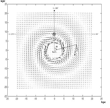
Figure 1: Direction and strength of the regular magnetic field in the Galactic plane is represented by the length and direction of the arrows. The field inside the Galactocentric circle of radius 4 kpc is taken as constant, 6.4 $\mu$G. The model was constructed using parameters from Stanev (1997) and Han et al. (1999), which are in detail described in the text. The sense and orientation of the field and of the angles $\Theta$ and $p$ follows from the figure. G.C. denotes the Galactic center (at $l=0^{\circ}$).

The global models omit the presence of turbulent fields and they are trying to model just the regular component. The basic conservative model of global Galactic plane was established by Han & Qiao (1994), based on the Faraday-rotation measurements of 134 pulsars. The model assumes a two-arm logarithmic spiral with the constant pitch angle $p$ and it shows $\pi$-symmetry, so that it is bisymmetric (BSS) magnetic field model. More exactly, it has also a dipole character (it has field reversals and odd parity with respect to the Galactic plane), so it is called BSS-A model.

Discussed model employs cylindrical coordinates — the radial distance $r$, the position angle $\Theta$ and the vertical height $z$. The radial $B_{r}$ and azimuthal $B_{\Theta}$ components at the plane position $(r,\Theta)$ can be given by the following equations:

$$B_{\Theta}=B_{0}(r)\cos\left(\Theta-\beta\ln\frac{r}{r_{0}}\right)\cos p,$$ (2)

$$B_{r}=B_{0}(r)\cos\left(\Theta-\beta\ln\frac{r}{r_{0}}\right)\sin p.$$ (3)

where $p$ denotes the pitch angle and according to Stanev (1997) and Han (2002) it is about $-10^{\circ}$, $\beta=1/\tan p\doteq-5.67$, $r_{0}$ is the Galactocentric distance of the maximum field strength at $l=0^{\circ}$ (in the discussed model it has a value $r_{0}=9.0$ kpc) and for $B_{0}(r)$ it holds:

$$B_{0}(r)=3\frac{R}{r},$$ (4)

where $R$ is the Galactocentric distance of the Sun, taken as 8.5 kpc.

The vertical ($z$) component of the field is taken as zero in approximate agreement with observations. Results of this model are depicted on Fig. 1 and the orientation of the whole system is also clear from this Figure.

The size and field strength in the Galactic halo is extremely important for the cosmic-ray trajectories, but it is very poorly known, as we stated above. Obvious approach to this problem is represented by the work of Stanev (1997), where the field above and under the Galactic plane is taken as exponentially decreasing:

$$|B(r,\Theta,z)|=|B(r,\Theta)|e^{(-|z|/z_{0})},$$ (5)

where $|B(r,\Theta)|$ is the vector sum of magnitudes of $B_{r}$ and $B_{\Theta}$ with the $z_{0}$ = 1 kpc.

We used this described model of GMF as the basis for our simulations. Strictly speaking, we simply add toroidal and poloidal field components to this model, as it is detailed in the next subsection.

Alternative models with another field configurations were also proposed. The another possible but according to recent observations a bit less probable configuration is the so-called ASS-S configuration, axisymmetric configuration without reversals and with even parity (Stanev (1997)). However, this configuration has one advantage. It could be much easier modeled using of the very popular dynamo model of magnetic field generation (Elstner et al. (1992)). The bisymmetric mode can also be obtained from dynamo model, but in such case the use of strong non-axisymmetric perturbations is necessary. The other two possibilities of magnetic field configurations — bisymmetric dipole type (BSS-S) and axisymmetric quadrupole type (ASS-A) are also not completely observationally excluded yet (Beck et al. (1996)).

2.3 Poloidal and toroidal regular field components

The dynamo model has one very interesting consequence for the propagation of CRs — namely that except of relatively flat field in the galactic disc it contains also quite strong toroidal fields above and under the galactic plane. Motions of these fields and their superpositions generate the net field in the Galaxy. The existence of such field is indirectly supported by the existence of radio thick disc mentioned above in the review of observation results. Such field could change the CR trajectories quite essentially, furthermore this type of models was not yet used for UHECR propagation simulation, therefore we decided to add these components in our simulations. We take advantage from the fact that only recently some first quantitative estimates of strengths of such fields were proposed by Han (2002).

For toroidal field we choose the model with simple geometry (circular discs above and under Galactic plane with Lorentzian profile in z-axis). For cartesian components of toroidal field it holds:

$$B_{x} = -B_{T}\sin(\phi)$$ (6)

$$B_{y} = B_{T}\cos(\phi)$$ (7)

For the value of $B_{T}$ we have:

$$B_{T} = B_{max}\frac{1}{1+(\frac{z-H}{P})^{2}}$$

for $$x^{2}+y^{2}<R^{2}$$ and

$$B_{T} = B_{max}\frac{1}{1+(\frac{z-H}{P})^{2}}\exp\left(-\frac{(x^{2}+y^{2})^{1/2}}{R}\right)$$

for $$x^{2}+y^{2}>R^{2}$$

where $x$ and $y$ are positions in Galactic plane. Meaning and values of used constants follow: radius of a circle with toroidal field $R=15$ kpc, height above Galactic plane $H=1.5$ kpc, half-width of Lorentzian distribution $P=0.3$ kpc, and maximal value of toroidal magnetic field $B_{max}=1\mu$G.

As consequence of existence of the poloidal field (dipole field) we probably observe vertical component of $0.2\mu$G in the Earth vicinity and intensive filaments near Galactic center. Appropriate equations, which we used for description of poloidal field, are the same as the equations for magnetic dipole. The field is symmetrical around Galactic axis. For the total poloidal field strength it is then valid (in xz-plane) in polar coordinates ($\theta$ ranges from 0 to $\pi$ and it goes from north to south pole):

$$B=\frac{K}{R^{3}}\sqrt{3\cos^{2}(\theta)+1}\mbox{.}$$ (10)

From it follows that in spherical coordinates we then have these cartesian field components:

$$B_{x} = -\frac{3K}{2R^{3}}\sin 2\theta\cos\phi$$ (11)

$$B_{y} = -\frac{3K}{2R^{3}}\sin 2\theta\sin\phi$$ (12)

$$B_{z} = -\frac{K}{R^{3}}(3\cos^{2}\theta-1)$$ (13)

A cylinder (height $300$ pc, diameter $100$ pc) with constant strength of magnetic field equal to $2$ mG was put into Galactic center instead of field resulting from equations above. Main motive for such arrangement was to avoid a problem with too strong field near this center ($R\sim 0$) and so to keep total field strength in observed bounds and to describe character of observed filaments.

The constant $K$ was selected as follows: $K=10^{5}$ G.pc³ for outer regions ($R>5$ kpc) and $K=200$ G.pc³ for central region ($R<2$ kpc). For the intermediate region (2 kpc $<R<$ 5 kpc) we used constant absolute field strength $10^{-6}$ G. These values correspond with observed features of Galactic magnetic field: milligauss field is restricted only to the central cylinder and the vertical magnetic field is equal to $0.2$ $\mu$G in the Sun’s distance (see also Fig. 2).

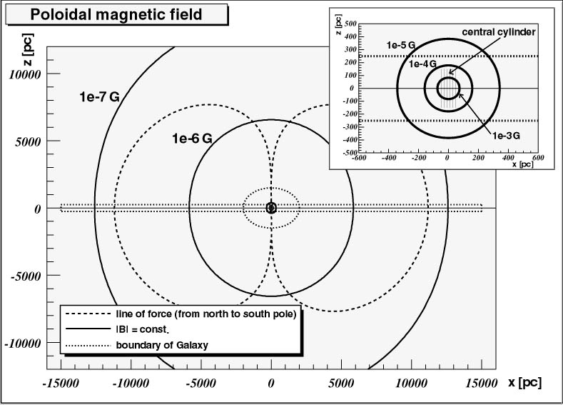
Figure 2: The resulting model of poloidal magnetic field. The central region is enlarged in the upper right corner.

2.4 Turbulent fields and Galactic arms

As we pointed out above, we introduce also the influence of random fields in our simulations. Cells with characteristic size of 50 pc with random field orientation and with maximum field strength $|B|=10\mu$G were added to regular, poloidal and toroidal field components.

Within two following examples we used two different approaches for introduction of turbulent fields. For study of chemical composition of CR (Example No. 2) various configurations (cell frequency, cell size) were used and are in detail described below. However, for directional analysis (Example No. 1) we respect the fact, that turbulent fields are common especially within spiral arms of Galaxy. Therefore we expect that 80% of volume inside spiral arm regions contain turbulent field component, while outside these arm regions only (but within surroundings of Galactic plane) 20% of total simulated volume have also nonzero turbulent field. Finally, in other outer regions of the Galaxy we suppose that only 1% of volume has also nonzero turbulent component.

As model of spiral arms we used model by Wainscoat et al. (1992), which is simple four-plus-local arm model. Parameters of this particular model are in detail described in Fig. 3.

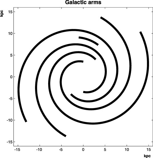
Figure 3: Model of Galactic arms by Wainscoat et al. (1992) has 4-arm pattern and it also includes so called Local arm. Equation for individual arms is: $\Theta(R)=\alpha\log(R/R_{min})+\Theta_{min}$, where $\alpha$ is winding constant, $R_{min}$ is inner radius and $\Theta_{min}$ angle at inner radius (Sun is positioned at y-axis.). Width of each arm is 750 pc, height 500 pc (centered on Galactic plane). Arms are truncated at distance 15 kpc from Galactic center. Parameters for individual arms follow in form (Arm No., $\alpha$ [rad], $R_{min}$ [kpc], $\Theta_{min}$, angular extent ($\Theta_{max}-\Theta_{min}$) [rad]): (1, 4.25, 3.48, 1.571, 6.0); (1’, 4.25, 3.48, 4.712, 6.0); (2, 4.89, 4.90, 4.096, 6.0); (2’, 4.89, 4.90, 0.953, 6.0); (Local, 4.57, 8.10, 1.158, 0.55).

3 Propagation of UHECRs in GMF

Within the next sections we describe two simple analyses of cosmic ray propagation in GMF. These analyses are done in different energy ranges and are serving for derivation of different conclusions, but they are involving the very same principles of particle motion in magnetic fields:

The propagation of the main part of UHECR (or more generally of cosmic rays) candidates (charged particles like protons, nuclei, electrons, …) is of course influenced by the magnetic fields. This influence is given simply by the well-known Lorentz equation. The member with electric field in this equation could be neglected, because there is no evidence for large-scale electric fields in the Galaxy. For the acceleration $\@vec{a}$ we get then:

$$\@vec{a}=\frac{q}{m}(\@vec{v}\times\@vec{B}),$$ (14)

where $q$ is the charge of particle, $m$ is its relativistic mass, $v$ its velocity and $B$ is the magnetic field strength.

Taking $\@vec{B}$ as constant in suitable small volumes the trajectory of a particle is followed and the resulting deflection is examined.

4 Application No.1: Directional analysis of UHECR

4.1 “Antiparticle tracing” method and recent works

Some computer simulations in the UHECR range were treated for this purposes recently and the effects especially on the changes in spatial distribution were studied.

The method of “antiparticle tracing” is used in all these models. The particle carrying the opposite charge starts its propagation on the position of the Earth in the Galaxy. Its initial velocity vector has spherical coordinates $\sim c,b,l$, where $c$ is the velocity of the light and $b$ and $l$ are the galactic coordinates of the detected particle arrival. Because of the opposite charge such particle traces backwards the trajectory of original detected particle. When the particle leaves from the sphere of influence of the Galactic magnetic field, we are able to evaluate its new galactic coordinates and thus its initial direction before the entrance into GMF.

The first work was published by Stanev (1997). It analyzes the motion of UHECRs in conservative models of BSS-A and ASS-S GMF with similar parameters as were given above. Stanev (1997) examines the shifts for protons with energies ranging from $(2\div 10)\times 10^{19}$ eV. The second article is by Medina Tanco et al. (1998). The particles with energy equal to $4\times 10^{19}$ eV are analyzed in this paper. The changes in regular distributions are followed for the ASS-S model of GMF and for the particles supposed to be either protons or Fe nuclei. The basic results of both models (magnitudes of deflections) are in good agreement with our model.

Two other papers appeared recently. In these papers the GMF model of Stanev (1997) was employed to support of specific arguments. Firstly, O’Neill et al. (2001) assumed iron nuclei as the only component of UHECRs and the authors were trying to identify the sources as very young pulsars. Secondly, Tinyakov & Tkachev (2001) investigated correlation between the positions of UHECRs propagated outside from Galaxy and of positions of specific type of blazars. They focused on possible identification of these blazars as UHECR sources and significant attention was payed also to analysis of clustered UHECR events.

Two other works propose the large Galactic magnetic halo with very intensive fields. The first article was published by Ahn et al. (1999), they speculate about large and intensive purely azimuthal magnetic field in the Galactic halo. This field should exist as an analogy to a solar wind and should extend to about 1.5 Mpc. In spherical coordinates $r,\theta,\phi$ it holds then

$$B_{\phi}=B_{S}R\frac{\sin\theta}{r},$$ (15)

where $B_{S}R$ is the normalization factor derived from the values in the solar surroundings, which is equal to 70 $\mu$G.kpc. If such field is introduced, the positions of 11 out of 13 EHECRs from Haverah Park, Volcano Ranch, Fly’s Eye and AGASA should fall within 20^∘ spherical cap around M87 position. This hypothesis was challenged shortly after its publication by Billoir & Letessier-Selvon (2000). They proved that this at the face-value exciting fact, that M87 could be a single source of UHECRs, is simply based on the fundamental property of the used magnetic field model in halo. The used model of an azimuthal field is simply focusing all positions into the direction of Galactic north pole and M87 is lying near to this pole, and so the small angular distance between computed EHECR positions and between M87 is probably just an interesting coincidence without fundamental physical importance. Furthermore, such strong magnetic halo is in contradiction with recent observations.

The second work was published by Harari et al. (2000) and it proposes the Galactic magnetic wind extending to 1.5 Mpc. The model examines focusing abilities of magnetic wind. Model of the magnetic wind used in this work is purely azimuthal:

$$B=B_{7}\frac{r_{0}}{r}\sin\theta\tanh\left(\frac{r}{r_{s}}\right),$$ (16)

It describes $B$ as a function of the radial spherical coordinate $r$ and the angle to the north galactic pole $\theta$. The term $r_{0}$ in this equation is the distance from the Earth to the Galactic center (equal to 8.5 kpc), factor $r/r_{s}$ was introduced to smooth out the field at small radii ($r_{s}$ was taken as 5 kpc). $B_{7}$ is the normalization factor (the strength of the field in [7 $\mu$G] units) and so in conservative models of GMF $B_{7}$ should be $\sim 0.3\div 0.4$. As it is shown in our combined Fig. 4, such magnetic field has to sweep out some fraction of the southern Galactic hemisphere. However, using the data from SUGAR which are also plotted into this figure, we are able to show that such a model could not be completely correct. This is due to the fact that these regions with proposed zero particle flux — in contrary to the theoretical expectations — contain several SUGAR events.

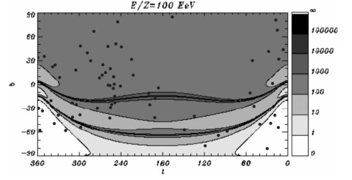
Figure 4: Contour plots of the amplification of cosmic-ray flux by the Galactic wind (according to Harari et al. (2000)). The plotted dependance of the flux on arrival directions to the Earth was computed for initial isotropic distribution of point sources (outside of the Galaxy) and for $\bar{E}=10^{20}$ eV. Figure was superposed with coordinates of SUGAR events (black dots) of the arrivals of most energetic particles ($\geq 4\times 10^{19}$ eV according to Hillas E model of energy estimation of SUGAR events). There are some SUGAR events inside of the white triangle-shaped areas (bottom corners), where the zero cosmic-ray flux is expected.

Finally, two interesting works treating the turbulent fields appeared recently. Alvarez-Muñiz et al. (2002) carefully analyzed the influence of turbulent fields on possible clustering of UHECRs and Harari et al. (2002) made large study of properties of typical turbulent fields with respect to amplification and multiplication of source images.

4.2 Computer Model

In our simulation we have supposed the conservative Galactic magnetic field model by Han et al. (1999), which was amended with toroidal and poloidal field components and with turbulent fields linked to spiral arms; this complete configuration of magnetic field was discussed in detail above.

Despite using various types of initial data, we present here only the results for real data. Namely, even such constrained set of data can sufficiently demonstrate all important changes of features of particle flux. These real data were taken from our catalogue of UHECRs. We propagate these particles through Galactic magnetic field assuming various charges — starting as protons (proton number $Z=1$), continuing as oxygen nuclei ($Z=8$) and ending with iron nuclei ($Z=26$). All particles were traced back off the influence of Galactic field. The final distance of each particle was assumed to be 40 kpc from Earth. We present here (Figure 5) the results of simulations corresponding the real UHECR data (145 UHECR positions and energies) taken successively as protons, oxygen and iron nuclei.

Figure 5: The original arrival directions (in galactic coordinates) of 145 UHECRs are shown in the uppermost part of the Figure. The other three sky-maps (all in galactic coordinates) are showing the final positions of cosmic ray particles which were propagated to the distance 40 kpc from the Earth. The second map from the top shows final positions of protons (the average angle between the initial and final position of individual particle is $2.9^{\circ}\pm 1.6^{\circ}$ [s.e.]). The third map shows final positions of oxygen nuclei (average angle $23^{\circ}\pm 12^{\circ}$ [s.e.]) and finally the fourth map shows positions of iron nuclei (average angle $72^{\circ}\pm 38^{\circ}$ [s.e.]).

4.3 Results of particle tracking

We can state that the given deflection ranges (Fig. 5) are in good agreement with previous models (Stanev (1997), Medina Tanco et al. (1998) or O’Neill et al. (2001)) of propagation of UHECRs through the Galactic magnetic field. Hence we can formulate the following conclusions:

• As we already stressed above, the detail of global structure of GMF is still uncertain, but despite that we can claim that its influence is non-negligible for protons and essential for Fe nuclei.

• The simulations of particles with higher charges (e.g. oxygen or iron nuclei) are transforming the isotropic distribution to structures, which show some regularities. The actual forms of these regular structures are as well as the global model of GMF rather uncertain, but their existence could be taken for granted and it is independent on the specific parameters of given magnetic field model. In accordance with Harari et al. (2002) we observe especially for oxygen and iron nuclei (Fig. 5) that at some places the initial flux is amplified, in other areas it is strongly suppressed (see e.g. overdensity in region to north-west from Galactic center for both oxygen and iron nuclei or almost empty region along Galactic plane again for both type of nuclei).

• GMF is very important also for protons, because it is able to affect the small-angle clustering (as one can see on the second upper part of Fig. 5, where some initial small clusters were transformed into other ones). Small-angle clustering is today lively discussed and it is one of the key features in discrimination between some models of sources (Alvarez-Muñiz et al. (2002)).

• The possibility that the UHECRs originate in the Galaxy (e.g. near the young neutron stars in the form of iron nuclei) is not probable, but not completely excluded (see the bottom part of Fig. 5). Furthermore, such UHECRs should originate only in several point sources in our Galaxy, what is again in accordance with the existence of pseudo-regular structures after propagation through the GMF (see also O’Neill et al. (2001) or Harari et al. (2002)).

The theory of Galactic origin of UHECRs could be also combined with the above discussed fact that also relatively strong ($\sim 1$ mG) fields exist in the form of filaments near Galactic center. In such field the Larmor radius of $10^{19}$ eV UHECR proton is only about 4 pc.

5 Application No.2: Chemical composition of CRs

5.1 Propagation of CRs in our model

We used very simple method to model the propagation of cosmic ray particles in a rather wide range of energy ($10^{13}\div 10^{19}$ eV). The model of regular magnetic field described above was improved with following configuration of turbulent components:

The Galaxy was divided into cubic cells of an assumed size $L$. Two values of cell length were studied, in particular 10 and 50 pc. The random orientation and strength of the turbulent magnetic field were generated in given fraction of cells and also their positions were random. In accordance with observation the contribution of the turbulent magnetic field was taken equal to $(0\div 3)\times B(r,\theta,z)$, where $B(r,\theta,z)$ is sum of strengths of the non-turbulent components. We neglected all possible interactions of particles with matter and we kept the energy of particles constant.

Our Galaxy model has the following geometrical boundary: the bulge is a symmetric ellipsoid with a major axis in the Galactic midplane 3 kpc long and a minor axis of 2 kpc. Around the bulge there is a thin cylinder with a radius of 15 kpc and the height of 500 pc. Starting positions of particles reside in the Galactic plane inside an annulus with radii of 3 and 12 kpc. This assumption is in the agreement with the observed positions of supernovae remnants (Green (2001)), which are the most probable sources of CRs below the knee in our Galaxy.

As Gaisser (2001) and Brunetti & Codino (2000) have shown, the average time spent in the Galaxy by cosmic ray of energy within the range $(1\div 100)\times 10^{9}$ eV is $\tau\sim 10^{14}$ s. The energy dependence of $\tau$ can be measured by comparing the spectrum of the secondary nuclei to that of the parent primary nuclei. From observation one can deduce that at least in the range $10^{10}\div 10^{12}$ eV, the mean residence time varies approximately as $R^{-0.6}$ (Garcia-Munoz et al. (1987), Swordy et al. (1990) and Engelmann et al. (1990)), where $R=\frac{pc}{Ze}$ is the rigidity of particle with momentum $p$ and atomic number $Z$. This extrapolation breaks down around $3\times 10^{15}$ eV (Gaisser (2001)) because the value of an effective escape length is equal to $c\tau\sim 300$ pc which corresponds to just one crossing of the Galactic disk and the probability of nuclei escape significantly rises. The situation within the highest energy range is not clear, but we expect that the nuclei are not trapped in GMF. The task we have to solve is to find the value of tracking time for the simulation of particles with energies in range $10^{13}\div 10^{19}$ eV. We have found that the value $T=3\times 10^{12}$ s $\sim 10^{5}$ yr appears as the most suitable tracking time of particles for the study of nuclei escape rate from the Galaxy. From the equation $\tau\sim R^{-0.6}$ we obtain the value $10^{11}$ s for proton with the energy in the middle of our range (which is equal to $10^{15}$ eV). Despite of it, we use tracking time longer by one order of magnitude. The reason for such choice is that: (1) The mean residence time for nuclei with higher $Z$ will be longer than for proton. (2) The nuclei escape rates are too high (too low) for longer (shorter) tracking times and as such they are not suitable for discrimination between the different nuclei. (We note that we use only one value of tracking time for whole energy range of particles.)

The propagation of particle was stopped in a moment when the particle escaped from the Galaxy. The escape occurred when the particle crossed the Galaxy geometrical boundary. Otherwise, if the particle stayed within the Galaxy for time longer than $T=3\times 10^{12}$, simulation was also stopped and the particle was simply taken as not escaped. From these values of the particle escape rates one can easily calculate the chemical composition of CRs.

Our starting chemical composition is taken from Wiebel-Sooth et al. (1998), who summarized results of several experiments for energy $10^{12}$ eV. We have divided all nuclei into five groups according to their mass. From each group we choose a nucleus that is the best representative. In this way we have chosen protons and nuclei of helium, oxygen, magnesium and iron as group representatives, with initial abundance equal to $42\%$, $26\%$, $13\%$, $9\%$ and $10\%$, respectively. As the indicator of the composition, we use mean value of the logarithm of mass number $A$,

$$<\ln(A)>=\frac{\sum n_{i}(\ln(A_{i}))}{\sum n_{i}},$$ (17)

where $n_{i}$ denotes the number of elements $i$ with mass number $A_{i}$. The initial composition at $10^{12}$ eV is $<\ln(A)>=1.41$ (Wiebel-Sooth et al. (1998)).

Figure 6: An example of nuclei escape rate from GMF improved by turbulent MFs located in 40 percents of cubic cells with size equal to 10 pc.

5.2 Results and conclusions

We have used only one above discussed model of GMF in our simulation, although it was improved by random components of the turbulent magnetic field. We have confirmed the influence of such turbulent magnetic fields on the propagation of CRs for all studied nuclei energies.

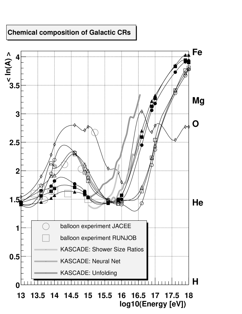
Figure 7: Change of nuclei composition as a result of nuclei escapes from Galactic disk compared with experimental results. The line with diamonds correspond to modelling without turbulent magnetic field, the lines with circles, squares and triangles indicate number of cells with turbulent magnetic field equal to 10 %, 20 % and 40 % respectively; filled for dimension of cells equal to 50 pc and empty for 10 pc.

We find following results in our simulation:

• The dependence of nuclei escape rate on the energy is similar for all configurations of magnetic fields (Fig. 6). Except configuration without turbulent magnetic field all values of nuclei escape rate are lower than 7% at our starting energy $10^{13}$ eV (even for protons). Thereafter up to $10^{15}$ eV the leakage depends on the charge, the higher charge, the lower is number of nuclei escape rate. In the energy range $10^{15}\div 10^{16}$ eV the nuclei escape rate of light nuclei (H, He) becomes constant and the values of heavier elements come closer to them. The differences between cells with dimension equal to 10 pc are 10%, the lowest value is for the configuration with the highest rate of the cells with turbulent magnetic field. The situation for the cell dimensions equal to 50 pc is similar but the values are much closer and lies around $(78\pm 2)$%. Nuclei with energies higher than $10^{16}$ eV behave in the same way as at the energy below $10^{15}$ eV. It is again a function of particle charge and we can observe an increase of the abundance of heavy elements (Fig. 7). Escape rate achieves 100% for protons (all protons leave the Galaxy) at energy equal to $4\times 10^{17}$ eV. Protons are closely followed by nuclei of helium and for energies higher than $10^{18}$ eV no particle will remain in Galactic disk.

• We have found that more than 90% of the particles above $10^{16}$ eV are escaping independently of their charge from the regular magnetic field. We believe that the different nuclei escape rate for the energies above $10^{16}$ eV is caused mainly by random component of GMF.

• The leakage of nuclei from the Galaxy depends significantly on the characteristics of turbulent magnetic fields (field’s strength, their dimensions and locations in the Galaxy and also on the number of cells with turbulent magnetic field). It follows from our simulations that the higher the fraction of the cells with turbulent magnetic fields, the slower is the leakage. This is because of the nuclei are trapped in these cells and their leakage from the Galaxy decreases. Unfortunately all properties of turbulent magnetic fields, which are very important for the propagation of CRs, are not known enough.

• The behavior of protons and helium nuclei is very similar in the whole studied energy range. They escape more easily than nuclei with higher charge (oxygen, magnesium and iron). Despite of this, they still play important role in CRs, because of their dominant abundance in the initial composition of CRs (representing together more than two thirds of all particles).

• The result of the different nuclei escape rate is the increase of the abundance of heavier nuclei in the chemical composition of CRs. The comparison of the chemical composition resulting from our modelling with the measurements is shown in Fig. 7. Experimental data show unique results only for the energies below $10^{14}$ eV, where they show slight increase of mean $\ln(A)$. Above $10^{14}$ eV the results of two balloon experiments JACEE (Takahashi (1998)) and RUNJOB (Apanasenko et al. (2001)) disagree. RUNJOB shows no change in the chemical composition (constant value of mean $\ln(A)$), whereas data from JACEE indicate increase of mean $\ln(A)$. The experimental results from RUNJOB are in agreement with our results — for our model with turbulent magnetic fields with cell dimensions equal to 10 pc. In the case with larger dimension of cells (50 pc) we have found higher leakage of light nuclei (proton and helium) which leads to the same increase of mean $\ln(A)$ as measured by JACEE.

  For energies above $10^{15}$ eV we have chosen only data from KASCADE (Haungs (2002) and Hörandel (2002)). Two methods of data processing show increasing mean $\ln(A)$ from the value equal to the initial composition at $10^{12}$ eV to the value, when the majority of cosmic rays is composed of heavy elements. Third method (neural net) gives different results, firstly decrease from the value $<\ln(A)>=2$ to the initial value and above energy equal to $10^{16}$ eV increase to high value of mean ln(A).

  The results of our modelling have following characteristics above $10^{15}$ eV: The modelling with only regular GMF does not agree with experimental data, while the cases with turbulent MF show correctly the increase of the abundance of heavy elements at high energies. The discrepancy between our model with turbulent MF and measurements is in the value of the energy, where the increase of mean $\ln(A)$ starts. If we take the energy equal to $3\times 10^{15}$ eV (knee) as correct, then the differences will be half magnitude and one magnitude for dimensions of cells equal to 10 and 50 pc, respectively. We have found that this discrepancy does not strongly depend on general parameters of our modelling (the tracking time and thickness of Galactic disk), we believe that this discrepancy can be removed only using more realistic method of modelling motion of atomic nuclei (for review see Gaisser (1990)).

• The different leakage of nuclei from GMF produces a break at energy $10^{16}$ eV in our modelling, similar to observed characteristic of cosmic ray flux, known as the knee ($3\times 10^{15}$ eV). Thus our simple model of the propagation of Galactic cosmic rays favors theory about origin of the knee presented by Ptuskin et al. (1993).

• The model of propagation in GMF without turbulent MF seems to us as very unrealistic, because there is in strong disagreement with measurements.

• We can see that the chemical composition depends on the characteristics of turbulent MF, so it gives us possibility to deduce these characteristics from the abundance of elements in Galactic cosmic rays.

The used method is a simple way to simulate the propagation of CR within wide energy range. Despite of good obtained results we conclude that the propagation of particles must be solved by more realistic method, especially for particles with energies below $10^{16}$ eV. We used only one type of the source in the Galactic midplane with constant chemical composition. However, there are indications that we must expect more types of sources in the Galactic and extragalactic space resulting in more complicated cosmic ray flux.