Interstellar Hydroxyl Masers in the Galaxy. II. Zeeman Pairs and the Galactic Magnetic Field

Abstract

We have identified and classified Zeeman pairs in the survey by Argon, Reid, & Menten of massive star-forming regions with 18 cm (${}^{2}\Pi_{3/2},J=3/2$) OH maser emission. We have found a total of more than 100 Zeeman pairs in more than 50 massive star-forming regions. The magnetic field deduced from the Zeeman splitting has allowed us to assign an overall line-of-sight magnetic field direction to many of the massive star-forming regions. Combining these data with other data sets obtained from OH Zeeman splitting, we have looked for correlations of magnetic field directions between star-forming regions scattered throughout the Galaxy. Our data do not support a uniform, Galactic-scale field direction, nor do we find any strong evidence of magnetic field correlations within spiral arms. However, our data suggest that in the Solar neighborhood the magnetic field outside the Solar circle is oriented clockwise as viewed from the North Galactic Pole, while inside the Solar circle it is oriented counterclockwise. This pattern, including the magnetic field reversal near the Sun, is in agreement with results obtained from pulsar rotation measures.

1 Introduction

Hydroxyl (OH) masers are an excellent tool for probing the environment of massive star-forming regions (SFRs). They are bright and easily observable and act as point tracers of the local velocity and magnetic fields, owing to their large Zeeman splitting coefficient. For the ground-state ${}^{2}\Pi_{3/2},J=3/2$ transitions, the Zeeman splitting coefficient is as large as 0.59 km s^-1 mG^-1. For a typical maser linewidth of 0.3 km s^-1, a milligauss-strength magnetic field is sufficient to cleanly separate Zeeman components of the 1665 MHz transition, and even fields as weak as several hundred microgauss can be detected. In addition, the sense of the splitting indicates the projected line-of-sight magnetic field orientation.

Davies (1974) first hypothesized that a connection exists between magnetic field directions obtained from molecular Zeeman splitting and a large-scale Galactic magnetic field. He found that eight OH maser sources (and several H I clouds) mostly near the Solar circle with observable Zeeman splitting displayed magnetic fields aligned in the clockwise direction when viewed from the North Galactic Pole. Reid & Silverstein (1990) conducted a literature search and found a total of 17 reliable OH maser sources with detectable Zeeman pairs in the ${}^{2}\Pi_{3/2},J=3/2$ transitions. Of these 17, 14 had line-of-sight field directions consistent with an overall clockwise Galactic field. In the largest survey to date, Baudry et al. (1997) extended this dataset to include a total of 46 sources with Zeeman pairs in the ${}^{2}\Pi_{3/2},J=3/2$ and $J=5/2$ transitions of OH. Excluding the Galactic center, they found 28 sources consistent with a clockwise magnetic field and 17 sources consistent with a counterclockwise field.

Argon, Reid, & Menten (2000, henceforth Paper I) conducted a survey of 91 interstellar regions with known ${}^{2}\Pi_{3/2},J=3/2$ OH maser emission. They identified and mapped maser spots in the regions. In this paper we extend the analysis of Paper I by identifying Zeeman pairs toward massive SFRs, many of which contain ultracompact (UC) H II regions. We also investigate whether or not the magnetic fields deduced from OH Zeeman splitting around massive SFRs are related to the large-scale magnetic field of the Galaxy.

2 Observations

A total of 91 maser sources were observed by Paper I with the A configuration of the National Radio Astronomy Observatory’s Very Large Array in Socorro, NM. All sources were observed in both left- and right-circular polarization in at least one main-line ${}^{2}\Pi_{3/2},J=3/2$ 18 cm OH transition (1665.4018 and 1667.3590 MHz), and some were also observed in one or both of the satellite-line transitions (1612.2310 and 1720.5300 MHz). The 0.763 kHz spectral channel separation used corresponds to a velocity separation of 0.14 km s^-1 for the main-line transitions (FWHM $\sim 20\%$ larger). Further details of the observations can be found in Paper I.

3 Zeeman Pair Selection Criteria

In the presence of a magnetic field, the degeneracy of the magnetic sublevels of the OH molecule is broken. For any given hyperfine transition, this results in three or more spectral lines with differing polarization properties — the Zeeman effect (see Davies, 1974, for more details). OH masers often display pairs of strong left and right elliptically polarized $\sigma$-components. For reasons that are not well understood, purely linearly polarized $\pi$-components are rarely, if ever, detected.

The task of identifiying Zeeman pairs — two oppositely elliptically polarized lines at the same position on the sky — is relatively simple, provided one has sufficient angular resolution to resolve maser clusters (e.g., Reid et al., 1980). However, with the VLA one can only achieve an angular resolution of $\approx 1$ arcsec for the OH transitions at wavelengths of 18 cm. Were the emission in any spectral channel to come from only one (unresolved) spot on the sky, this would not be a significant limitation. However, in reality the emission in any given spectral channel can come from spectral blends of masers at different positions in the source separated by less than the beam size. Thus, great care must be taken to determine Zeeman pairs from the Paper I data.

In order to identify Zeeman pairs, a modified version of the NRAO Astronomical Image Processing System (AIPS) task JMFIT was used to identify the brightest maser emission spot in each spectral channel (velocity plane) for any given source. A maser line was identified when emission was seen from approximately the same position in at least three adjacent velocity channels, with the strongest emission not found on the edge channels. This resulted in a large data set that could be automatically searched for Zeeman pairs.

Ideally, one would like to find Zeeman pairs in which the oppositely circularly polarized components were coincident on the sky to better than their apparent spot sizes. However, Reid et al. (1980) showed that OH masers in W3(OH) clustered on a scale of $3\times 10^{15}$ cm ($0\arcsec\!\!.09$ at 2.2 kpc; distances are discussed in §4.1 and listed in Table 1) and that oppositely circularly polarized maser lines within a cluster gave reliable magnetic field measurements when interpreted as Zeeman pairs. Thus, we searched for oppositely circularly polarized maser lines with projected positions separated by less than $3\times 10^{15}$ cm. While the main-line 1.6 GHz $\sigma$-components are in general elliptically polarized, it is almost functionally equivalent to treat them as being circularly polarized for the purposes of right-circular polarization (RCP) and left-circular polarization (LCP) VLA data. The caveat is that, for example, a right-elliptically polarized maser component, being the sum of circularly and linearly polarized emission, may appear in both RCP and LCP data at the same velocity, although the LCP emission will be much weaker, as the LCP feed is sensitive to only half of the (presumed small) linear component of the full elliptical polarization.

Some Zeeman pairs consisted of single RCP and LCP lines that were coincident on the sky to better than $3\times 10^{15}$ cm. We consider these easily recognizable and reliable Zeeman pairs. However, more than one maser line in the same polarization would often be seen within the assumed $3\times 10^{15}$ cm clustering length, such that it was unclear which should be paired with the maser spot in the other polarization. While such data are insufficient to make an unambiguous Zeeman pair identification in all such cases, sometimes corroborating evidence from another maser transition (or occasionally even the same transition) in the same spatial region allowed the identification of Zeeman pairs. In other cases, the line-of-sight field direction was deducible, even if unambiguous identification of a Zeeman pair was not possible, for example, when multiple LCP and RCP lines were seen, but each RCP line was at a higher velocity than any of the LCP lines. We felt it important to generate specific, objective, criteria that allowed an algorithmic approach to search for Zeeman pairs and accept or reject them without resorting to a visual examination of spectra on a case-by-case basis, which can lead to significant unquantifiable biases. Below we describe how we handled each of the complications.

For any given source, a “window” of radius $3\times 10^{15}$ cm was centered on the strongest line in either polarization in a single transition. In principle, if the window included one line in each polarization, the lines would be identified as a Zeeman pair. However, emission channels key to identifying the second maser line in a Zeeman pair sometimes lay just outside the window when it was centered on the position of brightest emission, whereas were the window moved between the position of the lines, it would pass the $<3\times 10^{15}$ cm separation criterion. To overcome this problem, the window center was moved from the centroid of strongest emission along a grid, in increments of 5% of the window radius, out to a maximum displacement of 50% of the radius in both the R.A. and Dec directions. The window containing the largest number of lines was used, provided that at least one line of each polarization was included. “Tiebreaker” criteria consisted first of choosing the window with the largest number of velocity channels represented and second of choosing the window whose offset from the grid center was smallest. Next, all velocity channels contained in the chosen window were flagged as used, and the process was iterated with the remaining maser spots. In this way, the entire source was partitioned into windows consisting of potential Zeeman pairs. This partitioning was done independently for each maser transition for which data were collected for the source.

Identification of Zeeman pairs in windows containing only one maser line in each polarization is straightforward. Figure 1a shows spectra from two windows for G351.775$-$0.538, one in each of the 1665 and 1667 MHz transitions. The 1665 MHz window contains two oppositely circularly-polarized maser lines. Removing the effects of the Zeeman splitting from a magnetic field of $-3.80\pm 0.03$ mG (i.e., oriented in the hemisphere toward the Sun.), the center velocity of the emission would be at $-26.74\pm 0.02$ km s^-1. The 1667 MHz window, centered 120 mas away, shows a similar splitting of $-3.66\pm 0.06$ mG centered at a velocity of $-26.79\pm 0.02$ km s^-1. While a large fraction of the Zeeman pairs we identified were found in windows containing exactly one maser line in each polarization, a few of these pairs appeared with a corroborating nearby pair of a similar magnetic field in another transition.

Table 1 is a list of Zeeman pairs with “non-zero” velocity separation. The flux, velocity, and velocity width of lines was determined by a Gaussian fit to the center 5 channels of each line when available, else to 4 or only 3 channels. (By our criteria for a maser line, the center 3 channels must necessarily be detected.) Pairs are only included in this table if the velocity difference between the LCP and RCP lines exceeds twice the signal-to-noise-limited velocity error, taken to be the sum in quadrature of the HWHM line width divided by the signal-to-noise ratio of each of the lines. However, in no case is a pair of lines allowed to satisfy this criterion if the velocity center separation is less than 5% of the quadrature sum of the line widths, or typically about 0.02 km s^-1. These “pairs” may be actual Zeeman pairs with a small splitting due to a small magnetic field, or they may be single maser spots with a large linear polarization fraction, but the limited spatial and velocity resolution of the VLA and the absence of full-polarization observations render it difficult to decide between these two cases. These “near zero” velocity separation maser spots are listed in Table 2.

While identification of many of the pairs listed in Table 1 was straightforward, not all windows were so simple to interpret. When a window contains more than one maser line in a polarization, interpreting the Zeeman pattern is more complicated. In this case, it may still be possible to know the light-of-sight direction of the magnetic field, but not its strength. Figure 1b shows the spectrum of one window associated with G032.744$-$0.076. There is one RCP maser line (labelled 1) centered at 32.38 km s^-1 and two LCP lines (2 and 3) at higher velocities (34.60 and 35.02 km s^-1, respectively). Additionally, there is one feature (4) that does not meet our criteria as a maser line, since the low-velocity side of the line is not seen, probably owing to blending with a stronger line elsewhere in the source. It is unclear which LCP line should be associated with the RCP line as a Zeeman pair. Regardless of the exact pairing, the RCP line is at lower velocity than any LCP line, so the line-of-sight orientation of the magnetic field is known to be pointed toward the Sun. Cases such as this, where the field direction is known but its strength is not, are frequent among our data. When a range of values is quoted for the magnetic field in Table 1, the direction of the magnetic field is well-determined, and the smallest and largest possible magnetic field intensities are given. Some line parameters not listed in the table are given in the notes on individual sources.

Sometimes when a window contains enough maser lines such that the magnetic field strength or direction is ambiguous, supporting evidence may exist to suggest one pairing above all others. If a pairing in one transition implies a magnetic field strength and direction consistent with that of a pair in another transition at nearly the same location, that pairing is accepted in preference to all other possible pairings. Figure 1c shows a 1665 MHz and a 1667 MHz window in K3$-$50, coincident to within 46 mas. In each window, there is one RCP line (1) at lower velocity than either of the two LCP lines (2 and 3), so the line-of-sight field is oriented toward the Sun. But the field magnitude can also be deduced, assuming that the nearly overlapping windows in the two transitions are measuring the field at approximately the same location. In the 1665 MHz window, pairing lines 1 and 2 would give a magnetic field of $-1.5$ mG, while the 1–3 pairing implies a $-2.5$ mG field. In the 1667 MHz window, the 1–2 pairing yields $-0.8$ mG, while 1–3 yields $-2.6$ mG. The close agreement between the field values for the 1–3 pairs for the two transitions suggests that these Zeeman pairs should be favored over the other pairing possibilities. For definiteness, when appealing to corroborating evidence from one transition to resolve pairing ambiguities in another transition, we required $\Delta B\leq 0.4$ mG, $\Delta v_{c}\leq 0.2$ km s^-1, and $\Delta\theta\leq 0\arcsec\!\!.2\sec z\tan z$, where $\Delta B$ is the difference of the implied magnetic field strengths, $\Delta v_{c}$ is the separation of the center velocity of each pair, $\Delta\theta$ is the positional offset between pairs, and $z$ is the zenith angle of the source as viewed from the location of the VLA at transit. As noted in Paper I, relative positional offsets between different OH transition frequencies are $\approx 0\arcsec\!\!.1$ for high-declination sources, but grow to several arcseconds for sources at very low declination ($\lesssim-40\arcdeg$). The function “$\sec z\tan z$” was chosen in the spirit of the plane-parallel approximation for the atmospheric contribution to the relative error between observations of different transitions (see Reid et al., 1999).

If two pairings in the same window in the same transition imply the same magnetic field direction and strength, those pairings are also accepted over all other pairings. This situation arises when two Zeeman pairs in the same transition are encompassed in the same window. Figure 1d shows a 1665 MHz window for G45.465$+$0.047 that contains a cluster of maser lines. Since all of the RCP lines are at a higher velocity than the LCP lines, the magnetic field is oriented away from the Sun. However, the velocities associated with the line centers favor two particular pairings: pairing lines 1 and 4 yields a magnetic field strength of 3.7 mG, and 2 and 5 yield 3.8 mG.

Occasionally, a window would produce a spectrum with a clear, strong line in one polarization and an incomplete line in the opposite polarization. A closer look at the data would show that one or two critical points of the incomplete line lay just outside the window. By increasing the size of the window, a Zeeman pair was often identified. Using a larger window (generally twice the clustering radius) can be justified for two reasons. First, the window radius of $3\times 10^{15}$ cm is based on the clustering scale analysis of Reid et al. (1980), which is itself based on only one source: W3(OH), assuming the photometric distance of 2.2 kpc (Humphreys, 1978). The kinematic distance of 4.3 kpc, assuming the NH₃ LSR velocity of $-45$ km s^-1 (Reid, Myers, & Bieging, 1987) and a flat $R_{0}=8.5$ kpc, $\Theta(R)=220$ km s^-1 rotation curve, would correspond to a clustering scale of $6\times 10^{15}$ cm, or twice that which is derived from the photometric distance. In any case, it is unclear to what extent this varies among massive SFRs. Second, the distance to some of the massive SFRs is unknown. If the assumed distance to the source is greater than the actual distance, the (angular) window radius used would be proportionally smaller than the desired $3\times 10^{15}$ cm. For sources for which the kinematic distance ambiguity has not been resolved, the Zeeman pair identification analysis was done twice, assuming each of the near and far distances for calculation of the clustering scale. Zeeman pairs identified assuming either distance were accepted and are listed in Table 1. Despite the distance uncertainty, we believe that Zeeman pairs identified around these sources are still reliable indicators of the local magnetic field. When the far kinematic distance is more than a few times the near kinematic distance, possible errors involve partitioning a far source into windows that are too large or a near source into windows that are too small. In the former case, nearly all of the maser emission of a source (presumedly) located at the far kinematic distance would be concentrated in a single window when the near distance was used for the angular clustering scale, resulting in confusion of Zeeman pairs. In the latter case, a (presumed) near source would be micropartitioned into windows of small radius, rejecting many Zeeman pairs coincident to within the desired linear clustering scale. Thus, misresolving the near/far kinematic distance ambiguity results in the identification of fewer Zeeman pairs, regardless of whether a far source is assumed to be near or a near source is assumed to be far.

Zeeman pairs were also graded to reflect the uncertainty in pairing. Pairs from windows containing only one line in each polarization were assigned a grade of B, unless they were confirmed by a similar pair in a second transition, in which case they were given a grade of A. All pairs whose pairing was ambiguous were given a grade of C, even if the ambiguity was resolved by appealing to a second pair in the same or another transition. Pairs for which the separation of the Zeeman components exceeded the default window size were assessed a grade of D. In one case in G081.871+0.781, a grade of D was assigned to a Zeeman pair believed to be spurious; for further details see §4.3. This grading system is in the spirit of, although not identical to, the system used in Reid & Silverstein (1990), in which the main emphasis was on whether interferometry was used to identify Zeeman splitting, and if so, at what resolution. All of the Zeeman pairs listed in Table 1 were identified using interferometry.

Table 1: Zeeman Pairs

				LCP			RCP
		Dist.	Freq.	$S$	$v_{\mathrm{LSR}}$	$\Delta v$	$S$	$v_{\mathrm{LSR}}$	$\Delta v$	$\Delta\theta$	$B$
Source	Alias	(kpc)	(MHz)	(Jy)	(km s-1)	(km s-1)	(Jy)	(km s-1)	(km s-1)	(arcsec)	(mG)		Grade
G000.547$-$0.852	RCW 142	7.3	1667	0.23	8.96	0.65	3.72	6.33	0.43	0.046	–7	.4	B
G000.666$-$0.034	Sgr B2M	8.2	1720	6.84	61.09	0.28	14.21	61.25	0.32	0.028	0	.7	B
G000.670$-$0.058	Sgr B2	8.2	1612	3.78	67.40	0.87	3.91	67.24	0.82	0.024	–0	.7	D
G005.886$-$0.393	$\cdots$	3.8	1665	4.26	9.52	0.26	3.04	10.41	0.32	0.028	1	.5	A
			1667	8.90	9.71	0.28	7.83	10.22	0.29	0.012	1	.4	A
				1.43	4.93	0.75	0.74	5.18	0.96	0.042	0	.7	B
				1.07	6.10	0.80	1.50	7.08	0.56	0.080	0.2	$\rightarrow$2.8	C
G009.622$+$0.195	$\cdots$	5.7	1665	2.41	–1.07	0.42	8.06	1.75	0.37	0.018	3.9	$\rightarrow$9.7	C
				1.34	3.90	0.53	2.68	3.85	0.40	0.044	–0.1	$\rightarrow$–5.4	C
			1667	9.67	1.47	0.41	1.98	1.43	0.48	0.043	–0	.1	B
G010.624$-$0.385	$\cdots$	4.8	1667	43.03	–0.59	0.35	44.13	–1.98	0.25	0.045	–3	.9	B
				0.80	2.08	0.30	1.26	0.10	0.33	0.049	–5	.6	B
G012.216$-$0.117	$\cdots$	3.3	1665	15.26	29.07	0.49	12.32	27.55	0.50	0.042	–2	.6	B
G012.680$-$0.181	W33 B	4.0	1665	20.29	64.45	0.50	4.45	63.34	0.43	0.035	–1.9	$\rightarrow$–6.3	C
			1667	5.45	64.50	0.48	3.62	62.50	0.62	0.029	–0.7	$\rightarrow$–7.5	C
G012.908$-$0.259	W33 A	4.0	1667	69.34	39.93	0.49	5.12	40.41	0.75	0.023	1	.4	B
G017.639$+$0.155	$\cdots$	2.1	1665	1.79	20.92	0.35	2.22	20.42	0.28	0.048	–0	.8	B
G020.081$-$0.135	$\cdots$	12.3	1665	0.66	42.90	0.48	2.22	48.64	0.39	0.060	9	.7	B
				10.99	46.60	0.39	1.42	49.75	0.48	0.016	5.3	$\rightarrow$7.3	C
G028.199$-$0.048	$\cdots$	5.7	1665	11.48	94.92	0.36	19.23	94.89	0.27	0.008	–0	.1	B
G031.412$+$0.307	$\cdots$	6.2	1667	3.50	103.84	0.57	2.80	103.48	0.60	0.013	–1	.0	B
G032.744$-$0.076	$\cdots$	2.3	1665	0.61	32.84	0.67	0.68	31.00	0.56	0.099	–3	.1	B
				1.04	35.02	0.58	1.73	32.38	0.46	0.059	–3.8	$\rightarrow$–4.5	C
				0.39	36.44	0.37	0.92	39.58	0.35	0.053	5.3	$\rightarrow$6.4	C
G034.257$+$0.154	$\cdots$	3.8	1665	16.04	58.14	0.37	79.02	58.22	0.38	0.015	0	.1	B
			1667	108.48	58.64	0.38	66.28	58.49	0.37	0.005	–0	.4	B
				7.28	57.50	0.32	10.52	57.41	0.28	0.006	–0.3	$\rightarrow$–1.6	C
G035.024$+$0.350	$\cdots$	3.1	1665	2.74	44.62	0.24	8.00	47.07	0.47	0.028	0.0	$\rightarrow$5.5	C
G035.197$-$0.743	$\cdots$	2.2	1665	1.91	26.71	0.36	5.42	28.82	0.32	0.036	3.6	$\rightarrow$4.2	C
G035.577$-$0.029	$\cdots$	10.5	1665	29.48	48.94	0.42	2.86	48.25	0.38	0.103	–1	.2	D
				6.87	50.79	0.33	57.64	49.01	0.28	0.116	–1.5	$\rightarrow$–4.9	D
G040.622$-$0.137	$\cdots$	2.1	1665	96.06	32.57	0.31	37.90	32.62	0.40	0.010	0	.1	B
				1.31	34.47	0.34	2.14	35.74	0.32	0.020	0.5	$\rightarrow$2.2	C
			1667	0.22	34.74	0.33	1.02	31.67	0.46	0.033	–8	.7	B
				18.79	31.97	0.32	1.89	30.74	0.32	0.097	–0.3	$\rightarrow$–3.5	C
G043.148$+$0.015	W49	11.5	1612	2.30	13.20	0.26	2.59	13.88	0.44	0.037	2	.9	D
G043.165$-$0.028	W49 S	11.5	1665	63.22	15.33	0.44	221.62	16.22	0.34	0.008	1	.5	B
				45.65	19.11	0.36	6.60	22.55	0.52	0.016	5	.8	B
				26.02	13.23	1.06	35.52	13.68	0.57	0.013	0	.8	B
G043.796$-$0.127	$\cdots$	3.0	1665	95.57	41.53	0.40	76.30	41.59	0.45	0.024	0	.1	B
G045.071$+$0.134	$\cdots$	4.7	1665	13.69	53.94	0.39	9.17	54.21	0.28	0.008	0.5	$\rightarrow$5.0	C
			1667	6.18	53.53	0.28	2.16	55.26	0.30	0.033	2.9	$\rightarrow$4.9	C
				5.60	55.32	0.34	3.54	56.33	0.55	0.008	1.6	$\rightarrow$5.2	C
G045.122$+$0.133	$\cdots$	6.0	1667	1.90	52.98	0.38	2.08	52.18	0.36	0.005	–2	.3	B
G045.465$+$0.047	$\cdots$	5.8	1665	18.26	65.97	0.41	4.32	68.18	0.54	0.011	3	.7	C
			1665	14.51	65.34	0.47	1.14	67.52	0.52	0.033	3	.7	C
G049.469$-$0.370	W51	7.3	1720	1.06	64.01	0.55	0.70	64.80	0.55	0.021	3	.3	B
G049.488$-$0.387	W51 M/S	6.5	1665	70.41	59.24	0.49	164.62	58.25	0.57	0.032	–1.1	$\rightarrow$–1.7	C
			1720	38.30	56.97	0.53	87.99	58.16	0.44	0.001	5	.0	B
				25.74	58.60	0.50	61.24	59.55	0.72	0.001	4	.0	B
				5.87	55.76	0.46	7.94	56.47	0.40	0.013	3	.0	B
				1.96	52.64	0.31	2.42	53.47	0.44	0.013	3	.5	B
G069.540$-$0.976	ON 1	1.3	1665	4.50	13.97	0.50	15.48	11.86	0.27	0.127	–3	.6	B
				0.64	10.87	0.29	0.84	10.74	0.43	0.074	–0	.2	B
				10.21	13.24	0.40	22.65	13.12	0.41	0.030	–0.2	$\rightarrow$–3.9	C
G070.293$+$1.601	K3–50	8.0	1665	2.37	–21.28	0.93	2.57	–22.78	2.30	0.006	–2	.5	B
				11.52	–19.76	0.26	5.64	–21.27	0.46	0.008	–2	.5	C
			1667	3.52	–20.15	0.35	3.45	–21.07	0.41	0.010	–2	.6	C
G081.721$+$0.571	W75 S	2.0	1665	7.61	–1.29	0.27	1.40	–4.00	0.28	0.102	–4	.6	B
				21.58	1.31	0.35	3.90	5.19	0.27	0.023	2.8	$\rightarrow$9.3	C
G081.871$+$0.781	W75 N	2.0	1665	14.61	9.35	0.20	48.50	12.47	0.30	0.007	5	.3	B
				16.92	5.16	0.38	5.32	5.23	0.36	0.022	0	.1	B
			1667	26.82	9.34	0.36	18.80	9.28	0.32	0.015	–0	.2	B
				0.72	10.05	0.39	0.70	1.06	0.55	0.037	–25	.4	D
				1.84	5.44	0.34	0.97	8.10	0.12	0.104	7.5	$\rightarrow$11.3	C
G109.871$+$2.114	Cep A	0.7	1665	0.29	–5.05	0.62	0.29	–7.10	0.82	0.135	–3	.5	B
				9.31	–16.22	0.28	7.28	–14.23	0.28	0.006	3	.4	C
			1667	3.78	–15.77	0.37	4.34	–14.64	0.30	0.012	3	.2	B
G111.533$+$0.757	NGC 7538	2.8	1665	2.78	–54.33	0.33	2.38	–52.99	0.33	0.005	2	.3	B
G133.946$+$1.064	W3 OH	2.2	1612	1.30	–43.77	0.54	6.27	–42.20	0.45	0.033	3.6	$\rightarrow$6.7	C
			1667	25.17	–44.45	0.58	21.27	–42.19	0.31	0.104	6	.4	B
				1.92	–47.76	0.36	0.60	–47.82	0.26	0.026	–0	.2	B
			1720	0.41	–44.38	0.34	5.29	–43.12	0.27	0.066	5	.3	B
				10.39	–45.56	0.49	7.55	–44.72	0.66	0.024	2.2	$\rightarrow$12.0	C
G213.706$-$12.60	Mon R2	0.9	1665	0.12	12.36	0.46	0.62	10.37	0.38	0.067	–3	.4	B
G341.219$-$0.212	$\cdots$	3.2	1665	3.49	–40.85	0.45	10.06	–37.40	0.33	0.027	5	.8	B
G343.128$-$0.063	$\cdots$	3.1	1665	86.65	–31.74	0.38	13.64	–30.69	0.33	0.024	1.8	$\rightarrow$5.5	C
G344.581$-$0.022	$\cdots$	0.6	1665	0.82	0.90	0.60	0.57	–0.78	0.80	0.046	–2	.8	B
				2.23	–4.40	0.69	18.57	–2.33	0.58	0.060	0.7	$\rightarrow$3.9	C
				14.33	–2.62	0.68	0.85	1.34	0.34	0.110	4.2	$\rightarrow$6.7	C
G345.003$-$0.224	$\cdots$	2.9	1720	52.64	–29.24	0.33	2.16	–28.80	0.44	0.008	1	.9	B
G345.011$+$1.792	$\cdots$	2.2	1665	0.68	–18.99	0.27	20.22	–20.44	0.41	0.083	–2	.5	B
				30.84	–22.74	0.37	10.32	–19.72	0.25	0.105	3.3	$\rightarrow$5.1	C
G345.505$+$0.347	$\cdots$	2.1	1665	10.91	–17.32	0.35	4.37	–18.01	0.27	0.106	–1.2	$\rightarrow$–1.8	C
			1667	2.37	–12.74	0.35	4.98	–12.69	0.32	0.013	0	.1	B
				1.15	–21.58	0.37	3.78	–21.25	0.31	0.011	0	.9	B
G345.699$-$0.090	$\cdots$	1.6	1665	0.52	–8.47	0.29	3.58	–8.22	0.22	0.091	0	.4	B
G347.628$+$0.149	$\cdots$	9.8	1612	3.02	–97.16	0.27	5.89	–96.42	0.27	0.014	3	.1	B
G348.549$-$0.978	$\cdots$	2.2	1665	2.72	–19.87	0.46	6.52	–19.84	0.44	0.040	0.1	$\rightarrow$11.5	C
			1720	4.74	–12.77	0.36	4.49	–13.38	0.38	0.036	–2	.6	B
G350.011$-$1.341	$\cdots$	3.1	1665	5.33	–19.74	0.29	3.56	–19.32	0.24	0.023	0	.7	B
G351.161$+$0.697	NGC 6334 B	2.3	1667	20.11	–9.72	0.32	78.79	–9.64	0.22	0.028	0	.2	B
				7.37	–15.29	0.29	5.08	–15.24	0.30	0.006	0	.1	B
G351.416$+$0.646	NGC 6334 F	2.0	1665	184.98	–8.87	0.32	31.40	–11.99	0.57	0.045	–5	.3	B
			1667	47.77	–9.26	0.27	54.05	–11.11	0.28	0.022	–2.2	$\rightarrow$–5.2	C
			1720	84.48	–9.84	0.32	61.20	–10.58	0.34	0.020	–3	.1	B
G351.582$-$0.352	$\cdots$	6.7	1665	2.73	–90.97	0.32	5.82	–93.87	0.25	0.019	–4	.9	B
G351.775$-$0.538	$\cdots$	2.7	1665	2.94	–25.62	0.46	4.80	–27.86	0.39	0.025	–3	.8	A
				777.34	–1.95	0.40	106.28	–1.85	0.47	0.013	0	.2	B
				4.09	–8.04	0.29	6.92	–7.84	1.06	0.063	0	.3	B
				54.35	–6.88	0.40	4.42	–10.16	0.57	0.047	–5.6	$\rightarrow$–6.5	C
			1667	3.06	–26.15	0.43	4.23	–27.44	0.44	0.014	–3	.7	A
				58.40	–6.97	0.30	1.85	–4.95	0.38	0.029	5	.7	B
				10.02	–5.55	0.27	2.62	–5.83	0.29	0.024	–0	.8	B
				1.51	0.37	0.42	1.49	–0.16	0.67	0.037	–0.3	$\rightarrow$–1.5	C
G353.410$-$0.361	$\cdots$	3.8	1665	19.83	–19.56	0.29	3.30	–19.50	0.48	0.033	0.1	$\rightarrow$2.4	C
G355.345$+$0.146	$\cdots$	23.1	1665	17.07	19.71	0.42	15.34	16.54	0.86	0.006	–3.4	$\rightarrow$–5.4	C
G359.138$+$0.032	$\cdots$	3.1	1665	4.60	–0.21	0.40	3.32	–2.98	0.71	0.014	–4	.7	B
				2.92	–6.20	0.37	1.39	–6.09	0.31	0.047	0	.2	B
G359.436$-$0.103	$\cdots$	8.2	1665	4.66	–51.83	0.48	2.60	–52.11	0.63	0.032	–0	.5	B

Table 2: Pairs with no Splitting

				LCP			RCP
		Dist.	Freq.	$S$	$v_{\mathrm{LSR}}$	$\Delta v$	$S$	$v_{\mathrm{LSR}}$	$\Delta v$	$\Delta\theta$
Source	Alias	(kpc)	(MHz)	(Jy)	(km s-1)	(km s-1)	(Jy)	(km s-1)	(km s-1)	(arcsec)
G002.143$+$0.010	$\cdots$	7.5	1667	2.09	59.27	0.34	0.96	59.27	0.50	0.026
G009.622$+$0.195	$\cdots$	5.7	1667	4.67	7.13	0.29	0.92	7.14	0.36	0.032
G043.167$+$0.010	W49 N	11.5	1665	10.05	7.88	0.36	32.08	7.88	0.43	0.014
G080.864$+$0.421	$\cdots$	4.1	1665	20.10	–8.46	0.26	26.02	–8.46	0.24	0.009
G081.721$+$0.571	W75 S	2.0	1667	0.74	–1.12	0.27	1.56	–1.14	0.37	0.070
G081.871$+$0.781	W75 N	2.0	1665	26.00	3.09	0.35	29.77	3.07	0.36	0.002
				13.95	0.63	0.39	17.31	0.64	0.39	0.003
G111.533$+$0.757	NGC 7538	2.8	1665	0.94	–57.69	0.30	0.64	–57.70	0.35	0.011
G133.946$+$1.064	W3 OH	2.2	1665	32.94	–47.45	0.22	20.61	–47.45	0.22	0.015
G350.011$-$1.341	$\cdots$	3.1	1667	2.25	–23.74	0.51	2.60	–23.78	0.50	0.016
G351.775$-$0.538	$\cdots$	2.7	1665	40.53	–9.24	0.25	37.35	–9.23	0.27	0.027
				11.66	1.22	0.50	11.66	1.22	0.43	0.099

4 Zeeman Pairs

4.1 Distances

The distances given in Tables 1 and 2 are kinematic distances assuming a flat rotation curve with $R_{0}=8.5$ kpc and $\Theta(R)=220$ km s^-1, except as noted in the text. For sources inside the solar circle in the first and fourth Galactic quadrants, there is a distance ambiguity. For a number of these sources, the kinematic distance ambiguity is resolved from H I absorption observations by Fish et al. (2003). That paper also provides an analysis of the scale height of known UCH II regions (embedded in massive SFRs) above the Galactic plane, including an analysis of the accuracy of resolving the distance ambiguity to a UCH II region given only the kinematic distances and Galactic latitude of the region. When the distance was not known by any other method, the Galactic latitude was used to resolve the kinematic distance ambiguity toward massive SFRs only when the difference between the near and far kinematic distances exceeds 4.5 kpc, corresponding to 90% predictive accuracy (Fish et al., 2003). The majority of these sources are located in the fourth Galactic quadrant.

When evaluating kinematic distances, we assumed that massive SFRs have a peculiar motion of $\lesssim 10$ km s^-1. This freedom is important to placing a few sources (e.g., G355.345$+$0.146) at a sensible distance. Nevertheless, it is possible for peculiar motions to exceed 10 km s^-1. Hydroxyl and H₂CO absorption measurements toward G10.624$-$0.385 and other sources in the W31 complex demonstrate deviations from the velocities expected from the rotation model of as much as 36 km s^-1 (Wilson, 1974).

For sources whose median LSR velocity of OH maser emission is close to 0 km s^-1, the near kinematic distance is often unrealistically close. Since the angular window radius as described in §3 is inversely proportional to the assumed distance to the source, a source assumed to be much nearer than it is would be partitioned into windows encompassing too large of an angular area. The resulting windows would be few in number and contain a large number of maser lines. The effect is amplified for especially near distances (a few hundred parsecs or less), where a small velocity error translates into a large fractional distance error and therefore a large fractional error in the window size. To be consistent (if somewhat arbitrary) in handling these extremely near sources ($\ll 2$ kpc), we used the distance produced by averaging the kinematic distance derived from the median OH maser velocity and 2.0 kpc. Since massive SFRs are few and far between, it is unlikely that a massive SFR whose distance is not independently known is actually located within 1 kpc of the Sun.

4.2 Satellite-Line Field Splitting

Unlike the main-line (1665 and 1667 MHz) transitions, which split into only one pair of $\sigma$-components, the satellite-line transtitions split into three pairs with line intensities in the ratio 6:3:1 (Davies, 1974). As mentioned in a footnote to Table 1, the Zeeman splitting coefficient for the satellite-line (1612 and 1720 MHz) transitions was assumed to be 0.236 km s^-1  mG^-1. This splitting coefficient is correct for the intensity-weighted average of the three lines in each polarization. However, maser amplification may be greatest for the strongest line in each triad. If only the strongest line is seen after amplification, the splitting coefficient would be 0.114 km s^-1  mG^-1, or approximately half of the intensity-weighted value. Indeed, the splitting coefficient could be between the two extremal values, as would be consistent with amplification of all three $\sigma$-components in a partially-saturated maser. A comparison of the magnetic field strengths inferred from 1720 MHz pairs in W3(OH) listed in Table 1 with those shown on VLBI maps (Bloemhof, Reid, & Moran, 1992) is more consistent with a splitting coefficient closer to 0.236 km s^-1  mG^-1. Analysis of field strengths inferred from 1612 and 1720 MHz Zeeman pairs in all sources also supports a large splitting coefficient (see §4.4). In any case, the direction of the line-of-sight component of the field is unaffected.

4.3 Notes on Specific Sources

G000.670$-$0.058: The separation between the LCP and RCP components of the pair exceeds the assumed $3\times 10^{15}$ cm correlation length by less than a factor of two.

G005.886$-$0.393: The two pairs receiving an A grade are separated by approximately 0″.3.

G009.622$+$0.195: We adopt a distance of 5.7 kpc to this source, consistent with observations by Scoville et al. (1987) and Hofner et al. (1994), although the distance obtained kinematically could be as near as 0.7 kpc. The second Zeeman pair listed in Table 1, offset by about $5\arcsec$ from the other two pairs, is in a separate maser site within the same massive star-forming cluster. Additional lines for the first pair in table 1 receiving a grade of C consist of an LCP line of 1.65 Jy at $-3$.97 km s^-1 and an RCP line at 7.85 Jy and 1.22 km s^-1. For the second such pair, there are four additional LCP lines: 0.79 Jy at 7.04 km s^-1, 0.39 Jy at 6.50 km s^-1, 0.47 Jy at 6.09 km s^-1, and 1.32 Jy at 5.49 km s^-1.

G012.680$-$0.181: Additional lines for the 1665 pair receiving a grade of C consist of two RCP lines: 2.23 Jy at 60.71 km s^-1 and 2.58 Jy at 61.17 km s^-1. For the 1667 pair, there are two additional LCP lines of 2.92 Jy at 64.81 km s^-1 and 2.28 Jy at 62.76 km s^-1 and one additional RCP line of 3.30 Jy at 62.15 km s^-1. From observations using the 43 m telescope at Green Bank, Zheng (1991) reports two Zeeman pairs of around $-5$ mG each. The 4 kpc distance assumed for W33 B and W33 A is the kinematic distance taken from Haschick & Ho (1983).

G020.081$-$0.135: There is an additional LCP line of 4.44 Jy at 45.47 km s^-1 for the pair receiving a C grade.

G032.744$-$0.076: There is an additional RCP line of 0.24 Jy at 40.24 km s^-1 for the pair receiving a C grade.

G034.257$+$0.154: There is an additional LCP line of 2.24 Jy at 57.97 km s^-1 for the pair receiving a C grade. This source is one of three in the G34.3$+$0.2 complex. The magnetic field structure of this cometary H II region, source C in Zheng, Reid, & Moran (2000), is unclear. The magnetic field of source B (G034.258$+$0.153) is ordered and pointing primarily away from the Sun.

G035.024$+$0.350: There is an additional LCP line of 0.54 Jy at 43.83 km s^-1 and an RCP line at 1.83 Jy and 44.63 km s^-1.

G035.197$-$0.743: There is an additional LCP line of 1.04 Jy at 26.35 km s^-1.

G035.577$-$0.029: In each of the two pairs, the angular offset between the LCP and RCP lines is consistent with a separation of about $2\times 10^{16}$ cm, assuming the kinematic distance. There are two additional LCP lines of 2.85 Jy at 51.89 km s^-1 and 2.61 Jy at 49.91 km s^-1 for the second pair receiving a D grade.

G040.622$-$0.137: There is an additional RCP line of 1.04 Jy at 34.76 km s^-1 for the 1665 pair receiving a grade of C. For the 1667 pair, there are two additional LCP lines: 2.82 Jy at 31.53 km s^-1 and 1.34 Jy at 30.85 km s^-1.

G045.071$+$0.134: For the 1665 pair, there are two additional LCP lines of 6.24 Jy at 53.57 km s^-1 and 8.53 Jy at 52.95 km s^-1 and one additional RCP line of 7.21 Jy at 55.91 km s^-1. For the first 1667 pair, there is an additional RCP line of 7.21 Jy at 55.91 km s^-1. For the second 1667 pair, there is an additional LCP line of 2.97 Jy at 55.78 km s^-1 and an RCP line of 0.91 Jy at 57.17 km s^-1.

G045.465$+$0.047: The LCP and RCP lines of each of the two pairs are located in a circle of $3\times 10^{15}$ cm. While the pairing of these lines is theoretically ambiguous, we feel that the identical magnetic fields implied by the listed pairings and the small velocity difference between these pairings (0.65 km s^-1, less than the 0.8 km s^-1 turbulent velocity differences expected within a masing cloud) are sufficient to justify our claimed magnetic field values.

G049.469$-$0.370: In 18-cm VLA observations, Gaume & Mutel (1987) also find a Zeeman pair with a positive magnetic field. For more information, see the notes for the next source.

G049.488$-$0.387: Gaume & Mutel (1987) find about half a dozen Zeeman pairs in the W51 complex around regions e1 and e2, all indicating a positive magnetic field. In 5-cm VLBI observations, Desmurs & Baudry (1998) find a Zeeman pair between regions e1 and e2. However, using the VLBA Argon, Reid, & Menten (2002) find two very strong 1665 MHz Zeeman pairs indicating magnetic fields of $-21$ and $-19.8$ mG. The kinematic distance is taken from Caswell (2001). For the 1665 pair, there is an additional LCP line of 59.42 Jy at 58.90 km s^-1.

G069.540$-$0.976: For the 1665 pair receiving a C grade, there are two additional LCP lines: 5.07 Jy at 15.45 km s^-1 and 3.17 Jy at 15.06 km s^-1. Preliminary (as yet unpublished) VLBA 18-cm observations by the authors of this paper and VLBI 5-cm maps of Desmurs & Baudry (1998) confirm that the magnetic field is consistently oriented toward the Sun across the source.

G070.293$+$1.601: For the 1665 pair receiving a C grade, there is an additional LCP line of 4.03 Jy at $-20$.39 km s^-1. For the 1667 pair, there is an additional LCP line of 2.46 Jy at $-20$.80 km s^-1. However, the two grade-C pairs in the table meet the self-consistency criteria ($\Delta\theta<0\arcsec\!\!.2$, $\Delta v_{c}<0.2$ km s^-1, $\Delta B<$ 0.4 mG between pairs in the two transitions).

G081.721$+$0.571: Both this source and G081.871$+$0.781, believed to be in the same complex, have average LSR velocities of a few km s^-1 positive. This puts these sources near the tangent point at this Galactic longitude with a large uncertainty in distance. We adopt the Dickel, Dickel, & Wilson (1978) distance of 2.0 kpc as the distance to the W75 complex. For the pair receiving a grade of C, there are additional LCP lines of 15.48 Jy at 0.93 km s^-1, 8.45 Jy at 0.58 km s^-1, and 2.44 Jy at $-0$.27 km s^-1 as well as RCP lines of 0.40 Jy at 4.79 km s^-1, 0.65 Jy at 3.53 km s^-1, and 1.49 Jy at 2.97 km s^-1.

G081.871$+$0.781: Preliminary (as yet unpublished) VLBA observations indicate a reversal of the line-of-sight magnetic field direction across the source. The $-25.4$ mG pair is not seen with the VLBA. However, a cluster that contains a large number of maser spots with a large velocity spread ($\approx 20$ km s^-1) is detected. It is probable that this “pair” is actually two nearby lines whose velocity difference is due to a velocity gradient rather than an extremely large magnetic field. For distance information, see the note for G081.721$+$0.571.

G109.871$+$2.114: For the 1665 pair receiving a C grade, there is an additional LCP line of 13.65 Jy at $-13.$90 km s^-1. However, the ambiguity is resolved by examining the 1667 transition, which is within 0″.2 of the 1665 pair in question. Cohen, Brebner, & Potter (1990) find a Zeeman pair that implies a magnetic field direction oriented away from the Sun. Monitoring of this Zeeman pair over time shows that the strength of the magnetic field is decreasing.

G111.533$+$0.757: The distance of 2.8 kpc is taken from Campbell & Thompson (1984).

G133.946$+$1.064: For the 1612 pair, there is an addition RCP line of 3.76 Jy at $-42$.92 km s^-1. For the 1720 line receiving a C grade, there is an additional LCP line of 6.88 Jy at $-45$.23 km s^-1 and two additional RCP lines: 4.47 Jy at $-42$.72 km s^-1 and 7.47 Jy at $-44$.36 km s^-1. Previous VLBI observations have clearly established that the magnetic field is predominantly oriented away from the Sun (García-Barreto et al., 1988). The 2.2 kpc distance used for W3(OH) is based on OB star luminosities from Humphreys (1978).

G343.128$-$0.063: There is an additional LCP line of 54.52 Jy at $-33$.93 km s^-1.

G344.581$-$0.022: The near kinematic distance of 0.6 kpc (Forster & Caswell, 1989) is too close, as evidenced by the cluttered spectra produced in circles of radius $3\times 10^{15}$ cm, but no pairs are seen at all at the far kinematic distance of 15.8 kpc. A distance of 2.0 kpc was used, which produces circles of radius $10^{15}$ cm assuming the near kinematic distance is correct. For the first pair receiving a C grade, there is an additional LCP line of 1.99 Jy at $-4$.66 km s^-1 and an RCP line of 2.93 Jy at $-4$.01 km s^-1. For the second such pair, there is an additional LCP line of 3.74 Jy at $-1$.16 km s^-1.

G345.011$+$1.792: For the pair receiving a C grade, there is an additional LCP line of 3.39 Jy at $-21$.67 km s^-1.

G345.505$+$0.347: For the pair receiving a C grade, there is an additional LCP line of 2.72 Jy at $-16$.92 km s^-1.

G348.549$-$0.978: For the pair receiving a C grade, there are two additional RCP lines: 4.46 Jy at $-13$.11 km s^-1 and 2.64 Jy at $-19$.26 km s^-1.

G351.416$+$0.646: For the pair receiving a C grade, there is an additional LCP line of 22.29 Jy at $-10$.33 km s^-1.

G351.775$-$0.538: For the 1665 pair receiving a C grade, there is an additional RCP line of 3.04 Jy at $-10$.72 km s^-1. For the 1667 pair receiving a C grade, there is an additional RCP line of 1.11 Jy at 0.25 km s^-1. Preliminary VLBA observations indicate a reversal of the line-of-sight magnetic field direction across the source (Argon, Reid, & Menten, 2002).

G353.410$-$0.361: There is an additional LCP line of 3.55 Jy at $-20$.56 km s^-1 and an RCP line of 2.34 Jy at $-19$.12 km s^-1. Caswell (2001) finds evidence for a magnetic field pointing in the opposite direction based on 6030- and 6035-MHz OH masers.

G355.345$+$0.146: The rotation curve is quite flat in this part of the galaxy. The distance of 23.1 kpc was derived assuming a velocity of $+7.5$ km s^-1, or 10 km s^-1 less than the actual average value as deduced from OH maser emission. (Recall that a positive velocity in the fourth Galactic quadrant indicates that the source is located outside the solar circle, or at least 17 kpc away at this Galactic longitude.) The distance deduced from the actual average velocity of $+17.5$ km s^-1 is unphysically large, assuming a flat rotation curve with $R_{0}=8.5$ kpc and $\Theta(R)=220$ km s^-1. There are two additional LCP lines: 15.38 Jy at 18.95 km s^-1 and 15.84 Jy at 18.55 km s^-1.

4.4 Distribution of Magnetic Field Strengths

A histogram of the inferred magnetic field strengths for 75 Zeeman pairs from Table 1 is included in Figure 2. Only those Zeeman pairs implying a single value of the magnetic field strength are included, and the $-25.4$ mG pair in G081.871+0.781 is omitted (see §4.3). A Gaussian fit is superimposed on the histogram. The distribution of field strengths has a HWHM of $3.9\pm 0.1$ mG and is centered at 0 mG to within the formal error. This is consistent with average field magnitudes of several milligauss deduced from OH Zeeman splitting in other studies (e.g., García-Barreto et al., 1988). Note that this field strength is what would be expected for magnetic field strength enhancement of $|B|\propto n^{1/2}$ (Mouschovias, 1976) from interstellar values of $B$ and $n$ ($\sim 1~{}\mu$G, $\sim 1$ cm^-3) to $n\sim 10^{6}$ cm^-3, as is typical for sites of OH masing (Reid & Moran, 1981).

Of the 15 Zeeman pairs detected at 1612 and 1720 MHz, 10 imply a magnetic field strength less than or equal to the HWHM assuming a splitting coefficient of 0.236 km s^-1  mG^-1, 3 imply a field strength greater than the HWHM, and the 2 pairs with a grade of C in Table 1 are inconclusive owing to pairing ambiguities. If a splitting coefficient of 0.114 km s^-1  mG^-1 is assumed, 3 Zeeman pairs imply a magnetic field strength less than the HWHM and 12 imply a greater field strength. Thus, magnetic field strengths deduced from 1612 and 1720 MHz Zeeman pairs are more consistent with values obtained from the main-line transitions when a splitting coefficient value closer to the high value (0.236 km s^-1  mG^-1) is assumed. While we cannot rule out the possibility that the physical requirements for masing at 1612 and 1720 MHz cause satellite-line maser spots to be observed preferentially at locations of increased magnetic field strength, we feel justified in using the larger splitting coefficient.

4.5 Other OH Zeeman Studies

This study was undertaken primarily to investigate Davies’s hypothesis that the magnetic fields deduced from OH Zeeman splitting in massive SFRs exhibit Galactic-scale organization. Preliminary analysis of the data from the Paper I survey yielded 40 massive SFRs for which OH Zeeman splitting suggested a local field direction (Fish et al., 2002). While the data set was homogeneous, it excluded southern sources, which are not observable from the VLA. To address this, the current study includes OH Zeeman pairs from a number of other studies as well. Chief among these are the 6 GHz surveys of Baudry et al. (1997) and Caswell & Vaile (1995), the 1.6 GHz study of Gaume & Mutel (1987), and the original literature search of Reid & Silverstein (1990). Two sources for which we have unpublished maps in the 1665 and 1667 MHz OH transitions with the VLBA have also been included (ON2 N and S269) (in preparation). Other supplementary papers relevant to only one or a small number of our sources are mentioned with the appropriate source(s) in §4.3. The objective is to compile a list of massive SFRs restricted to those with a predominant magnetic field direction.

When assigning an overall magnetic field direction to a massive SFR, we require that at least two-thirds of all Zeeman pairs for any one source imply the same line-of-sight field direction. In addition to problems associated with a possible magnetic field reversal across the source, the VLA beam is large enough to encompass several maser clumps. While this could potentially blend maser spots, resulting in misidentification of Zeeman pairs, we have striven to obtain a sound collection of Zeeman pairs by discarding all pairs that do not meet the objective criteria outlined in §3, at the expense of completeness. The even lower spatial resolution of the data taken from $\lambda=5$ cm studies is not a concern since the intensity of RCP and LCP lines in a 6035 MHz pair is typically much more equal than is seen in ground-state Zeeman pairs (Caswell & Vaile, 1995). This fact, combined with a much smaller Zeeman splitting coefficient, makes unambiguous pairing of maser spots easier in the 6 GHz transitions. Thus we do not believe that blending of multiple maser spots in the same beamwidth is a significant source of contamination for the magnetic field measurements in this study. The final sample to be used in §5.2 comprises 45 of the 53 sources in Table 1, plus 29 from other information.

5 Discussion

A number of historical findings motivated us to study whether or not the Galactic magnetic field is sensed by OH maser Zeeman splitting. The original hypothesis of a link between the Galactic magnetic field and interstellar OH masers was advanced by Davies (1974), who, noting that his compilation of eight OH maser sources all displayed a magnetic field consistent with the clockwise direction of Galactic rotation, suggested that the OH masers traced a circular Galactic magnetic field. For the most part, the OH sources included in his study are located near the solar circle, precluding investigation of reversals of the large-scale magnetic field direction with Galactocentric radius. Reid & Silverstein (1990) tested the Davies hypothesis by finding 12 new OH maser sources, of which 10 had a line-of-sight magnetic field aligned with the direction of Galactic rotation. This seemed to be consistent with Davies’s suggestion and a concentric-ring model of the Galactic magnetic field as deduced from the pulsar rotation measure study of Rand & Kulkarni (1989). However, Rand & Kulkarni also presented evidence for magnetic field reversals between rings, which was not critically tested in the Reid & Silverstein study.

5.1 Preservation of the Galactic Magnetic Field Direction

Should the magnetic field as deduced from the Zeeman splitting of OH masers around massive SFRs show any Galactic-scale structure? This would require three important conditions to be satisfied. First, there must be a large-scale Galactic magnetic field, which is likely given pulsar (e.g., Manchester, 1974) and extragalactic rotation measure observations (e.g., Sofue et al., 1986). Second, the OH clumps must “remember” the Galactic magnetic field after a magnetic compression of about three orders of magnitude from interstellar values. And third, intra-source reversals of the magnetic field in an individual massive SFR must be sufficiently few so as to not destroy a possible observed large-scale Galactic magnetic field by the inclusion of inferred local magnetic field directions that are opposite to the actual prevailing magnetic field direction near the source.

Of these three conditions, the most difficult to justify on a physical basis is the assumption that the magnetic field direction at a site of massive star-formation would retain its initial (Galactic) direction through collapse. Ammonia observations of W3(OH) suggest that the density in OH maser clumps is $n\approx 5\times 10^{6}$ cm^-3 (Reid, Myers, & Bieging, 1987), which is a factor of $10^{3-4}$ higher than found in giant molecular clouds and a factor of $10^{6}$ greater than typical values in the ISM. It is unclear why the magnetic field in these clumps would retain the orientation of the field in the giant molecular cloud (GMC) during the compression phase, which may also entail many rotations of the clumps around the central condensation, and why the GMC would retain the orientation of the interstellar field.

5.2 Structure of the Galactic Magnetic Field

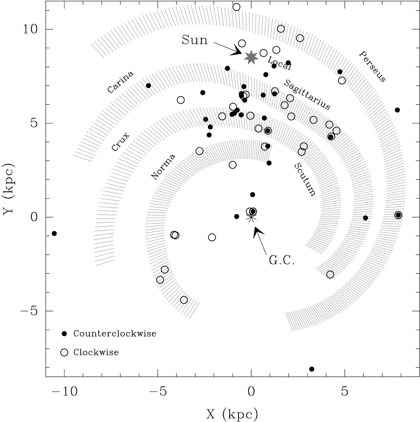
Figure 3: Line-of-sight magnetic field directions deduced from OH maser Zeeman splitting. Seventy-four star-forming regions are plotted, distinguishing 41 with an overall magnetic field oriented in a clockwise sense from 33 with field oriented counterclockwise as viewed from above the Galactic center (i.e., North Galactic Pole). The locations of the Sun and Galactic center are marked. The spiral arms of Taylor & Cordes (1993) are indicated with shading and labelled by their common names.

Assuming that the second and third of the above conditions are satisfied, we can investigate whether there exists a large-scale Galactic magnetic field and what form it takes. The simplest imaginable Galactic field would be a circular field with no reversals in the portion of the disk where massive SFRs are found. Our 74-source sample discussed in §4.5 do not support this model. A plot of the predominant sense of the magnetic field direction (i.e., clockwise or counterclockwise as viewed from the North Galactic Pole) deduced from the OH masers near massive SFRs in this study is shown in Figure 3. For a circular magnetic field configuration in the Milky Way, the sense of the line-of-sight orientation (directed toward or away from the Sun) flips across the $l=0,l=180\arcdeg$ line. Noting this, 41 have magnetic fields directed in a clockwise sense as viewed from the North Galactic Pole and 33 have fields directed in a counterclockwise sense. This does not support a uniform circular field model without reversals. Indeed, it would not be inconsistent with a completely random distribution of magnetic field orientations.

The rough equality of sources with clockwise and counterclockwise fields does not preclude an organized field structure. For instance, the magnetic field could be aligned along either concentric rings or spiral arms but with reversals between the rings or arms. Alternatively, the magnetic field as traced by interstellar OH masers could exhibit organized structure in small (kiloparsec-scale) patches, but not on a Galactic scale. Since our data do not imply a uniform sense of the Galactic magnetic field, a two-point spatial correlation function was calculated on the data in order to test the hypothesis that magnetic field directions of massive SFRs exhibit some degree of correlation over kiloparsec scales. We define the magnetic field orientation of two massive SFRs to be correlated if they are both oriented in a clockwise or counterclockwise Galactic sense. We similarly define a pair to be anti-correlated if the pair consists of one source with a clockwise field and one with a counterclockwise field. The correlation function was defined as the number of pairs of massive SFRs whose fields were correlated in the above sense, divided by the total number of pairs of sources. This function was calculated for a range of intersource distances. Since interpretation of the significance of the correlation function is difficult in isolation, it was compared against the same function evaluated for randomly-generated magnetic-field direction data at the locations of the massive SFRs in our sample. In the random sample, the positions of the maser sources were held fixed, but the line-of-sight field orientation of each source was randomly assigned as toward or away from the Sun. An ensemble of $10^{5}$ such random field distributions was produced. The results are shown in Table 3. The percentages of trial runs showing a lesser and greater degree of correlation do not sum to 100% because some random distributions of magnetic fields produced identical correlation results.

Since the data exhibit roughly equal likelihood of less and more correlation at the 10 or 20 kpc level, our data do not support the original hypothesis of Davies (1974) that there exists a uniform, clockwise Galactic field. On Galactic scales, pulsar rotation measure studies suggest that field reversals exist between spiral arms (e.g., Han et al., 2002; Rand & Lyne, 1994). This would destroy any large-scale correlation on the Galactic scale, as spiral arms with oppositely-oriented magnetic fields would be included at this scale.

On sub-kiloparsec scales there are a number of source complexes in which two nearby massive SFRs have oppositely-oriented line-of-sight magnetic fields. The W49 complex provides a good example of this: G43.148+0.015 (the Zeeman pair is between the sources W49A/R₂ and R₃ in the classification of De Pree, Mehringer, & Goss, 1997) and W49S have fields directed primarily away from the Sun, while the field of W49N is directed toward the Sun. It is possible that this may result from a tangled field geometry associated with multiple cores in the same complex.

Nevertheless, we do note a possible field organization on a $\sim 2$-kpc scale. Indeed, several patches of field coherence at this scale are noticeable in Figure 3. For instance, there is a cluster of sources with clockwise magnetic fields (i.e., oriented toward the Sun) near $(X,Y)=(-4,-3)$ kpc, and another cluster with clockwise fields near $(3,5)$ kpc.

5.3 Rotation Measure Comparison

The structure of the Galactic magnetic field can be studied with rotation measures of Galactic pulsars and extragalactic sources. We find that toward the second and third Galactic quadrants, which contain only six sources, all fields are oriented in the clockwise direction, while the nearest six sources in the first and fourth quadrants are consistent with a counterclockwise field. This agrees with rotation measure studies of the outer Galaxy, which also find an overall clockwise field (Lyne & Smith, 1989; Brown & Taylor, 2001). This also agrees with a reversal inward claimed in other papers from pulsar rotation measure estimates (Simard-Normandin & Kronberg, 1979; Rand & Kulkarni, 1989; Clegg et al., 1992).

In order to compare our results with the Galactic magnetic field deduced from rotation measures, we generated simulated rotation measure data from the line-of-sight magnetic field direction of our OH maser data. Our data consist of measurements of milligauss fields in situ around massive SFRs, while extragalactic rotation measures are line-of-sight integrals predominantly through the microgauss fields of the interstellar medium. We calculated simulated rotation measures along rays of Galactic longitude within the Galactic plane using the line-of-sight field directions from OH masers. The rotation measure $RM$ of radiation coming from a source at a distance $D$ is given by

$$RM=8.1\times 10^{5}~{}\mathrm{rad~{}m^{-2}}\int_{D}^{0}n_{e}\,\mathbf{B\cdot dl},$$

where $n_{e}$ is the electron density in cm^-3, $\mathbf{B}$ is the magnetic field in gauss, and $\mathbf{dl}$ is measured in parsecs. Typical values for these variables in the interstellar medium are $n_{e}\approx 0.03$ cm^-3 (Lyne, Manchester, & Taylor, 1985) and $B_{\|}\approx 2\times 10^{-6}$ G (Manchester, 1974; Simard-Normandin & Kronberg, 1980; Heiles, 1976). Given that magnetic fields implied by Zeeman splitting in massive SFRs exhibit some correlation on a scale of $\lesssim 2$ kpc (see §5.2), we postulated that the magnetic field around a massive SFR indicates the prevailing Galactic magnetic field direction in a sphere of radius $r$ centered at the massive SFR. We adopted $r\sim 0.5$ kpc, which yields a contribution of about 50 rad m^-2 to the rotation measure of a line of sight passing along the diameter of each sphere. Thus, we assigned a rotation measure of $\pm 50$ rad m^-2 to each sphere, depending only on the line-of-sight magnetic field direction in the massive SFR, and summed the rotation measures of the spheres intersected by the ray. For simplicity, each sphere was assumed to contribute $\pm 50$ rad m^-2 to the total rotation measure, regardless of the path length of the ray within the sphere. Note that since the radiation propagates from $D$ to $0$, $\mathbf{dl}$ is oriented toward the Sun, and $\mathbf{B\cdot dl}$ is negative when the magnetic field is oriented away from the Sun. Thus, a positive magnetic field generates a negative rotation measure.

Our simulated rotation measures are plotted in Figure 4 for $r=0.5$ kpc. Features of the plot are not highly sensitive to the value of $r$, but much lower values leave a large volume of the Galactic plane unsampled by our data, while much higher values result in a lot of overlap of the spheres. Superposed atop this plot are extragalactic rotation measures reproduced directly from Figure 9 of Rand & Kulkarni (1989), based on data from Simard-Normandin, Kronberg, & Button (1981). Our data agree reasonably well with the extragalactic rotation measure data. In the second and third Galactic quadrants, our data match the sign of the extragalactic rotation measures. While the extragalactic rotation measures are not generally of consistent sign in the first and fourth quadrants, agreement is found again at $l=15\arcdeg$, where the extragalactic rotation measures are decidedly positive. The simulated rotation measures we deduce from OH Zeeman splitting appear to fit the extragalactic data at least as well as, if not better than, the ring model of Rand & Kulkarni (1989).

5.4 Spiral Arms

In many models, one would expect the Galactic field to be organized along spiral arms. However, investigating whether the Galactic field shows organization on a per-arm basis necessitates assignment of massive SFRs to spiral arms. Based on positions on both a plot of the Galaxy and on the longitude-velocity diagram in Figure 5, most of the sources in our study were assigned to a spiral arm, as listed in Table 6. The above correlation analysis was repeated on the subset of sources associated with each spiral arm, and the results are included in Table 3. For the most part, no obvious correlations exist except for sources assigned to the Norma arm, where 8 of 10 sources (and all 7 in the fourth quadrant) have a magnetic field oriented clockwise with respect to the Galactic center.

As noted above, it is difficult to make strong statements pertaining to field directions in spiral arms. The shape and locations of the spiral arms in the Milky Way are still a matter of debate, and many of the source distances used in this study are kinematic and therefore subject to large enough errors that some could be placed in the wrong arms. Even assuming that the near/far kinematic distance ambiguity has been resolved correctly for all sources, a typical distance error by this method is about 1 kpc. Furthermore, the OH maser velocity may differ from the velocity of the massive SFR, which may in turn deviate quite significantly from uniform circular motion, as discussed in §4.1. Especially near $l=0\arcdeg$, where several spiral arms cross in a longitude-velocity diagram, it is difficult to reliably assign massive SFRs to spiral arms.

5.5 Intra-source Field Reversals

The problem of relating OH Zeeman magnetic field measurements to the Galactic magnetic field can be inverted. Assuming that there exists a large-scale Galactic field, do our results allow us to comment either on whether the magnetic field threading OH maser clumps are related to the (pre-collapse) local Galactic field or on whether intra-source field reversals confuse the issue too much to see conclusive evidence of large-scale field organization?

These are questions that cannot be answered conclusively with the VLA alone, due to its large beam size. For instance, no conclusive Zeeman pairs are found in the 1665 MHz transition in the VLA data for W3(OH). In contrast, Bloemhof, Reid, & Moran (1992) identified 23 Zeeman pairs in the same transition using VLBI. Significant blending of independent maser features within a single VLA beam often renders identification of Zeeman pairs ambiguous, as discussed in §4.5. When Zeeman pairs are identified with VLA resolution, they are often in short supply. We were able to find only one Zeeman pair in many of the massive SFRs shown in Table 1. One pair does not conclusively determine the prevailing magnetic field direction surrounding the region. Even in the simple case, depicted in Figure 6, of a conducting, spherical H II region in a uniform magnetic field, the line-of-sight projection of the magnetic field direction may vary depending on the inclination of the source (Bourke et al., 2001). A numerical simulation was run to estimate the fraction of sources whose line-of-sight magnetic field would be incorrectly inferred owing to projection effects for this simple geometry. Given an ensemble of ideal, spherical H II regions, each with a randomly-oriented prevailing magnetic field direction and a single magnetic field measurement taken locally at a random point on the projection of the sphere (as from a Zeeman pair), the line-of-sight direction of the measured field will be opposite to the line-of-sight direction of the prevailing magnetic field 25% of the time.

Intra-source field reversals have been seen across three of nine massive SFRs that were mapped in the main-line OH transitions with the VLBA: G351.775$-$0.538 (Argon, Reid, & Menten, 2002), W75N, and W75S (unpublished data). Thus, one-third of the population of massive SFRs mapped at milliarcsecond resolution show at least two distinct maser clumps with Zeeman pairs indicating opposite line-of-sight directions. While one might have expected that the magnetic field would be oriented randomly in a massive SFR owing to a complex evolutionary history that “scrambles” the pre-collapse field, massive SFRs with intra-source field reversals still exhibit an organized field structure. More likely, these reversals are a projection effect due to the geometry of the field lines relative to the observer. Still, the ionized sphere model is surely an oversimplification in some cases. For instance, the OH masers around W75N are aligned along two intersecting lines, one running roughly north-south and the other east-west (Baart et al., 1986). Our VLBA data show that the magnetic fields along the north-south line point consistently away from the Sun, while those in the east-west line point consistently toward the Sun. Baart et al. suggest that the masers trace expanding shock waves, while Slysh et al. (2002) claim to have found evidence that the north-south structure is a thin, rotating disk. Whatever the explanation of this source may be, the observed intra-source field reversal is clearly not a simple projection effect in a static environment.

5.6 The Random Component of the Galactic Magnetic Field

Even if the Galactic magnetic field consists of a large-scale field with regular structure, the turbulent field component may hinder clear detection of the pattern. Synchrotron polarization observations suggest that the ratio of field strengths of the regular to turbulent magnetic fields may be between 0.6 and 1.0, with lower values more likely in spiral arms (Beck, 2001). Assuming a uniformly random two-dimensional (in the Galactic plane) orientation of the turbulent component of the magnetic field, the line-of-sight orientation of the total field will be opposite to that of the regular component 8% to 20% of the time for the aforementioned range of field strength ratios. Thus, even if the pre-collapse magnetic field orientation is preserved at sites of OH maser emission, as many as one in five sources could imply a line-of-sight magnetic field opposite to the assumed underlying regular field. On the other hand, Brown & Taylor (2001) present evidence that the random field may be partially aligned with the uniform field, rather than being isotropic. If this is indeed the case, the above estimates of the rate of discrepancy between the magnetic field direction implied by OH Zeeman splitting and the regular field direction may be overly pessimistic. Also, the random component of the Galactic magnetic field may become less significant between interstellar and GMC densities.

6 Conclusions and Further Research

We have found nearly 100 Zeeman pairs of ground-state OH masers using the data from Paper I. Combining these Zeeman pairs with others found in the literature, we have investigated the distribution in the Galactic plane of the line-of-sight orientation of magnetic fields in massive SFRs as deduced from OH maser Zeeman splitting. Our data do not support the original hypothesis of Davies (1974) that the large-scale magnetic field traced by OH masers is uniform in the clockwise sense, nor do we find that the inferred magnetic fields show a uniform direction in each spiral arm.

All six sources in the second and third Galactic quadrants, which are typically 1 or 2 kpc distant, have a magnetic field oriented in the clockwise sense as viewed from the North Galactic Pole, while nearly all nearby sources in the first and fourth quadrants have a magnetic field oriented in the counterclockwise direction. This supports the hypothesis, deduced from pulsar rotation measures, that a reversal of the Galactic-scale magnetic field occurs near the galactocentric radius of the Sun.

Our method for identifying Zeeman pairs in VLA maps of OH masers is limited by the blending of maser components inevitable with a large ($1\arcsec-2\arcsec$) beamsize. The higher resolution of VLBI allows many more maser spots to be detected and Zeeman pairs to be identified unambiguously. The increased detail in VLBI images also allows for the identification of intra-source magnetic field reversals, the interpretation of which may be important both for understanding the conditions of the magnetic field in massive SFRs and for obtaining enough data to rigorously test the hypothesis that the magnetic field deduced from OH maser Zeeman splitting in massive SFRs is correlated with the Galactic magnetic field. To this end, we are in the process of imaging interstellar OH masers with the VLBA. The results will be published in a future paper.

Table 3: Correlation Results

Separation	Pairs of	Percentage of Trial Runs Less/More Correlated
(kpc)	Sources	Overall		Car–Sgr		Cru–Sct		Local		Norma		Perseus
0.5	43	41/	46	14/	65	87/	7	$\cdots$/	$\cdots$	25/	25	0/	63
1.0	111	23/	70	56/	31	14/	72	13/	38	56/	19	0/	63
2.0	324	82/	15	81/	15	76/	19	44/	25	91/	4	19/	44
5.0	1201	52/	45	56/	36	66/	28	0/	38	95/	2	45/	17
10.0	2197	37/	59	42/	48	37/	33	0/	38	89/	2	30/	45
20.0	2664	63/	36	0/	83	37/	33	0/	38	89/	2	49/	18
Number of Sources		74		22		17		5		10		9

Note. — The figures represent the percentage of trial runs for which the correlation function evaluated on the random data were less and more correlated than the actual data. Results to any separation are cumulative; i.e., all pairs of sources with separation less than or equal to a given distance are included in the correlation function results to that distance. The total number of pairs of distinct sources with separation less than the figure in the first column is given in the second column.

Table 4: Sources and Field Directions by Arm

Galactic		Galactic		Distance	Magnetic
Longitude		Latitude		(kpc)	Field	References
Carina–Sagittarius
17.	639	$+0$.	155	2.1	$-$	1
20.	081	$-0$.	135	12.30	$+$	1,7
32.	744	$-0$.	076	2.3	$-$	1,2
34.	258	$+0$.	153	3.8	$+$	1,2,3
35.	024	$+0$.	350	3.1	$+$	1,2
35.	197	$-0$.	743	2.2	$+$	1
35.	577	$-0$.	029	10.50	$-$	1
43.	796	$-0$.	127	3.0	$+$	1,2
45.	071	$+0$.	134	4.7	$+$	1,4,5
45.	122	$+0$.	133	6.0	$-$	1,2,4
45.	465	$+0$.	060	6.0	$+$	1
49.	469	$-0$.	370	6.0	$+$	1,6
49.	488	$-0$.	387	5.5	$+$	1,2,6
285.	26	$-0$.	05	5.7	$-$	2
294.	51	$-1$.	62	1.4	$-$	2
311.	64	$-0$.	38	14.10	$-$	2
344.	581	$-0$.	022	2.0	$-$	1
345.	505	$+0$.	347	2.1	$-$	1,2
345.	699	$-0$.	090	1.6	$-$	1,2
348.	549	$-0$.	978	2.1	$+$	1,2,7
351.	161	$+0$.	697	2.3	$-$	1
351.	416	$+0$.	646	2.0	$+$	1,2,7
Crux–Scutum
5.	886	$-0$.	393	3.8	$+$	1
11.	03	$+0$.	06	3.2	$-$	2
12.	216	$-0$.	117	3.3	$-$	1
12.	680	$-0$.	181	4.0	$-$	1,8
12.	908	$-0$.	259	4.0	$+$	1
28.	199	$-0$.	048	5.7	$+$	1,3
30.	70	$-0$.	06	5.5	$+$	7
323.	459	$-0$.	079	4.1	$-$	2,10
329.	41	$-0$.	46	4.3	$-$	2
331.	34	$-0$.	34	4.7	$-$	7
333.	60	$-0$.	21	3.5	$+$	2
339.	62	$-0$.	12	2.8	$+$	2
341.	219	$-0$.	212	3.2	$-$	1
343.	128	$-0$.	063	3.1	$-$	1
345.	003	$-0$.	224	2.9	$-$	1,2,7
350.	011	$-1$.	341	3.1	$-$	1
359.	138	$+0$.	032	3.1	$+$	1
Local
69.	540	$-0$.	976	1.3	$-$	1,3,9,11
81.	77	$+0$.	60	2.0	$-$	3
106.	80	$+5$.	31	1.4	$+$	3
109.	871	$+2$.	114	0.7	$+$	1,3,12
213.	706	$-12$.	60	0.9	$+$	1
Norma
8.	67	$-0$.	36	4.8	$+$	2
9.	622	$+0$.	195	5.7	$-$	1
10.	624	$-0$.	385	4.8	$-$	1
330.	95	$-0$.	18	5.7	$+$	2,7
336.	36	$-0$.	14	10.30	$+$	2
336.	83	$+0$.	02	10.30	$+$	2
337.	61	$-0$.	06	12.80	$+$	2
337.	71	$-0$.	05	12.20	$+$	2,7
344.	42	$+0$.	05	13.40	$+$	2
350.	11	$+0$.	09	5.8	$+$	2
Perseus
43.	148	$+0$.	015	11.50	$+$	1,2
43.	165	$-0$.	028	11.50	$+$	1
43.	167	$+0$.	010	11.50	$-$	7
70.	293	$+1$.	601	8.3	$-$	1,3,11
75.	782	$+0$.	343	5.0	$+$	11
80.	87	$+0$.	42	4.8	$-$	3
111.	533	$+0$.	757	2.8	$+$	1
133.	946	$+1$.	064	2.2	$+$	1,3,7,13
196.	454	$-1$.	677	2.8	$+$	11
Unassigned
0.	547	$-0$.	852	7.3	$-$	1
0.	666	$-0$.	034	8.2	$+$	1
0.	670	$-0$.	058	8.2	$-$	1
0.	672	$-0$.	031	8.2	$+$	1
40.	42	$+0$.	70	1.2	$-$	1,2
300.	97	$+1$.	15	4.4	$+$	2,7
305.	81	$-0$.	24	3.2	$-$	7
347.	628	$+0$.	149	9.8	$+$	1,2
354.	73	$+0$.	29	8.5	$-$	2
355.	345	$+0$.	146	23.10	$+$	1
359.	436	$-0$.	103	8.2	$+$	1

References. — (1) this paper; (2) Caswell & Vaile 1995; (3) Baudry et al. 1997; (4) Baart & Cohen 1985; (5) Zheng 1997; (6) Gaume & Mutel 1987; (7) Reid & Silverstein 1990; (8) Zheng 1991; (9) Desmurs & Baudry 1998; (10) Caswell & Reynolds 2001; (11) in preparation; (12) Cohen, Brebner, & Potter 1990; (13) García-Barreto et al. 1988

Figure 1: Sample spectra of windows used to find Zeeman pairs. Squares and triangles mark RCP and LCP emission, respectively. Gaussian fits to the lines are shown, and lines and features are numbered for reference. The number in the upper right corner marks the transition frequency, in MHz. (a–d) Windows in G351.775$-$0.538, G032.744$-$0.076, K3$-$50, and G045.465$+$0.047. The 1665 and 1667 MHz windows in (a) and (c) are centered at approximately the same position. The magnetic field and center velocity deduced from Zeeman splitting are shown in (a).

Figure 2: Histogram of the number of Zeeman pairs found with each magnetic field strength, binned by 1 mG. Positive (negative) field strengths represent magnetic fields oriented in the hemisphere away from (toward) the Sun. A best-fit Gaussian is also shown. The $-25.4$ mG pair in G081.871+0.781 is excluded for reasons outlined in §4.3.

Figure 4: Plot of simulated rotation measures generated from magnetic field directions deduced from OH Zeeman splitting. No simulated rotation measures are plotted for Galactic longitudes unsampled by the data of Figures 3 and 5. The dots represent extragalactic rotation measure data as taken from Rand & Kulkarni (1989) at Galactic latitude $b=-15,0$, and $15\arcdeg$. See §5.3 for further details.

Figure 5: Longitude-velocity diagram of magnetic field directions deduced from OH maser Zeeman splitting. Open and filled circles are defined as in Figure 3.

Figure 6: Spherical bubble model of an H II region in a magnetic field. The field is oriented to the upper right and out of the page, inclined $30\arcdeg$ to the line of sight. The arrows at a and b represent the local magnetic field at two points as might be deduced from Zeeman splitting. The line-of-sight projection of the magnetic field is out of the page outside the dotted curve (as at a) and into the page inside the curve (as at b). In the limiting cases of the magnetic field aligned along (perpendicular to) the line of sight, the line-of-sight direction of the field is reversed over none (half) of the projected area of the sphere. For a uniform distribution of magnetic field directions intersecting a sphere at all possible angles, on average the line-of-sight direction of the magnetic field is reversed over $25\%$ of the area of the projected sphere.

References

- Argon, Reid, & Menten (2000) Argon, A. L., Reid, M. J., & Menten, K. M. 2000, ApJS, 129, 159 (Paper I)
- Argon, Reid, & Menten (2002) Argon, A. L., Reid, M. J., & Menten, K. M. 2002, in IAU Symposium 206, Cosmic MASERs: From Protostars to Blackholes, ed. V. Migenes and M. J. Reid (San Francisco: ASP), 367
- Baart et al. (1986) Baart, E. E., Cohen, R. J., Davies, R. D., Rowland, P. R., & Norris, R. P. 1986, MNRAS, 219, 145
- Baart & Cohen (1985) Baart, E. E., & Cohen, R. J. 1985, MNRAS, 213, 641
- Baudry et al. (1997) Baudry, A., Desmurs, J. F., Wilson, T. L., & Cohen, R. J. 1997, A&A, 325, 255
- Beck (2001) Beck, R. 2001, Space Sci. Rev., 99, 243
- Bloemhof, Reid, & Moran (1992) Bloemhof, E. E., Reid, M. J., & Moran, J. M. 1992, ApJ, 397, 500
- Brown & Taylor (2001) Brown, J. C., & Taylor, A. R. 2001, ApJ, 563, L31
- Bourke et al. (2001) Bourke, T. L., Myers, P. C., Robinson, G., & Hyland, A. R. 2001, ApJ, 554, 916
- Campbell & Thompson (1984) Campbell, B., & Thompson, R. I. 1984, ApJ, 279, 650
- Caswell (2001) Caswell, J. L. 2001, MNRAS, 326, 805
- Caswell & Reynolds (2001) Caswell, J. R., & Reynolds, J. E. 2001, MNRAS, 325, 1346
- Caswell & Vaile (1995) Caswell, J. L., & Vaile, R. A. 1995, MNRAS, 273, 328
- Clegg et al. (1992) Clegg, A. W., Cordes, J. M., Simonetti, J. M., & Kulkarni, S. R. 1992, ApJ, 386, 143
- Cohen, Brebner, & Potter (1990) Cohen, R. J., Brebner, G. C., & Potter, M. M. 1990, MNRAS, 246, 3P
- Davies (1974) Davies, R. D. 1974, in IAU Symposium 60, Galactic Radio Astronomy, ed. F. J. Kerr and S. C. Simonson III (Dordrecht:Reidel), p. 275
- De Pree, Mehringer, & Goss (1997) De Pree, C. G., Mehringer, D. M., & Goss, W. M. 1997, ApJ, 482, 307
- Desmurs & Baudry (1998) Desmurs, J. F., & Baudry, A. 1998, A&A, 340, 521
- Dickel, Dickel, & Wilson (1978) Dickel, J. R., Dickel, H. R., & Wilson, W. J. 1978, ApJ, 223, 840
- Fish et al. (2002) Fish, V. L., Reid, M. J., Argon, A. L., & Menten, K. M. 2002, in IAU Symposium 206, Cosmic MASERs: From Protostars to Blackholes, ed. V. Migenes and M. J. Reid (San Francisco: ASP), 371
- Fish et al. (2003) Fish, V. L., Reid., M. J., Wilner, D. J., & Churchwell, E. 2003, ApJ, 587, 701
- Forster & Caswell (1989) Forster, J. R., & Caswell, J. L. 1989, A&A, 213, 339
- García-Barreto et al. (1988) García-Barreto, J. A., Burke, B. F., Reid, M. J., Moran, J. M., Haschick, A. D., & Schilizzi, R. T. 1988, ApJ, 326, 954
- Gaume & Mutel (1987) Gaume, R. A., & Mutel, R. L. 1987, ApJS, 65, 193
- Han et al. (2002) Han, J. L., Manchester, R. N., Lyne, A. G., & Qiao, G. J. 2002, ApJ, 570, L17
- Haschick & Ho (1983) Haschick, A. D., & Ho, P. T. P. 1983, ApJ, 267, 638
- Heiles (1976) Heiles, C. 1976, ARA&A, 14, 1
- Hofner et al. (1994) Hofner, P., Kurtz, S., Churchwell, E., Walmsley, C. M., & Cesaroni, R. 1994, ApJ, 429, L85
- Humphreys (1978) Humphreys, R. M., 1978, ApJS, 38, 309
- Lyne, Manchester, & Taylor (1985) Lyne, A. G., Manchester, R. N., & Taylor, J. H. 1985, MNRAS, 213, 613
- Lyne & Smith (1989) Lyne, A. G., & Smith, F. G. 1989, MNRAS, 237, 533
- Manchester (1974) Manchester, R. N. 1974, ApJ, 188, 637
- Mouschovias (1976) Mouschovias, T. C. 1976, ApJ, 207, 141
- Rand & Kulkarni (1989) Rand, R. J., & Kulkarni, S. R. 1989, ApJ, 343, 760
- Rand & Lyne (1994) Rand, R. J., & Lyne, A. G. 1994, MNRAS, 268, 497
- Reid et al. (1980) Reid, M. J., Haschick, A. D., Burke, B. F., Moran, J. M., Johnston, K. J., & Swenson, G. W., Jr. 1980, ApJ, 239, 89
- Reid et al. (1999) Reid, M. J., Readhead, A. C. S., Vermeulen, R. C., & Treuhaft, R. N. 1999, ApJ, 524, 816
- Reid & Moran (1981) Reid, M. J., & Moran, J. M. 1981, ARA&A, 19, 231
- Reid, Myers, & Bieging (1987) Reid, M. J., Myers, P. C., & Bieging, J. H. 1987, ApJ, 312, 830
- Reid & Silverstein (1990) Reid, M. J., & Silverstein, E. M. 1990, ApJ, 361, 483
- Scoville et al. (1987) Scoville, N. Z., Yun, M. S., Clemens, D. P., Sanders, D. B., & Waller, W. H. 1987, ApJS, 63, 821
- Simard-Normandin & Kronberg (1979) Simard-Normandin, M., & Kronberg, P. P. 1979, Nature, 279, 115
- Simard-Normandin & Kronberg (1980) Simard-Normandin, M., & Kronberg, P. P. 1980, ApJ, 242, 74
- Simard-Normandin, Kronberg, & Button (1981) Simard-Normandin, M., Kronberg, P. P., & Button, S. 1981, ApJS, 45, 97
- Slysh et al. (2002) Slysh, V. I., Migenes, V., Val’tts, I. E., Lyubchenko, S. Yu., Horiuchi, S., Altunin, V. I., Fomalont, E. B., & Inoue, M. 2002, ApJ, 564, 317
- Sofue et al. (1986) Sofue, Y., Klein, U., Beck, R., & Wielebinski, R. 1986, Ap&SS, 119, 191
- Taylor & Cordes (1993) Taylor, J. H., & Cordes, J. M. 1993, ApJ, 411, 674
- Wilson (1974) Wilson, T. L. 1974, A&A 31, 83
- Zheng (1991) Zheng, X. 1991, ChA&A, 15, 219
- Zheng (1997) Zheng, X. 1997, ChA&A, 21, 182
- Zheng, Reid, & Moran (2000) Zheng, X., Reid, M. J., & Moran, J. M. 2000, A&A, 357, L37