An $\alpha$-stable approach to the study of the $P(D)$ distribution of unresolved point sources in CMB sky maps

We present a new approach to the statistical study and modelling of number counts of faint point sources in astronomical images, i.e. counts of sources whose flux falls below the detection limit of a survey. The approach is based on the theory of $\alpha$-stable distributions. We show that the non-Gaussian distribution of the intensity fluctuations produced by a generic point source population – whose number counts follow a simple power law – belongs to the $\alpha$-stable family of distributions. Even if source counts do not follow a simple power law, we show that the $\alpha$-stable model is still useful in many astrophysical scenarios. With the $\alpha$-stable model it is possible to totally describe the non-Gaussian distribution with a few parameters which are closely related to the parameters describing the source counts, instead of an infinite number of moments. Using statistical tools available in the signal processing literature, we show how to estimate these parameters in an easy and fast way. We demonstrate that the model proves valid when applied to realistic point source number counts at microwave frequencies. In the case of point extragalactic sources observed at CMB frecuencies, our technique is able to successfully fit the $P(D)$ distribution of deflections and to precisely determine the main parameters which describe the number counts. In the case of the Planck mission, the relative errors on these parameters are small either at low and at high frequencies. We provide a way to deal with the presence of Gaussian noise in the data using the empirical characteristic function of the $P(D)$. The formalism and methods here presented can be very useful also for experiments in other frequency ranges, e.g. X-ray or radio Astronomy.

1 Introduction

The study of intensity (or temperature) fluctuations in the Cosmic Microwave Background (CMB) radiation has become one of the milestones of modern cosmology due to two main reasons. On the one hand, the angular power spectrum of the fluctuations allow us to place tight constraints on the fundamental cosmological parameters (see, e.g., Bennett et al. 2003a ). For a recent review on the study of CMB anisotropies, see Hu & Dodelson (hu (2002)). On the other hand, the study of the different physical sources (foregrounds) that contribute to the incoming radiation at microwave wavelengths has a great scientific relevance in itself (De Zotti et al. zotti2 (1999)). Therefore, a great deal of effort has been devoted to the task of separating the different components that are present in CMB maps. In general, component separation techniques take advantage of the statistical behaviours of each component to distinguish among them. Hence, it is important to have good statistical models for each of the components under study.

Among the different foregrounds that appear in CMB observations, extragalactic point sources (EPS), i.e. individual galaxies whose typical angular size is much smaller than the observing beam width (hence the name ‘point sources’) are especially difficult to deal with. The galaxies that contribute to the observed total signal are very diverse, corresponding to objects at different redshifts and with different physical properties. This makes it impossible to establish a single spectral behaviour for all of them, thus hampering the performance of methods that use multi-frequency observations to achieve an efficient component separation. The spatial distribution of faint EPS is roughly uniform across the sky even in presence of source clustering. Therefore, Galactic cuts useful to avoid Galactic foregrounds such as synchrotron, dust and free-free emission, are not applicable to avoid EPS contamination.

EPS contamination occurs when a set of point-like sources with intensities distributed following a general law, usually modelled as a power law, is observed by a detector using a given instrumental response. The final signal is a mixing in which the brightest sources are still individually detectable over a ‘confusion noise’ generated by the contributions of faint, unresolved sources; this situation is very common in astronomical images and it has been studied first at radio and X-ray frequencies. The intensity (or temperature) distribution given by unresolved sources is strongly non-Gaussian and shows long positive tails. This kind of behaviour is known in the signal processing literature as ‘impulsive noise’.

The effect of the confusion noise is two fold: on one hand the mean value of this noise is positive, producing a ‘source monopole’ (integrated extragalactic background) that has to be summed up to the other components and, on the other hand, it gives rise to small scale intensity fluctuations. At microwave frequencies, the fluctuations generated by undetected sources can severely hamper the detection of true CMB anisotropies (Franceschini et al. franceschini1 (1989)). Recently, Toffolatti et al. (T98 (1998); hereafter T98) presented a detailed analysis of the effect of point sources on CMB anisotropy maps. By exploiting a cosmological evolution model for radio and far-IR selected sources, they made precise predictions on source counts, on confusion noise and on the angular power spectrum due to undetected sources. In particular, they showed that the contribution of EPS will be very relevant at the lower and higher frequency channels of the future ESA Planck mission (Mandolesi et al. mandolesi (1998); Puget et al. puget (1998)). As for radio source counts, the predictions of T98 have been confirmed by the first year data of the NASA Wilkinson Microwave Anisotropy Probe (WMAP) mission (Bennett et al. 2003b ), al least up to frequencies of $\sim 30-40$ GHz. The WMAP all sky catalogue of bright extragalactic sources (Bennett et al. 2003b ) consists of 208 objects with fluxes $S>0.9\div 1$ Jy on a sky area of 10.38 sr ($|b^{II}|>10^{\circ}$) whereas the T98 model predicts 270-280 sources at 30 GHz in the same area with an average offset of $\sim 0.75$ between observed and predicted number of extragalactic sources. Moreover, the distribution of energy spectral indexes (i.e. $a$, $S\propto\nu^{-a}$) of sources in the WMAP sample peaks around $a=0.0$, which is exactly the mean value of the energy spectral index adopted in T98 for “flat”–spectrum sources, i.e. the dominant source population at these frequencies (the fraction of “steep”–spectrum sources being $\sim 10\div 15\%$). It is also noticeable that the brightest source detected by WMAP has a flux density of $S\simeq 25$ Jy which, again, corresponds to the flux value for which the T98 model predicts 1 source all over the sky. Another important result confirming the estimates of the T98 cosmological evolution model is that a good agreement is currently found between predictions based on that model and data on the excess angular power spectrum at small angular scales as well as on the angular bispectrum detected in the WMAP Q and V bands (Komatsu et al. komatsu (2003), Argüeso et al. paco (2003)). Two other independent samples of extragalactic sources at 31 and 34 GHz – from CBI (Mason et al. mason (2003)) and VSA (Taylor et al. taylor (2003)) experiments, respectively – show that the T98 model correctly predicts number counts down to, at least, $S\simeq 10$ mJy. Therefore, we can confidently use the T98 model for simulating Poisson distributed EPS in CMB sky maps, at least up to 50-100 GHz. At higher frequencies, more recent models can give a better fit to current data on source counts (see section 5.1.2). As the outcomes of the methods to be presented here are model independent, we still use the T98 model throughout the paper.

The current low sensitivity of detectors at CMB frequencies makes it impossible to test directly model counts down to fainter fluxes. On the other hand, more information on counts of faint sources, i.e. sources with fluxes fainter than the detection threshold of a given experiment, can be extracted by the analysis of the intensity fluctuations of point sources. The probability density function pdf of fluctuations due to undetected point sources, as a first step to the modelling of the confusion noise, has been studied since the middle of the last century (Scheuer scheuer1 (1957), scheuer2 (1974); Condon condon (1974); Hewish hewish (1961)). These works have shown that it is possible to find analytical expressions for the characteristic function of the pdf (in Fourier space), but not for the pdf in the real space. This fact has hampered the development of specific statistical tools to deal with the EPS confusion noise.

In analysing a sky map there are two traditional ways of determining the main statistical properties of a given source population. One possibility is to detect the brightest point sources in a given data set, e.g. using a linear filter to detect them, and then obtain parameters such as the number counts, their slope, etc. For example, Vielva et al. (vielva (2003)) detect point sources in realistic Planck simulations using a Mexican Hat Wavelet technique and compare the number of detections with the input number counts, which correspond to the T98 model. The other possibility is to directly study the pdf of the confusion noise which, in general, is mixed with the signal coming from CMB and the other foregrounds plus instrumental noise. This is generally performed using statistical indicators such as the moments up to a certain degree (see, e.g., Rubiño-Martín & Sunyaev rubi (2003) and Pierpaoli pierpaoli (2003)) or the non-Gaussianity of the wings. A computationally more complex way is to calculate numerically the theoretical pdf assuming some model for source counts and trying to fit it to the data (Condon & Dressel condon2 (1978); Franceschini et al. franceschini1 (1989)). Anyway, the lack of an analytical form for the pdf makes difficult to establish the optimal estimator of its parameters. In particular, it is not clear how many moments are necessary to characterise the pdf (in principle, infinite of them) or which ones are more appropriate for extracting information (it is generally assumed, on the basis of mere intuition, that the third order moment should be one of them).

In this paper we will focus on the application of a novel formalism, the $\alpha$-stable distributions, to model the pdf of the intensity fluctuations due to point extragalactic sources. $\alpha$-stable distributions are known to be very efficient in modelling impulsive noise. They have a number of interesting mathematical properties that make them very attractive; in particular, it is possible to show that the Gaussian distribution is a special case of the more general class of $\alpha$-stable distributions and that $\alpha$-stable distributions satisfy a generalised form of the central limit theorem. Moreover, in this work we show that the pdf of a theoretical power law representing the number counts of extragalactic sources observed with a filled-aperture instrument must follow exactly an $\alpha$-stable distribution. The great advantage is that $\alpha$-stable distributions are completely described by a small number of parameters, what makes them relatively easy to deal with. Optimal techniques already existent in the signal processing literature are easy to adapt to directly extract the main parameters of the source number counts (namely, the slope of the number counts power law and its normalisation) without having to resort to clumsy statistics. Finally, the methods can be generalised for dealing with mixtures of signals, as is the case when the EPS population is added to Gaussian instrumental noise.

Therefore, this work aims at four objectives: first, we will demonstrate that a generic extragalactic point source population whose number counts follow a power law inevitably leads, when observed with a filled-aperture instrument, to a pdf which belongs to the family of $\alpha$-stable distributions. Then, we will devote some time to introduce the $\alpha$-stable distributions to the community, reviewing their main properties and giving the necessary references for further reading. In a third part of this paper we will discuss how $\alpha$-stable distributions can be used to model and study more realistic cases, such as the truncated power law, and we will show that the model is a good approximation for most cases of astronomical interest. Finally, we will discuss the case in which other astronomical or instrumental signals –such as the Cosmic Microwave Background (CMB) radiation or instrumental noise– are mixed with the point sources. In that case, a method will be suggested that is able to obtain the parameters of the point source deflection distribution even in presence of ‘contamination’.

The structure of this paper is as follows: in Sect. 2 we review the basics of the derivation of the characteristic function of the deflection distribution. In Sect. 3 the $\alpha$-stable distributions and their main properties are introduced. Section 4 deals with the extraction of the physical parameters of the EPS population using the $\alpha$-stable formalism. In Sect. 5 we study the application of the formalism to more realistic source models, using as an example the T98 point source model. Parameter estimation of $\alpha$-stable processes mixed with Gaussian noise is considered in section 6. A few considerations about the implementation of these techniques for the future Planck mission are given in section 7. Finally, in Sect. 8 we summarise our conclusions.

2 Source counts and the deflection probability function $P(D)$

Let us consider a population of EPS whose differential number counts can be described in a power law form:

$$n(S)=kS^{-\eta},\ \ \ S>0,$$ (1)

where $\eta$ is the slope of the differential counts power law, $k$ is called its normalisation and $S$ is the intrinsic flux. The sources are assumed to be distributed uniformly across the sky and, at the moment, we will assume that eq. (1) holds for all $S>0$. The sources are now observed with an instrument whose angular response is $f(\theta,\phi)$, not necessarily normalised to unity at the peak. Then, the mean number of sources responses of intensity $x=f(\theta,\phi)S$ in the beam at any time is

$$R(x)=\int n\left[\frac{x}{f(\theta,\phi)}\right]\frac{d\Omega}{f(\theta,\phi)}.$$ (2)

Substituting eq. (1) into eq. (2) we have that

$$R(x)=k\Omega_{e}x^{-\eta},$$ (3)

where

$$\Omega_{e}=\int\left[f(\theta,\phi)\right]^{\eta-1}d\Omega$$ (4)

is a geometrical factor called effective beam solid angle. Let us now define the deflection $D$ as the fluctuation field that is observed, that is $D=I-\langle I\rangle$, where $I$ is the intensity at a given point (time) and $\langle I\rangle$ is its average value, i.e. $\langle I\rangle$ represents the extragalactic background due to undetected EPS. Let us define the characteristic function of a given function $g(x)$ as

$$G(w)=\int_{-\infty}^{\infty}g(x)\ e^{-iwx}dx.$$ (5)

Scheuer (scheuer1 (1957)) showed that the characteristic function of the probability distribution $P(D)$ is related to the characteristic function of $R(x)$ through

$$\psi(w)=\exp\left[r(w)-r(0)\right],$$ (6)

where $\psi(w)$ and $r(w)$ are the characteristic functions of $P(D)$ and $R(x)$, respectively.

Using eqs. (3), (5) and (6) it is possible to calculate the characteristic function $\psi(w)$. This calculation has been performed by several authors, including Scheuer (scheuer1 (1957)), Condon (condon (1974)), Barcons (barcons (1992)) and Franceschini et al. (franceschini1 (1989)). After some effort we obtain

$$\psi(w)=\exp\left\{i\mu w-\gamma\left|w\right|^{\alpha}\left[1+i\beta\textrm{sgn}(w)\tan\left(\frac{\alpha\pi}{2}\right)\right]\right\},$$ (7)

where the parameters $\alpha$, $\beta$, $\gamma$ and $\mu$ relate to the physical parameters of the EPS and of the detector through

$$\alpha=\eta-1,$$ (8)

$$\beta=\frac{1}{\pi}\Gamma\left(\frac{1+\alpha}{2}\right)\Gamma\left(\frac{1-\alpha}{2}\right)\cos\left(\frac{\alpha\pi}{2}\right)=1,$$ (9)

$$\gamma=\frac{\pi^{3/2}k\Omega_{e}}{2^{\alpha+1}\Gamma\left(\frac{\alpha+1}{2}\right)\Gamma\left(\frac{\alpha+2}{2}\right)\sin\left(\frac{\alpha\pi}{2}\right)},$$ (10)

$$\mu=\frac{k\Omega_{e}}{1-\alpha}\lim_{a\rightarrow 0^{+}}a^{1-\alpha}.$$ (11)

The terms in eq. (7) have been arranged in this way for a reason that will be clear in the following. The second equality in eq. (9) is due to the properties of the gamma function (Abramowitz abramowitz (1971)), and as far has we know it hasn’t been noticed before now. The previous equations are valid for $1<\eta<3$. For $\eta>2$ the parameter $\mu$ is not finite, a situation equivalent to the classic Olbers’ paradox in which the observed integrated flux density is infinite in all directions of the sky.

Equation (7) has an important drawback: to obtain the pdf of the deflections, $P(D)$, it is necessary to make the inverse Fourier transform of $\psi(w)$ which, in general, cannot be evaluated analytically. Although it can be performed numerically, the computational cost can be high if many different realisations are needed for a particular task, and numerical integration does not lead to closed form solutions. Instead of doing that, let us see what can be learnt from the characteristic function itself. As we will see in the next section, eq. (7) corresponds exactly to the actual definition of a family of distributions that is known in the statistical signal processing literature as $\alpha$-stable distributions.

3 A short introduction to $\alpha$-stable distributions

In this section we will make a summary introduction to the $\alpha$-stable distributions, in order to clarify some concepts that will be used later. Starting from the particular case of the EPS $P(D)$ characteristic function in eq. (7), that we will see that belongs to the $\alpha$-stable family, we will proceed to a more general description of $\alpha$-stable phenomena that could be useful for astronomers.

The characteristic function in eq. (7) corresponds to a pdf that in general should be calculated numerically and that exhibits heavier tails than a Gaussian distribution. In Fig. 1 the pdf corresponding to eq. (7) with $\beta=1$, $\gamma=1$ and three different values of $\alpha$ (1.1, 1.5 and 1.9) are shown. The presence of heavy tails mean that ‘glitches’ are more likely to occur than in the Gaussian case. In the signal processing literature, probability density functions with tails heavier than the Gaussian are called to be impulsive. A process is impulsive if it takes large values that significantly deviates from the mean value with non-negligible probability. These large values often appear as conspicuous outlayers. Impulsive processes are ubiquitous in many ‘real-world’ problems, from atmospheric noise caused by electric discharges to financial time series data. For more information on impulsive noise, see Kuruoğlu (ercan1 (1998)). A great deal of effort has been done to model impulsive processes; is in that context that the $\alpha$-stable distributions have experienced popularity. Other models that deal with impulsive processes, such as the Middleton’s (Middleton middleton (1977)), Cauchy and Student-T models, are very case specific while the $\alpha$-stable model is general and has a strong theoretical justification.

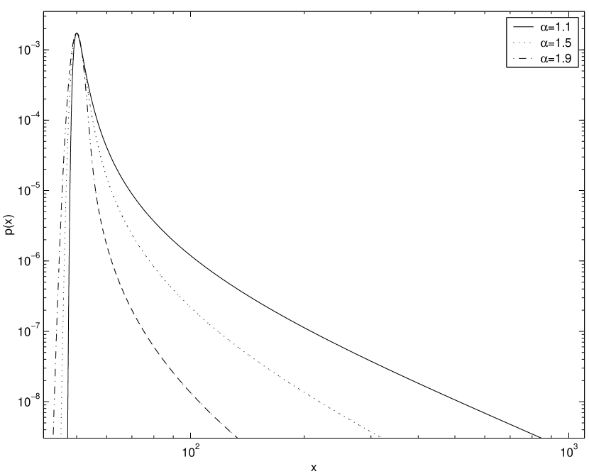
Figure 1: Probability density functions corresponding to three different $\alpha$-stable models. The parameters of the $\alpha$-stable are $\beta=1$, $\gamma=1$ and $\alpha=$ 1.1 (solid line), 1.5 (dotted line) and 1.9 (dot-dashed line). For an easier comparison among them, the $\mu$ parameter of each distribution has been set so that the maximum of all the pdfs coincide at the arbitrary value $x=50$. The pdf becomes more impulsive (departs more from the Gaussian case) as $\alpha$ decreases.

Although $\alpha$-stable distributions were known from the beginnings of XX^th century (Lévy levy (1925)), it was not until the work of Shao & Nikias (shao (1993)) that they received more interest in the signal processing literature. The $\alpha$-stable distribution is a generalisation of the Gaussian distribution that furnishes tractable examples of impulsive behaviour and allows us to describe such behaviour by means of a small number of parameters. The $\alpha$-stable distributions are usually defined by their characteristic function:

$$\psi(w)=\exp\left\{i\mu w-\gamma\left|w\right|^{\alpha}B_{w,\alpha}\right\},$$ (12)

$$B_{w,\alpha}=\left\{\begin{array}[]{ll}\left[1+i\beta\textrm{sgn}(w)\tan\left(\frac{\alpha\pi}{2}\right)\right]&\textrm{if $\alpha\neq 1$}\\ \left[1+i\beta\textrm{sgn}(w)\frac{2}{\pi}\log{\left|w\right|}\right]&\textrm{if $\alpha=1$}\\ \end{array}\right.$$ (13)

where $-\infty<\mu<\infty,\ \gamma>0,\ 0<\alpha\leq 2$ and $-1\leq\beta\leq 1$. The four parameters $\mu,\ \alpha,\ \beta$ and $\gamma$ uniquely and completely determine the stable distribution. The meanings of these parameters are:

1. The parameter $\alpha$ is called the characteristic exponent and sets the degree of impulsiveness of the distribution. For $\alpha=2$ the distribution corresponds to the Gaussian distribution and, as $\alpha$ decreases the distribution gets more and more impulsive. Another particular case is when $\alpha=1$ and $\beta=0$, that corresponds to the Cauchy distribution. For $\alpha\notin(0,2]$ the inverse Fourier transform of $\psi(w)$ is not positive-definite and hence is not a proper probability density function.

2. The parameter $\beta$ is called symmetry parameter and determines the skewness of the distribution. Totally symmetric distributions have $\beta=0$, whereas $\beta=\pm 1$ corresponds to totally skewed distributions.

3. The parameter $\gamma$ is called scale parameter. It is a measure of the spread of the samples from a distribution around the mean. When $\alpha=2$ we get the Gaussian case and then $\gamma=\sigma_{G}^{2}/2$, where $\sigma_{G}$ is the dispersion of the Gaussian.

4. The parameter $\mu$ is called location parameter and basically corresponds to a shift in the x-axis of the pdf. For a symmetric ($\beta=0$) distribution, $\mu$ is the mean when $1<\alpha\leq 2$ and the median when $0<\alpha\leq 1$.

As it can be seen, the first case in eqs. (12) and (13), $\alpha\neq 1$, has exactly the same expression as eq. (7). For simplicity, through this paper we are not going to consider the case $\alpha=1$, as it corresponds to a single point (of zero measure) in the interval $(0,2]$.

Going back to the expressions in Sect. 2, we see that eq. (7) held when $1<\eta<3$, that is, when $0<\alpha<2$. As $k$ and $\Omega_{e}$ are positive in eq. (10) and $0<\alpha<2$ we have that $\gamma>0$. By eq. (9) we know that $\beta=1$. Therefore, eq. (7) is exactly the characteristic function of an $\alpha$-stable distribution with maximum positive skew.

The fact that a population of point sources that are distributed in intensity following a power law and that are observed with a pencil-beam instrument produce an $\alpha$-stable distribution of deflections is very convenient. The $\alpha$-stable representation offers several advantages:

1. Simplicity: a non-Gaussian distribution that follows eq. (13) can be completely described by only four parameters, instead of an infinite number of moments.

2. Mathematical justification: $\alpha$-stable distributions include as a particular case the Gaussian distribution, and share with it many desirable properties. First, they satisfy the generalised central limit theorem which states that the limit distribution on infinitely many i.i.d. random variables, possibly with infinite variance distribution, is a stable distribution (Feller feller (1966)). Therefore, the use of $\alpha$-stable distributions is strongly justified from the theoretical point of view, as they are able to describe a wider range of data which might not satisfy the classical central limit theorem. In second place, $\alpha$-stable distributions have the stability property: the output of a linear system in response to $\alpha$-stable inputs is again $\alpha$-stable and various aspects of linear system theory developed for Gaussian signals extend directly to the case of signals with $\alpha$-stable distribution. For more information on the mathematical foundation of stable distributions, see Samorodnitsky & Taqqu (samorodnitsky (1994)) and references therein.

3. Ubiquity: $\alpha$-stable can be shown to be the limit distribution of natural noise processes under realistic assumptions pertaining to their generation mechanism and propagation conditions (Nikias & Shao nikias (1995)). They agree with empirical data extremely well in so different situations as noise in telephone lines, atmospheric noise, radio networks, radar systems, financial time series, etc. Even in cases in which there is not a strong theoretical or physical evidence that an expression such as eq. (13) holds, $\alpha$-stable representation still provides a good modelling of many processes. For example, later in this work we will show that the $\alpha$-stable model works well even when the source counts do not follow a pure power law, or when the power law is cut at a certain flux limits.

There is another advantage in the $\alpha$-stable formulation: they have been thoroughly studied in the literature, and their properties are well understood. Until recently the $\alpha$-stable distributions were generally avoided for two main reasons: first, the probability distribution has not a closed form in real space (except for the particular cases of the Gaussian, Cauchy and Pearson distributions). This greatly hamper the development of statistical signal processing techniques such as maximum-likelihood and Bayesian estimates. The second one is that the non-Gaussian $\alpha$-stable distributions have infinite variance (and, in some cases, as we have seen in the case of EPS and $\eta>2$, a $\mu$ parameter which is not finite), and it was considered that $\alpha$-stable distributions cannot be physical. But the same objection applies to a very well-known process, the white noise, but it is however universally used in all fields of science and engineering. The variance of the theoretical white noise is not finite, but this doesn’t stop scientists to use it as an accurate and useful model for real, finite processes. In the same way, $\alpha$-stable distributions have been shown to provide excellent fit to a very wide class of processes observed both in the natural world as well as many artificial systems. In the last few years a great deal of effort has been carried out in the signal processing field to overcome the two drawbacks above mentioned. Now there is a plethora of available methods to perform statistical inference on $\alpha$-stable environments. In this work we will focus on the application of existent techniques for $\alpha$-stable parameter extraction in order to obtain optimal estimators of the parameters describing the differential counts of the EPS population, namely the slope $\eta$ and the normalisation $k$.

4 Point source parameter extraction using $\alpha$-stable distributions

After the general discussion of $\alpha$-stable distributions presented in the last section, let us now return to the particular case of the $P(D)$ and its $\alpha$-stable distribution posed by eqs. (7) to (11).

According to equations (8) to (11), the usual parameters describing the differential counts of the EPS population are directly related with the parameters of the $\alpha$-stable distribution of observed deflections. In particular, using equations (8) and (10) we have that

$$\eta=\alpha+1,$$ (14)

$$k=\gamma\frac{2^{\alpha+1}\Gamma\left(\frac{\alpha+1}{2}\right)\Gamma\left(\frac{\alpha+2}{2}\right)\sin\left(\frac{\alpha\pi}{2}\right)}{\pi^{3/2}\Omega_{e}}.$$ (15)

Therefore, it suffices to estimate the parameters $\alpha$ and $\gamma$ to directly estimate $\eta$ and $k$. Over the past years a number of efficient estimators for the parameters of $\alpha$-stable distributions have been developed. Unfortunately, most of them consider only the estimate in the case of symmetric $\alpha$-stable distributions ($\beta=0$), due to the fact that is the most common case in many signal processing applications. On the other hand, very recently Kuruoğlu (ercan2 (2001)) introduced a number of density parameter estimators for skewed $\alpha$-stable distributions. The simplest estimators are based on the following idea: let us consider an $\alpha$-stable distribution with parameters $\alpha$, $\beta$, $\gamma$ and $\mu$, and denote it by $S_{\alpha}(\beta,\gamma,\mu)$. If $X_{i},\ i=1,\ldots,N$ is the sequence of data, it is easy to show that very simple manipulations of the data can be performed in order to produce centred, deskewed or symmetrised sequences, respectively:

$$X_{k}^{C} = X_{3k}+X_{3k+1}-2X_{3k-2}$$ (16)

$$\sim S_{\alpha}\left(\left[\frac{2-2^{\alpha}}{2+2^{\alpha}}\right]\beta,\left[2+2^{\alpha}\right]\gamma,0\right)$$

$$X_{k}^{D} = X_{3k}+X_{3k+1}-2^{1/\alpha}X_{3k-2}$$ (17)

$$\sim S_{\alpha}\left(0,4\gamma,\left[2-2^{1/\alpha}\right]\mu\right)$$

$$X_{k}^{S} = X_{2k}-X_{2k-1}$$ (18)

$$\sim S_{\alpha}(0,2\gamma,0).$$

In the previous equations, the symbol $\sim$ means equality in distribution and therefore they must be regarded as exact equations, not approximations. The only caveat is that they work only if the samples $X_{nk}$, $X_{nk-1}$, etc are independent random variables. Due to the correlations introduced by the beam at small scales, this is not true if the samples that appear in each individual summation are neighbours. Fortunately, at scales larger than a few arcmin, where the effect of the beam is negligible, statistical independence is satisfied. To ensure the validity of equations (16) to (18) it is enough to randomly shuffle the data before operating. Since in this paper we do only a first order statistical modelling –we deal with the ensemble of data rather than a time or space series– this has no other effect on the methods we present here apart from guaranteeing the good behaviour of the previous equations.

Once the distribution is conveniently centred, deskewed or symmetrised, the techniques for symmetric $\alpha$-stable parameter estimate can be applied. Kuruoğlu (ercan2 (2001)) describes several groups of techniques adequate for such task: fractional lower order moment (FLOM) methods, logarithmic moment methods and extreme value methods. Other useful methods are based on the study of the empirical characteristic function of the data. Kuruoğlu (ercan2 (2001)) studied the comparison between the different techniques and showed that both FLOM and logarithmic methods are very efficient in general. In this work we are going to use the logarithmic method, as it is easier to implement.

4.1 Logarithmic moments estimators

Let $X$ be a set of data distributed following an $\alpha$-stable $\sim S_{\alpha}(\beta,\gamma,0)$. Let us define the logarithmic moments of the distribution

$$L_{1}=\mathbf{E}\left[\log\left|\mathit{X}\right|\right],$$ (19)

$$L_{2}=\mathbf{E}\left[\left(\log\left|\mathit{X}\right|-\mathbf{E}\left[\log\left|\mathit{X}\right|\right]\right)^{2}\right],$$ (20)

where $\mathbf{E}$ is the usual estimator operator. It can be shown (Kuruoğlu ercan2 (2001)) that

$$L_{1} = \psi_{0}\left(1-\frac{1}{\alpha}\right)+\frac{1}{\alpha}\log\left|\frac{\gamma}{\cos\theta}\right|,$$ (21)

$$L_{2} = \psi_{1}\left(\frac{1}{2}+\frac{1}{\alpha^{2}}\right)-\frac{\theta^{2}}{\alpha^{2}},$$ (22)

where $\psi_{k}$ are the values of the polygamma function

$$\psi_{k-1}=\left.\frac{d^{k}}{dx^{k}}\log\Gamma(x)\right|_{x=1},$$ (23)

that takes values $\psi_{0}=-0.57721566\ldots$, $\psi_{1}=\pi^{2}/6$, $\psi_{2}=1.2020569\ldots$, etc, and $\theta$ is a dummy parameter

$$\theta=\arctan\left(\beta\tan\left(\frac{\alpha\pi}{2}\right)\right).$$ (24)

This leads to the following estimators:

4.1.1 Logarithmic estimator for $\alpha$

Apply centro-symmetrisation as given by eq. (18) to the observed data to obtain transformed data. Estimate $L_{2}$ and then

$$\alpha=\left(\frac{L_{2}}{\psi_{1}}-\frac{1}{2}\right)^{-1/2}.$$ (25)

4.1.2 Logarithmic estimator for $\beta$

Once $\alpha$ has been estimated, obtain a distribution with $\mu=0$ (for example centring as in eq. (16)), estimate $L_{2}$ and then

$$|\theta|=\left(\left[\frac{\psi_{1}}{2}-L_{2}\right]\alpha^{2}+\psi_{1}\right)^{1/2}.$$ (26)

Then, estimate $|\beta|$ using eq. (24). If centring was applied, it is necessary to transform the resulting $\beta$ by multiplying by $(2+2^{\alpha})/(2-2^{\alpha})$.

According to eq. (9) for the particular case we consider in this work, $\beta=1$. We provided here the expressions for the estimation of $|\theta|$ and $\beta$ for the general case, but in the following we will make use of our knowledge of the true value of $\beta$, fixing it to its theoretical value $\beta=1$ instead of trying to determine it.

4.1.3 Logarithmic estimator for $\gamma$

Assume again that $\mu=0$ (or make it centring the distribution as in the previous case), estimate $L_{1}$ and hence

$$\gamma=\cos(\theta)\exp\left(\left[L_{1}-\psi_{0}\right]\alpha+\psi_{0}\right).$$ (27)

Take into account that if centring was applied, $\gamma$ should be corrected by multiplying by $1/(2+2^{\alpha})$.

The estimate of the location parameter $\mu$ is a tricky issue. Although there are some proposed methods, they usually show problems of convergence and applicability. Fortunately, the determination of $\mu$ is not necessary for estimating the parameters $\eta$ and $k$ and therefore we will obviate this issue.

Provided with the estimators (25), (26) and (27) we are in position of determining the parameters $\eta$ and $k$.

4.2 Point source parameter extraction from non-ideal power law number counts

In the previous sections we have showed that an extragalactic point source population whose number counts follow an ideal power law leads to an $\alpha$-stable $P(D)$ distribution. However, a pure power law like the one in eq. (1) is an idealisation with no physical meaning. On one hand, eq. (1) diverges when $S$ goes to $0$ and, on the other hand, the power law extends to infinite fluxes, which is not physically realisable. From the point of view of astronomy, it is not possible to find galaxies of arbitrarily high flux and, if we are willing to avoid Olber’s paradox, a minimum flux has to be imposed as well (at least as long as $\eta>2$).

In a real observation there must be a minimum and a maximum flux $S_{min}$ and $S_{max}$, respectively. This leads to a truncated power law

$$n(S)=\left\{\begin{array}[]{l l r }0&\textrm{if}&S<S_{min}\\ kS^{-\eta}&\textrm{if}&S_{min}\leq S\leq S_{max}\\ 0&\textrm{if}&S>S_{max}\end{array}\right.$$ (28)

From the point of view of modelling point sources in a given sky map, if the area of the map and the number of sources (galaxies) are finite, the maximum flux $S_{max}$ can be safely considered as infinite, being the probability of finding an extraordinarily bright source negligible.

An analogous situation can be found in the example of white noise. The theoretical white noise power spectrum is flat in all the range from $0$ to $\infty$, whereas in reality it is not possible to find such a process, but something similar with certain cuts that depends on several factors such as the data size, sampling, etc. Nevertheless, white noise is a very good model for instrumental noise and many other very well known examples. In a similar way, we expect that the $\alpha$-stable model will be a good one to describe the $P(D)$ distribution originated from a truncated power law like in (28), at least for sufficiently ‘well-behaved’ cases.

Intuition supports the choice of $\alpha$-stable distributions as a fair approximation to the true $P(D)$. When observing a finite sample of a theoretically infinite process, if the sample is big enough and the process is sufficiently well-behaved, we expect the general model to be an adequate description of the sample. Observing a finite number of galaxies implies a cut like in eq. (28), that is, that we do not observe infinitely bright nor infinitely faint galaxies. In any case, the basic shape of the $P(D)$ distribution, an asymmetric bell-shape with a positive tail (i.e. the impulsive behaviour), should be preserved. The extremes of the tails will not be completely realised, but the basic shape should be kept over a certain range, orders of magnitude in size if the ratio $S_{max}/S_{min}$ is great enough.

In order to test the validity of the $\alpha$-stable approximation as well as the performance of the logarithmic moments estimators introduced in the last section, we performed exhaustive numerical simulations, reproducing the observation of typical truncated power law-distributed point sources detected through a Gaussian beam in a variety of cases. We have found that the $\alpha$-stable model is a very good approximation when the non-Gaussian tail of the distribution is allowed to be well-realised. By ‘good approximation’ we mean that the parameters $\eta$ and $k$ can be estimated with errors below $5\%$ by means of the logarithmic estimators presented above. The goodness of the $\alpha$-stable model depends on the following factors:

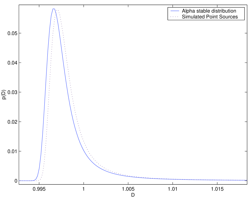
Figure 2: Comparison of the $P(D)$ distribution function of simulated point sources with an $\alpha$-stable distribution fitting the histogram data. The parameters of the EPS simulation were $\eta$=2.2 ($\alpha=1.2$), $S_{min}=10^{-3}$ (in arbitrary units), $S_{max}=10^{3}$ (in the same arbitrary units), $N_{pix}=2048\times 2048$, $N_{s}=N_{pix}$ and $FWHM=3.0$ pixels (corresponding to a true value of the normalisation $k=3.014\times 10^{-4}$ in the chosen arbitrary unit system). The normalised histogram of deflections is shown by means of a dotted line. The logarithmic moments estimators applied to that simulation give the estimates $\hat{\alpha}=1.184$ and $\hat{\gamma}=2.521\times 10^{-4}$ (corresponding to an estimated value of the normalisation $\hat{k}=3.051\times 10^{-4}$, in the chosen arbitrary unit system). Using these estimates, the corresponding $\alpha$-stable distribution with $\beta=1$ is shown using a solid line. The position of the dotted line has been slightly shifted to the right in order to make clearer the plot.

1. Sample size: there must be enough data samples to permit the non-Gaussian tail to appear and the logarithmic estimators to work. The simulations show that $\sim 10^{5}$ or more samples are more than enough to work safely. Note that a typical $512\times 512$ pixel image satisfies this condition.

2. Flux limits: in order to clearly observe the tail of the distribution, the range of fluxes of the point sources must extend over an interval big enough. In other words, there must exist a relatively few galaxies much brighter than the vast majority of low-flux ones. A dynamic range $S_{max}/S_{min}\geq 10^{4}$ suffices to guarantee the good behaviour of the tails. This condition is satisfied in CMB observations as well as in many other observations at different wavelengths.

3. Slope of the differential counts: as the distribution becomes more and more non-Gaussian, the tails grow and there are necessary more and more galaxies to ‘map’ these tails. This means that for $\alpha$ values near to $2$ it is very easy to get the shape of the distribution with few points, whereas when $\alpha$ decreases one needs a much higher number of points and a wider flux dynamic range in order to realise the tails. The results given in the two previous points are valid for $\alpha\in(1,1.5)$; for higher $\alpha$ values it is much easier to realise the tails and the $\alpha$-stable approximation holds even for smaller number of data and tighter flux cuts. On the contrary, below $\alpha=1$ the $\alpha$-stable approximation is less accurate unless the data size and the flux cuts grow accordingly.

4. Beam size, pixel size and number density of sources. The combination of the first two factors define the so-called effective resolution element of the experiment. The intuitive idea behind the effective resolution element is that, due to the smoothing produced by the instrumental beam and the finite size of the pixel, the fluctuations in the images are dumped below a certain scale that is given by the beam and pixel sizes. If the beam is sufficiently small, the effective resolution element corresponds to the pixel size, but if the beam size is bigger than the pixel size (as is usual) the effective resolution element is related to the coherence scale of the fluctuation field. For a Gaussian beam of width $\sigma_{b}$ the coherence scale is roughly equal to $\sigma_{b}$ (Rice rice (1954)), and the area $\sigma_{b}^{2}$ defines the effective resolution element. In the case of a circular Gaussian beam $\sigma_{b}$ is related the the Full Width Half Maximum (FWHM) by $FWHM=2\sigma_{b}\sqrt{2\ln{2}}$. The $\alpha$-stable approximation is shown to work optimally when there is approximately one source per effective resolution element. When the number density of sources is lower, the field is undersampled and bigger numbers of data are needed to realise the tails of the distribution. On the other hand, very faint galaxies, whose number density is much higher than one per effective resolution element, do not practically generate intensity fluctuations. In this latter case, the fluctuations are dominated by sources whose number density is just below the limit of 1 source per effective resolution element, i.e. the brightest undetected ones. Hence, the method is very sensitive to objects able to generate intensity fluctuations, that is, the source population which dominates the number counts at fluxes such that the number density is $\sim 1$ per effective resolution element or lower. Note that this limitation is not exclusive of the $\alpha$-stable model, but it is shared by every other method that works with the $P(D)$ distribution (Scheuer scheuer2 (1974)). The reason is that the level of $\sim$1 source per effective resolution element (in the sense of coherence scale explained before) roughly determines the r.m.s amplitude of the distribution whereas fainter sources only add some Gaussian noise (Franceschini et al. franceschini1 (1989), Barcons barcons (1992)). Moreover, it is not possible to distinguish between one source per effective resolution element and an infinitely large number summing up the same total flux of an individual source.

Therefore, for $\alpha\in(1,2]$ the $\alpha$-stable is a good approximation, provided that the number of data and the flux limits of the galaxies take reasonable values that are easily satisfied in usual Astronomical cases.

As an example, a $2048\times 2048$ pixel simulation was performed in which point sources were distributed following a truncated power law with flux limits $S_{min}=10^{-3}$, $S_{max}=10^{3}$ (in arbitrary units) and slope $\eta=\alpha+1=2.2$, and then ‘observed’ with a Gaussian beam of $FWHM=3.0$ pixels. The mean density of sources in the simulation was one per pixel. The resulting distribution $P(D)$ is shown in Fig. 2. The real histogram of the deflections produced by the EPS simulation (the solid line in the figure) is compared with an $\alpha$-stable distribution with the parameters extracted from the EPS simulation using the logarithmic moment estimators in eqs. (25), (26) and (27). The agreement between the two curves is very good and the relative errors in the determination of the parameters $\alpha$ and $\gamma$ (or, conversely, $\eta$ and $k$) are $\sim 1\%$ for both parameters (see figure caption).

Let us summarise the results of this section. We have proposed a set of very straightforward estimators to extract the parameters $\eta$ and $k$ which characterise the differential counts of a generic point source population. These estimators, described in equations (25) to (27), are based on the logarithmic moments of $\alpha$-stable distributions and are specifically designed to deal with non-Gaussian, asymmetric pdf s such as the one generated by point sources in the sky. From the theoretical point of view, these estimators are efficient (Kuruoğlu, 2001) whereas ‘classical’ analysis based in ordinary moments (mean, variance, skewness and so on) is not reliable since they do not converge. Moreover, the estimate of the parameters $\alpha$ and $\gamma$, directly related to the parameters $\eta$ and $k$, is direct and computationally very fast, since it only needs the calculation of two moments $L_{1}$ and $L_{2}$ (eqs. (19) and (20)). The analysis of a $2048\times 2048$ pixels takes around one second in a PC with a XEON 2.0 GHz processor. An approach based on ‘classical’ moments would require the calculation of an higher number, $N\geq 3$, of moments, their comparison with a precalculated set of values given by a certain model and, finally, finding the best parameters by means of a fit (and so on). The $\alpha$-stable assumption works well for the case of truncated EPS distributions, provided that the number of data is large enough and the ratio between the cuts $S_{max}/S_{min}$ allows the tails of the distribution to be correctly realised. By using logarithmic estimators the parameters $\eta$ and $k$ can be estimated with very small relative errors ($\sim 5\%$) for a wide range of $\eta$ values. As it happens with other existent methods on the $P(D)$ distribution, this method works optimally when the average number of sources per effective resolution element is $\sim 1$. This means that when we estimate the parameters $\eta$ and $k$ of the differential source counts we are, actually, estimating the parameters of the source population which dominates the counts in the flux interval around the $S$ value corresponding to $\sim 1$ source per effective resolution unit.

5 Point source parameter extraction from non-ideal power law number counts: realistic galaxy population models

In section 4.2 we have established the performance and the range of applicability of estimators based on the $\alpha$-stable modelling of the $P(D)$ distribution for truncated power laws, that are a fair approximation to the observed number counts. Provided that reasonable conditions of applicability of the estimators are satisfied, the results are valid for diverse fields of Astronomy, including the study of the X-ray background and the modelling of unresolved point sources at radio wavelengths.

In this section we will go one step further and consider state-of-the-art realistic number counts models. As an example, we will focus on the application of the $\alpha$-stable distributions to microwave observations and, in particular, to the images that the future ESA’s Planck mission will produce.

The study of real microwave images differ from the study of the simulations in the last section for two main reasons. First, number counts of extragalactic sources do not follow a pure power law distribution, but a more complex behaviour that depends on the emission properties of galaxies, i.e. their energy spectra, as well as their local densities and redshift evolution. The power law distribution is only a first order approximation to the real one. Second, microwave images contain not only EPS signal, but also CMB radiation, other Galactic and extragalactic foregrounds (synchrotron, free-free, dust emission and Sunyaev-Zel’dovich effect) and instrumental noise. All the above has to be taken into account in a realistic analysis. In this section we will deal with the real number count distribution of the sources. Some hints about how to deal with signal mixtures will be introduced in next section.

5.1 Extragalactic point sources at Planck frequencies

To test the efficiency of $\alpha$-stable distributions in estimating the relevant parameters, $\eta$ and $k$, of source number counts in CMB maps it is better to rely on realistic cosmological evolution models for sources. The relevant source populations at microwave frequencies are “flat”–spectrum compact radio sources, selected at cm wavelengths, and galaxies whose emission is dominated by dust, i.e. high redshift spheroids and low redshift starburst and spiral galaxies, observed in the far–IR bands. By exploiting all the available data on extragalactic sources coming from surveys at cm and far–IR wavelengths, T98 presented a phenomenological evolution model which allowed to predict source number counts in the whole frequency range around the CMB intensity peak. A thorough study on source contributions to the intensity fluctuations of the CMB was also presented in that paper. As discussed in Sect. 1, the observations of the microwave sky provided by NASA’s WMAP satellite (Bennett et al. 2003b ) and the surveys coming from VSA and CBI experiments, strongly support the predictions on number counts of EPS discussed by T98, at least up to frequencies $\nu\sim 40$ GHz. Given that “flat”–spectrum compact sources are the dominant population in this frequency range, we may confidently rely on the T98 model for simulating point sources in the sky up to $\nu\simeq 100\div 200$ GHz. On the other hand, at frequencies $\nu\geq$ 300–400 GHz many new data have been published since 1998 and most recent evolution models fit better than the T98 model the available data on source counts. These recent models (e.g., Granato et al. granato (2001), granato2 (2004)) show, in particular, a steeper slope of the differential counts of EPS at $S\sim 10-100$ mJy and for $300\leq\nu\leq 900$ GHz, where the contribution of high-redshift spheroids show up (see, e.g., Perrotta perrota (2003)). On the other hand, at fluxes $S\lesssim 0.1$ mJy all models must converge to a sub-euclidean slope in order to not exceed the integrated far-IR background. Thus, in all those flux ranges where there are no great changes of slope, the power-law approximation still holds and the $\alpha$-stable method can be effectively applied. This is the case of all (or almost) all Planck channels given the current flux limits for source detection foreseen for the mission (see Vielva et al. vielva (2003), where all the foregrounds have been taken into account). On the other hand, the method could reveal not easily appliable, or not appliable at all, to the $P(D)$ data that will come from the future surveys of the Herschel mission. In fact, current estimates on the sensitivity limits foreseen for Herschel (Negrello et al. negrello (2004)) show that, inside the flux range where the method could be able to recover the parameter $k$ and $\eta$ –i.e., for fluxes at the level of $\sim$ 1 source/beam, see Sect. 4.2–, EPS counts should show a sudden upturn, due to either the strongly positive k-correction of dust emission spectra and to the strong cosmological evolution of high-redshift star-forming spheroids.

In this first application of the method we still adopt the original T98 model since we are mostly interested in testing the method rather than using it in a specific observation scenario.

5.1.1 Radio sources

Radio loud AGNs (radio galaxies, quasars and BL-Lacs) are expected to dominate the counts in Planck LFI channels at fluxes $S\geq$1-10 mJy. At frequencies around 30 GHz the typical values for the power law slope are $\eta\sim 2.0-2.15$ (Taylor et al. taylor (2003), Mason et al. mason (2003)) at fluxes $10\leq S(\textrm{mJy})\leq 300$. At higher fluxes, the data coming from classical radio surveys at cm wavelengths show typical slope greater than the Euclidean one (i.e., $\eta>2.5$. On the other hand, at lower fluxes the power law index should keep $\sim 2.0-2.2$ down to fluxes of $S\sim$ a few $\mu Jy$ where it has to break down to lower values, for not exceeding current limits on the integrated extragalactic background (see, e.g., Haarsma & Partridge haarsma (1998), and references therein). The number of expected detections at the 30 GHz Planck channel, based on the T98 models and using the Mexican Hat Wavelet detection technique (Vielva et al. vielva (2003)), varies from $\sim 1800$ (when the emission of the rotational dust is taken into account in the simulations) to $\sim 2700$ (when it is not). Evidently, the number of detections depends on the flux detection limit attainable by the chosen technique.

5.1.2 Dusty galaxies

Both ‘normal’, i.e. spiral-like, and active galaxies show dust emission that quickly dominates over the radio emission at wavelengths shorter than a few mm. From a theoretical point of view, the physical processes that govern galaxy formation and evolution are poorly known, but there is evidence of strong cosmological evolution in the far-IR/mm region, particularly for early type galaxies (see Granato et al. granato (2001) and references therein). Therefore, it is not easy to model number counts of these source populations. SCUBA, MAMBO and IRAM surveys are rapidly providing a great amount of data in this particular energy domain and all these data are guiding the predictions on source counts and related statistics by means of phenomenological as well as physical evolution models (Toffolatti et al. T98 (1998); Guiderdoni et al. guiderdoni (1998); Granato et al. granato (2001), Rowan-Robinson rowan (2001)). Anyway, all these models predict that number counts of EPS are dominated by dusty galaxies at $\nu\geq 300$ GHz. The number of these sources detectable by Planck is variable, depending on the emission properties of the cold dust, on the cosmological evolution of sources and on the capability of detection techniques. Current estimates by Vielva et al. (vielva (2003)) based again on the T98 model with galaxies whose positions in the sky are Poisson-distributed, predict the detection of $\sim 12700$ (85 % completeness level) point sources in the 857 GHz Planck channel.

5.1.3 Total counts

Taking into account the mixture of the different types of galaxies and all the observational and theoretical constraints on them, it is evident that the number counts can not be described by a single power law as in eq. (1). Even a truncated power law as in eq. (28) is not a correct representation of the number counts. The real number counts need a slope $\eta$ that changes depending on the flux range considered. In some cases, the data can still be approximated by the sum of two or more populations whose number counts can be described by simple power laws with different slopes.

In spite of this, the $\alpha$-stable model can still be useful to extract information about the general behaviour of the dominating point source population from the analysis of the total $P(D)$. In order for this affirmation to be true, the shape of the number counts curve should be similar to a power law at least in the flux range of the dominant point sources, and the $P(D)$ should be not much different from an $\alpha$-stable . Let us see if any of these conditions are satisfied by Planck observations.

Figure 3: Predicted integral counts in the ten original Planck channels. The solid line shows the total number counts in the simulations (including both radio selected and far-IR galaxies). The dotted line is the best-fit single power law model for each channel. The fit is performed using only number counts of bright sources down to the flux at which there is approximately one source per effective resolution element, that is, the flux interval in which the statistical analysis of the $P(D)$ is sensible to the number counts law.

Figure 3 shows the $logN$–$logS$ curves for the ten Planck channels according to the T98 model. The solid lines show the total number counts in the simulations (including both radio selected and far-IR galaxies). The figure shows that the behaviour of the number counts does not correspond to a single power law. As discussed before, this is not surprising, given that the spectra and the evolution properties of sources dominating radio and far–IR source counts are quite different. However, a power law fitted to the number counts (straight dotted lines), only at fluxes greater than the one where there is approximately only one source per effective resolution element, does not depart much from the true curve. The slopes of these fits lead to best-fit slopes $\eta\sim 2.1-2.7$. The best-fit slopes and normalisations calculated for each channel are shown in table 1. According to Fig. 3, The best-fit slopes could be considered as a good approximation to the true slope of the source population which dominates the counts in the relevant flux interval (see Sect. 4.2) in each case: i.e., “flat”–spectrum radio sources in the low frequency channels, dusty galaxies in the high frequency ones.

As mentioned before, in many cases the data can be approximated by the sum of two or more populations whose number counts can be described by simple power laws with different slopes. If one of these populations happen to dominate over the others in the flux range corresponding to $\la 1$ sources per effective resolution element, the $\alpha$-stable model will be a fair approximation able to determine the parameters corresponding to such population. If there is not a dominant population, but a number $N_{p}$ of roughly equally rich populations with different slopes, the situation becomes more complex and the $\alpha$-stable model will not be correct in general. However, as $N_{p}$ increases the situation tends again to $\alpha$-stability, due to the generalised central limit theorem (Sect. 3). In this latter case, the $\alpha$-stable will allow us to determine the average parameters of the mixed source populations.

5.2 Validity of the $\alpha$-stable model

A very simple way to see if the $\alpha$-stable model is valid for the Planck point source simulations is to fit the number counts to a single power law with certain fit parameters $\alpha_{fit}$ and $k_{fit}$, then to apply the logarithmic estimators in eqs. (25), (26) and (27) to realistic Planck EPS simulations in order to obtain some estimated $\alpha_{logm}$ and $k_{logm}$, and then check the agreement between the two sets of values.

Table 1: Comparison between the point source parameters $\alpha$ and $k$ extracted using logarithmic estimators (denoted by the ‘logm’ subscript) and the best-fit power law (denoted by the ‘fit’ subscript) for the nine frequencies of the T98 Planck EPS simulations. The normalisation $k$ is expressed in units of Jy^α pixel^-2. A good agreement between the fit and the logm values indicates that the $\alpha$-stable approximation is valid as a means for estimating the slope and the normalisation of the differential number counts of the dominating point source population. Relative errors are calculated as $r_{x}=100\times\left|x_{logm}-x_{fit}\right|/x_{fit}$, $x$ representing either $\alpha$ or $k$.

$\nu$ (GHz)	$\alpha_{fit}$	$\alpha_{logm}$	$r_{\alpha}$	$k_{fit}$	$k_{logm}$	$r_{k}$
30	1.22	1.24	2	6.63$\times 10^{-4}$	5.81$\times 10^{-4}$	12
44	1.18	1.18	0	1.77$\times 10^{-4}$	1.73$\times 10^{-4}$	2
70	1.16	1.13	3	4.36$\times 10^{-5}$	4.72$\times 10^{-5}$	8
100	1.18	1.15	3	4.20$\times 10^{-5}$	4.30$\times 10^{-5}$	3
143	1.30	1.37	5	2.67$\times 10^{-5}$	1.64$\times 10^{-5}$	39
217	1.58	1.67	6	4.59$\times 10^{-6}$	2.22$\times 10^{-6}$	52
353	1.83	1.77	3	10.54$\times 10^{-5}$	8.81$\times 10^{-6}$	16
545	1.83	1.76	4	8.19$\times 10^{-5}$	6.61$\times 10^{-5}$	19
857	1.75	1.69	3	6.44$\times 10^{-4}$	5.50$\times 10^{-4}$	15

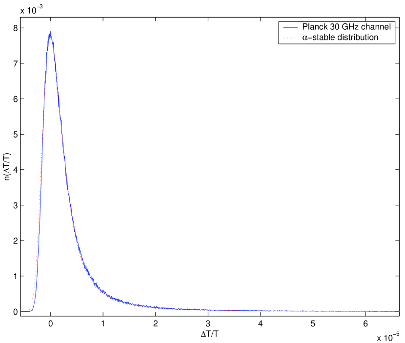
Figure 4: Comparison of the histogram of the distribution of deflections due to extragalactic point sources in the 30 GHz Planck channel (solid line) and an $\alpha$-stable distribution (dotted line). The $\alpha$-stable distribution has the $\alpha$ and $\gamma$ parameters that were estimated by means of logarithmic estimators on the EPS data: $\hat{\alpha}=1.24$ and $\hat{\gamma}=7.02\times 10^{-8}$. The EPS map is expressed in $\Delta T/T$ units.

We performed realistic point source simulations using the T98 model. The simulated sky maps were filtered using the beam sizes (circular Gaussian approximation) and the pixel scales of the 9 Planck channels. The number counts of the T98 model were fitted to a straight line in order to obtain the values of the parameters $\alpha_{fit}$ and $k_{fit}$ that better fit the model in the flux range of interest. Taking into account the results of section 4.2, the fit was performed using the number counts at fluxes $S>S_{1}$, where $S_{1}$ is flux over which there is approximately one source per effective resolution element. The parameters $\alpha$ and $k$ were then estimated for each channel using logarithmic moments estimators. The results can be seen in table 1. Table 1 shows that the validity of the $\alpha$-stable model is better for some channels than for others. The relative errors in the parameter $\alpha$ are only a few percent. The agreement in $k$ is worse because equations (15) and (27) are very sensitive to the estimated value of $\alpha$ and therefore relatively small errors in $\alpha$ can lead to big errors in $k$. For the case of the 30 GHz channel $k_{fit}$ and $k_{logm}$ agree up to a $12\%$, and the agreement in the 44, 70 and 100 GHz is even better, whereas for the worst case (217 GHz) the difference between the two values rises to a $52\%$. For the 857 GHz channel the relative difference between $k_{fit}$ and $k_{logm}$ is $15\%$. Therefore, we can conclude that the $\alpha$-stable is a good model for the T98 sources, and that the logarithmic moments estimators can recover quite well the most representative value of $\alpha$ for the fluxes greater than the flux over which there is approximately one source per effective resolution element. This value varies depending on the channel, and corresponds in general to a few tens of mJy in the Planck case. The estimation of $k$ is less reliable in general, but the method can be still useful, however, as a means to constrain its value.

The results of Table 1 show that the agreement between the fitted $\alpha$ and the value estimated with the logarithmic moments is worse for the case of the intermediate channels. This result is easily explained taking into account the previous discussion about the physical nature of the galaxies at microwave frequencies. Whereas the low-frequency channels of Planck (30, 44 an 70 GHz) are dominated by radio-selected point sources and the high-frequency ones (545 and 857) are mainly populated by far-IR galaxies, at the intermediate frequencies the mixing of two main different populations distorts the shape of the $P(D)$ distribution, making the $\alpha$-stable approximation less valid. As an example of this, in Figs. 4 and 5 the histogram of the deflection distribution due to the EPS as two of the Planck channels are compared with the $\alpha$-stable distributions generated using the corresponding estimated $\alpha_{logm}$ and $k_{logm}$. Figure 4 corresponds with the 30 GHz channel whereas Fig. 5 corresponds with the 217 GHz case. For this latter channel, the basic shape of the $P(D)$ is very well approximated by the $\alpha$-stable, but small differences in the region of the tail, barely visible to the eye, are enough to hamper the validity of the $\alpha$-stable model. On the contrary, for the 30 GHz case in Fig. 4 the agreement between the two curves is good along all the curve, and specially good in the tail, where the most important information is stored, leading to a good estimation of the slope $\alpha$ and the normalisation $k$ of the radio source counts.

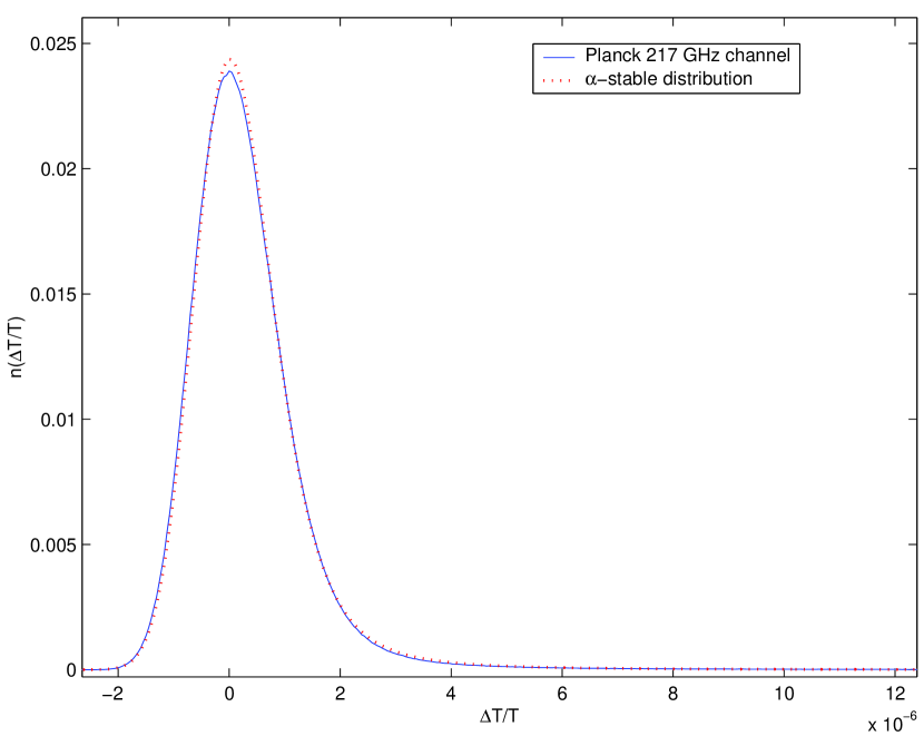
Figure 5: Comparison of the histogram of the distribution of deflections due to extragalactic point sources in the 217 GHz Planck channel (solid line) and an $\alpha$-stable distribution (dotted line). The $\alpha$-stable distribution has the $\alpha$ and $\gamma$ parameters that were estimated by means of logarithmic estimators on the EPS data: $\hat{\alpha}=1.67$ and $\hat{\gamma}=0.34\times 10^{-10}$. The EPS map is expressed in $\Delta T/T$ units.

6 Point source parameter extraction in presence of noise and other signals

We have shown that the tools based on $\alpha$-stable analysis are applicable to astronomical data such as those that will be observed by the low and high frequency channels of Planck. Even when the mixture of two roughly equally dominant different populations makes impractical to determine the normalisation $k$ of the mixture, it is still possible to set constraints to the global slope of the number counts. But the previous discussion was restricted only to the emission of point sources. Apart form the EPS population, the microwave sky contains emissions from many other astronomical sources (‘foregrounds’), CMB radiation and instrumental noise. Therefore, it is not possible in general to observe the point sources independently from the other components. Though the addition of these other signals does not modify the $\alpha$-stable nature of the point sources $P(D)$, it affects the way we can learn the parameters $\alpha$ and $\gamma$ from the data. The estimate of these parameters can get very complicated in presence of all these components. In the following we will consider the simplified (albeit very commonly found in practise) problem of a mixture of a Gaussian random process and EPS. This is the case when instrumental noise (generally modelled as Gaussian white noise) is added to the EPS signal by the detector. In the case of CMB observations, that would be the case as well in ‘clean’ sky areas (that is, not affected by foreground contamination). We shall comment about this in the next section.

6.1 Parameter estimation in Gaussian and $\alpha$-stable mixtures

Let us consider the case of a mixture of EPS ‘confusion noise’ and a Gaussian signal. This Gaussian signal can be instrumental noise or even the CMB itself if is has not been previously separated from the data. The Gaussian distribution is a particular case of the $\alpha$-stable family with $\alpha=2$. The mixture of two $\alpha$-stable distribution with different $\alpha$ index is not an $\alpha$-stable distribution. Therefore, the simple logarithmic moments estimators presented in Sect. 4 are not valid.

The characteristic function of the mixture of two independent random variables can be expressed as the product of the characteristic functions of the two original variables. That means that the characteristic function of a mixture of an $\alpha$-stable distribution $S_{\alpha}(\beta,\gamma,\mu)$ and a Gaussian $\mathcal{N}(\mathit{0},\sigma)$ is

$$\psi_{mix}(w)=\exp\left\{i\mu w-\gamma\left|w\right|^{\alpha}B_{w,\alpha}+\frac{1}{2}\sigma^{2}w^{2}\right\},$$ (29)

where $B_{w,\alpha}$ is defined in eq. (13). Applying centro-symmetrisation as in eq. (18) we have

$$\psi^{S}_{mix}(w)=\exp\left[-2\gamma\left|w\right|^{\alpha}-\sigma^{2}w^{2}\right].$$ (30)

The parameter extraction in the case of mixtures with characteristic functions such as in eq. (30) is a very difficult problem that has not been totally solved yet. It has been studied by Ilow & Hatzinakos (ilow (1998)), who presented some basic ideas based on the empirical characteristic function (ecf)

$$\hat{\psi}_{N}(w)\equiv\frac{1}{N}\sum_{m=1}^{N}e^{iwx(m)}.$$ (31)

The ecf is a complex random variable and its expected value coincides with the true characteristic function of the distribution when the $x(m)$ samples are i.i.d. Ilow & Hatzinakos (ilow (1998)) described two types of methods based on the ecf to perform the estimate of the parameters $\alpha$, $\gamma$ and $\sigma$ in eq. (30): minimum distance methods and moment-type methods. We tested both kind of methods and found that the moment-type ones suffer from problems of stability in the particular case under study. Therefore, we will focus on the minimum distance method.

6.1.1 Minimum distance method

In the minimum distance method, the estimate of the parameters $\Theta=(\alpha,\gamma,\sigma)$ is obtained in the optimisation process

$$\min_{\Theta}\int_{-\infty}^{\infty}\left|\hat{\psi}_{N}(w)-\psi_{\Theta}(w)\right|^{2}W(w)dw,$$ (32)

where $W(w)$ is an appropriate weighting function. For example, the choice $W(w)=\exp(-w^{2})$ allows the integral (32) to be solved by means of Gauss-Hermite quadratures, which is computationally convenient. Thus, the estimate of the parameters $\Theta$ is reduced to a minimisation over three parameters. An interesting possibility appears when one of the parameters, generally $\sigma$, is a priori known. Then the minimisation gets much more simple.

The minimum distance method is as far as we know the best choice present at this moment in the literature, but it may present some problems. In particular, the choice of the weighting function $W(w)$ is arbitrary. The choice $W(w)=\exp(-w^{2})$ is useful from the computational point of view but it may mask important features of the ecf. We are currently working in the elaboration of more robust methods, that will be the scope of future works. For the moment, let us restrict the discussion to the minimum distance method.

6.2 Some simple tests

In order to test the minimum distance method we performed a set of simulations of point sources whose number counts follow a truncated power law, adding a Gaussian white noise to the beam-convolved sources. The size of the simulations was $N_{pix}=1024\times 1024$ and the cuts of the truncated power law were set so that $S_{max}/S_{min}=10^{6}$ in arbitrary units. The beam was set to FWHM = 3 pixels. For the sake of clarity, the simulations contains one source on average per pixel, that corresponds with $\gtrapprox 1$ source per effective resolution element (as defined in section 4.2), given the value of the FWHM chosen.

We have tested the performance of the method as a function of the relative contribution of each component of the mixture. In order to do that, the slope of the EPS law was set to $\eta=2.2$ ($\alpha=1.2$). Fifty simulations were performed for each case. We fixed the contribution of the Gaussian noise to $\sigma_{G}=1$ (in arbitrary units) and let vary the value of the minimum source flux $S_{min}$. This has the effect of varying the rms of the EPS contribution, i.e. the $\gamma_{S}$ of the $\alpha$-stable distribution. In other words, we fix the second term in the exponential of equation 30 and vary the first one. As described in section 3, we write the scale parameter of the Gaussian contribution to the characteristic function as $\gamma_{G}=\sigma_{G}^{2}/2$ (where $\sigma_{G}$ is the Gaussian noise dispersion). Then we can study the performance of the method as the ratio $\gamma_{S}/\gamma_{G}$ varies. Results are shown in Fig. 6.

The method obtains its better performance when the contributions of the $\alpha$-stable distribution and the Gaussian noise are comparable in the characteristic function. Inside the interval $-1\leq\log(\gamma_{S}/\gamma_{G})\leq 1$ the relative errors in the determination of the three parameters are of a few percent. When the Gaussian contribution dominates ($\log(\gamma_{S}/\gamma_{G})<-1$) the estimator ‘sees’ only a Gaussian contribution and tries to adjust it to the three parameters by considering that the two terms inside the exponential in eq. (30) are identical Gaussian exponents. Therefore, it wrongly gives $\alpha$ a value of 2, underestimates the true $\gamma_{G}$ by a factor $\sim 50\%$ and greatly overestimates $\gamma_{S}$.

When the point source population overdominates the method tends to assign the central parts of the distribution to an almost inexistent Gaussian and to fit the remaining tail to an $\alpha$-stable that is more impulsive than the real one, producing lower values of $\alpha$ than the true ones. The $\gamma_{S}$ parameter is well established in this region, but the estimated $\gamma_{G}$ gets artificially high.

Figure 6: Performance of the minimum distance method as a function of the relative contribution of the mixture components. The top panel shows the relative error in the determination of the Gaussian dispersion $\sigma_{G}$. The relative error in the determination of the $\alpha$-stable parameter $\gamma$ is shown in the middle panel. The bottom panel shows the relative error in the determination of the index $\alpha$. Statistical error bars are shown in each case.

In many real cases, the level of the Gaussian contribution is a priori known. For example, the noise level of an instrument is generally well known in most experiments. If that is the case, the minimisation (32) can be simplified by fixing the value of $\sigma$ (that is, $\gamma_{G}$). Then the minimisation is performed in the two-dimensional parameter space $(\alpha,\gamma)$. In this case, the estimates of the $\alpha$-stable parameters improve significantly in the low $\gamma_{S}/\gamma_{G}$ regime. As an example, in the previous test experiment for $\gamma_{S}=7.48\times 10^{-3}$ (corresponding to the point $\log(\gamma_{S}/\gamma_{G})=-1.82$ in figure 6), the estimates of the parameters when $\sigma$ was unknown are $\hat{\alpha}=1.75\pm 0.22$, $\hat{\gamma_{S}}=0.09\pm 0.11$, whereas if the value of $\sigma$ is fixed the parameters are much better estimated, $\hat{\alpha}=1.2\pm 0.1$, $\hat{\gamma_{S}}=7.54\times 10^{-3}\pm 0.91\times 10^{-3}$. Our tests show that if $\sigma$ is well known it is safe to apply the method until ratios $\log(\gamma_{S}/\gamma_{G})\simeq-2.2$, with few percent relative errors in $\alpha$ and $\gamma$. Below that threshold, the performance drops quickly.

In the intermediate $\gamma_{S}/\gamma_{G}$ regime the improvement is not so spectacular: as an example, for $\gamma_{S}=0.472$ (corresponding to the point $\log(\gamma_{S}/\gamma_{G})=-0.025$ in figure 6), the results were $\hat{\alpha}=1.2\pm 0.02$, $\hat{\gamma_{S}}=0.476\pm 0.02$ when $\sigma$ was unknown and $\hat{\alpha}=1.2\pm 0.01$, $\hat{\gamma_{S}}=0.466\pm 0.006$ when it was known.

In the high $\gamma_{S}/\gamma_{G}$ regime the knowledge of $\sigma$ gives few information and the results are practically the same when it is known than when it is not. Of course, if the EPS largely dominate the mixing it may be a better idea just to forget about the minimum distance method and to apply directly the logarithmic moment estimators of section 4, as the data can be regarded as an $\alpha$-stable contaminated with a small amount of noise. To test this idea we just applied the logarithmic moment estimators to our simulations. The results show that if $\log(\gamma_{S}/\gamma_{G})\lesssim 0.6$ the logarithmic moments fail, as expected, but over that threshold they work very well. As an example, for $\gamma_{S}=7.5$ (corresponding to $\log(\gamma_{S}/\gamma_{G})=0.57$) the minimum distance method obtained $\hat{\alpha}=1.27\pm 0.47$, $\hat{\gamma_{S}}=6.48\pm 3.46$, whereas direct application of the logarithmic moments gives $\hat{\alpha}=1.19\pm 0.01$, $\hat{\gamma_{S}}=7.24\pm 0.12$. At higher $\gamma_{S}/\gamma_{G}$ ratios the validity of the logarithmic moment estimators is even more justified: for $\gamma_{S}=118.6$ (corresponding to $\log(\gamma_{S}/\gamma_{G})=2.37$) the minimum distance method obtained $\hat{\alpha}=0.55\pm 0.80$, $\hat{\gamma_{S}}=22.0\pm 22.6$, whereas direct application of the logarithmic moments gives $\hat{\alpha}=1.19\pm 0.01$, $\hat{\gamma_{S}}=109\pm 4$. A small negative bias ($\sim-5\%$) seems to appear in the determination of $\gamma_{S}$ for high $\gamma_{S}/\gamma_{G}$ ratios, probably due to the presence of the Gaussian interference.

Taking all the previously said into account, the reccomendation is to use the minimum distance method when the expected $\log(\gamma_{S}/\gamma_{G})\leq 1$ and just the logartihmic moments estimator for higher $\alpha$-stable / Gaussian ratios. Fixing the value of the Gaussian contribution with a priori information allows us to determine the $\alpha$-stable parameters safely up to $\log(\gamma_{S}/\gamma_{G})\sim-2$, whereas if $\sigma$ has to be determined the safety region finishes around $\log(\gamma_{S}/\gamma_{G})\sim-1$.

We also performed simulations varying the slope $\eta$ ($\alpha$) at a given $\gamma_{S}/\gamma_{G}$ (both contributions were set so that the contribution to the characteristic function of both components are the same). The estimates for the three parameters $\alpha$, $\gamma$ and $\sigma$ have low relative errors ($\sim 10\%$) around the values $\alpha\sim 1.0-1.6$. Far from this region, the estimates become worse, specially in the low-$\alpha$ regime, where bigger simulations or larger dynamic ranges (the ratio $S_{max}/S_{min}$) are needed in order to ‘map’ the $\alpha$-stable tail correctly. On the other hand, when $\alpha$ gets too close to 2 the two distributions are almost Gaussian and is very hard to distinguish them.

7 Some considerations about EPS parameter estimation at Planck frequencies

As mentioned before, the microwave sky as observed by any of the many experiments that are now being carried out or in preparation is a mixture of CMB, galactic foregrounds, EPS, galaxy clusters and instrumental noise and systematics. The full study of the EPS’ confusion noise in such a complicated mixture is out of the scope of this work and will be addressed in future studies. However, some considerations about the expected problematics and possible results for the future Planck mission can be hinted in base on the results of previous sections.

Galactic foregrounds will be a major problem for the application of the techniques presented in this work. Foreground signature is nor Gaussian nor $\alpha$-stable, and therefore neither the logarithmic moment estimators nor the minimum distance method for Gaussian plus $\alpha$-stable mixtures are expected to work well under strong Galactic contamination circumstances. Neither will do any other of the existent methods for the $P(D)$ study.

On the other hand, in areas of the sky where the Galactic contamination is low there would be present basically EPS, CMB and instrumental noise (as well as some secondary CMB anisotropies due to SZ effect). CMB is Gaussian or near-Gaussian distributed, and therefore in such sky areas the minimum distance method presented in section 6.1.1 can be applied, just considering the mixture of CMB plus noise as a single Gaussian component with joint effective variance $\sigma_{eff}^{2}=\sigma_{CMB}^{2}+\sigma_{n}^{2}$. Such approach should success for the channels where the EPS signal is more relevant, that is, the low frequency channels (30 and 44 GHz) where radio sources are dominant and the high frequency channels (545 and 857 GHz) where dusty galaxies are dominant.

Unfortunately, precisely at those channels the foreground contribution is expected to be very high. In particular, at 857 GHz will be practically impossible to find a single patch of the sky where the Galactic dust emission is subdominant with respect to CMB. Foreground-free areas of the sky could be found outside the Galactic plane in the intermediate Planck channels, where EPS are expected to be so faint that they will be under the detection threshold of the minimum distance method.

A more interesting possibility appears if the foreground emission can be somehow removed from the data before the analysis. As mentioned in the Introduction, there are several different statistical component separation methods that are able, given some amount of a priori knowledge about the statistical properties of the different components, to extract them. These methods in general are not able to deal with unresolved point sources, and normally a residual map containing noise, EPS and some leftovers of the components that have not been perfectly separated is obtained as a by-product of the separation. Note that most component separation assume that the non-separable noise is Gaussian, which is not true in presence of EPS. This may introduce errors in the separation of the foregrounds. An interesting possibility that will be studied in the future is to introduce our knowledge on the $\alpha$-stable nature of EPS confusion noise in the component separation method.

If a perfect separation was possible, the residual map would contain just instrumental noise and EPS. In that ideal case and for the T98 EPS model and the noise levels expected for Planck, the ratios between the point source and the Gaussian noise contributions to the residual map would be $\log(\gamma_{S}/\gamma_{G})=2.77,\ 3.09,\ 3.31,\ 2.05,\ 0.75,\ 0.30,\ 0.17$ and -0.12 for the 30, 44, 70, 100, 143, 217, 353, 545 and 857 GHz channels, respectively. According with the results in section 6, such ratios should allow the methods presented in this work to obtain the $\alpha$-stable parameters of the $P(D)$ with small errors for all the channels.

The real case will not be so optimistic as the one just mentioned, but not so pessimistic as the case in which all the foregrounds are fully present. The study of the performance of the $\alpha$-stable methods after the application of a component separation method –such as the Maximum Entropy method (Hobson et al. hobson (1999)), for example– will be carried out in a future work.

8 Conclusions

In this work we introduce the formalism of $\alpha$-stable distributions as a useful tool for the modelling and the statistical study of number counts of undetected point sources in astronomical images. When the number of faint point sources in an image is large, the unresolved EPS contribution creates a ‘confusion noise’ that can be studied to obtain information about the parent EPS population.

We have shown that when the differential number counts of point sources follow a simple power law the characteristic function of the resultant distribution of intensity (or temperature) fluctuations is exactly an $\alpha$-stable one. In Sect. 3 we briefly review the many definitions and properties concerning the $\alpha$-stable formalism. The $\alpha$-stable model allows us to model non-Gaussian, impulsive distributions in a flexible way and with a reduced number of parameters. The mathematical foundation of $\alpha$-stable analysis is well established and useful results such as the generalised central limit theorem are available. The $\alpha$-stable distributions include the Gaussian distribution as a particular case.

We have shown as well that, under reasonable conditions, the $\alpha$-stable model is well suited to describe point source populations following truncated power law number counts. We also have shown that even if the number distribution in flux is not a pure power law the $\alpha$-stable model may be useful to estimate the parameters of the dominant source population. In particular, the $\alpha$-stable model has been proved to be useful and very efficient in recovering the $k$ and $\eta$ parameters of the EPS number counts foreseen for the highest and the lowest frequency channels of the Planck surveyor mission, where point sources give the dominant contribution to CMB fluctuations. As the EPS number counts in these channels are strongly dominated by flat-spectrum radio sources (at low frequencies, LFI channels) and by dusty galaxies (at high frequencies, HFI channels), the method discussed here has proved helpful in determining the main parameters of the differential number counts of both populations.

The $\alpha$-stable model allows us to design efficient and computationally fast estimators to extract the physical parameters of the EPS populations from $P(D)$ distribution. In particular, the logarithmic moments estimators are able to determine the slope $\eta$ and the normalisation $k$ of the EPS population with relative errors of a few percent over a wide range of conditions. The method is shown to work optimally in the case in which there is approximately one source per effective resolution element.

Even when the EPS signal is mixed with Gaussian interference, it is possible to estimate its parameters using the empirical characteristic function, given by eq. (31). We suggest a minimum distance method that is able to deal with the presence of Gaussian noise in a wide range of values of the ratio $\gamma_{S}/\gamma_{G}$.

Furthermore, the method uses all the information content of the data, taking into account bright sources as well as very faint ones which contribute to the confusion noise distribution. Anyway, as discussed in section 4.2, the $\alpha$-stable model works optimally in the case of approximately one source per effective resolution element and, thus, its maximum efficiency is reached at fluxes corresponding to this source density. An interesting possibility is to complement the information extracted with this technique with other methods. For example, by detecting and counting bright sources it is possible to obtain the slope $\eta$ and the normalisation $k$ in the high flux range. These quantities can be compared with the ones obtained by this method for studying the differences among source populations which dominate the counts at high and intermediate fluxes. The way to proceed should be detecting first the bright resolved sources and, once removed these sources from the data –for example masking the area occupied by them–, analysing the $P(D)$ of the unresolved sources by means of the statistical estimators introduced in this work. The statistical study of the $P(D)$ allows us to go below the detection threshold. The flux limit these methods can reach depend strongly on the characteristic of the experiment: in absence of noise and other foregrounds, the theoretical limit is the flux corresponding to approximately one source per effective resolution element. In presence of noise and foregrounds, this limit will be higher and must be determined for each particular case.

As mentioned before, the $\alpha$-stable model works well even there is the presence of two or more source populations with different slopes of the number counts, provided that the departure from a simple power-law is not extreme in the relevant flux range. Then, techniques such as the logarithmic moments estimators are able to estimate a single slope that corresponds to the one of the dominant source population. It is possible, however, to refine the results. A method similar to the minimum distance method presented in Sect. 6.1.1 can be conveniently modified to include more than one different $\alpha$-stable components in order to determine the parameters $k$ and $\eta$ of two or, possibly, more source populations.

Work to obtain an optimal technique to deal with $\alpha$-stable mixtures is currently in progress.

In this work we considered that the spatial distribution of the sources in the sky is uniform. However, the sources are expected to show some degree of autocorrelation. Source clustering will produce a broadening in the $P(D)$ distribution (Barcons barcons (1992)). This effect should be taken into account in a future work. We did not take into account the presence of Sunyaev-Zel’dovich (SZ) effect in the CMB maps. The signature of SZ clusters is expected to be similar in nature to the signature of EPS and, thus, the formalism of this work could be applied to it. At frequencies $\nu<217$ GHz the SZ effect will have a negative contribution to the maps, producing skewed $P(D)$ distributions with negative tails. Several ways of discriminating between unresolved point sources and SZ clusters in CMB maps have been studied by Rubiño-Martín & Sunyaev (rubi (2003)).

The previous conclusions can be applied to different fields in Astronomy including the X-ray background, radio Astronomy and, in general, to all the observations in which it is interesting the study of the statistical properties of undetected point sources.

The potentialities of the $\alpha$-stable modelling go further than the designing of estimators such as the ones presented in this work. The $\alpha$-stable model allows us to use techniques present in the signal processing literature for achieving a complete probabilistic description of the data that can be used for more ambitious goals such as Bayesian estimation, denoising, etc. Future works will explore these interesting possibilities.

- (1) Abramowitz, M. & Stegun, A., ‘Handbook of mathematical functions’, Dover Publications, 1971.
- (2) Argüeso, F., González-Nuevo, J. & Toffolatti, L., 2003, ApJ, 598, 86.
- (3) Barcons, X., 1992, ApJ, 396, 460.
- (4) Bennett, C.L., Halpern, M., Hinsaw, G. et al. 2003a, ApJS, 148, 1.
- (5) Bennett, C.L., Hill, R.S., Hinsaw, G. et al. 2003b, ApJS, 148, 97.
- (6) Condon, J.J., 1974, ApJ, 188, 279.
- (7) Condon, J.J. & Dressel, L.L., 1978, ApJ, 222, 745.
- (8) De Zotti, G., Franceschini, A., Toffolatti, L., Mazzei, P., & Danese, L., 1996, Astrophys. Lett. & Comm., Vol. 35, 239.
- (9) De Zotti, G., Toffolatti, L., Argüeso, F., Davies, R.D., Mazzotta, P., Partridge, R.B., Smoot G.F. & Vittorio, N., 1999, 3K cosmology, Proceedings of the EC-TMR Conference held in Rome, Italy, October, 1998. Woodbury, N.Y. : American Institute of Physics, vol. 476, 204.
- (10) Feller, W, ‘An Introduction to Probability Theory and its Applications’, Vol II, Wiley & Sons, 1966.
- (11) Franceschini, A., Toffolatti, L., Danese, L. & de Zotti, G., 1989, ApJ, 344, 35.
- (12) Granato, G.L., Silva, L., Monaco, P., Panuzzo, P., Salucci, P., de Zotti, G. & Danese, L., 2001, MNRAS, 324, 757.
- (13) Granato, G.l., de Zotti, G., Silva, L., Bressan, A. & Danese, L., 2004, ApJ, 600, 580.
- (14) Guiderdoni, B., Hivon, E., Bouchet, F.R. & Maffei, B., 1998, MNRAS, 295, 877.
- (15) Haarsma, D.B. & Partridge, R.B., 1998, ApJ, 503, 5.
- (16) Hewish, A. 1961, MNRAS, 123, 167.
- (17) Hobson, M.P., Barreiro, R.B., Toffolatti, L., Lassenby, A.N., Sanz, J.L., Jones, A. & Bouchet, F., 1999, MNRAS, 306, 232.
- (18) Hu, W. & Dodelson, S., 2002, ARA&A, 40, 171.
- (19) Ilow, J. & Hatzinakos, D., 1998, Signal Processing, 65, 199.
- (20) Komatsu, E., Kogut, A., Nolta, M.R. et al., 2003, ApJS, 148, 119.
- (21) Kuruoğlu, E.E., 1998, ‘Signal processing in -stable noise environments: a least -norm approach’, PhD thesis, University of Cambridge.
- (22) Kuruoğlu, E.E., 2001, IEEE Trans. Signal Proc., 49, 2192.
- (23) Lévy, P., 1925, ‘Calcul des probabilités’, Paris, Gauthier-Villars.
- (24) Mandolesi, N. Lawrence, C.R., Bersanelli, M. et al. 1998, proposal submitted to ESA for the Planck Low Frequency Instrument.
- (25) Mason, B.S., Pearson, T.J., Readhead, A.C.S. et al. 2003, ApJ, 591, 540.
- (26) Middleton, D., 1977, IEEE Transactions on Electromagnetic Compatibility, Vol EMC-19, 3, 106.
- (27) Negrello, M., Magliocchetti, M., Moscardini, L., De Zotti, G., Granato, G.L. & Silva, L., 2004, MNRASsubmitted, astro-ph/0401199.
- (28) Nikias, C.L. & Shao, M., ‘Signal Processing with -Stable Distributions and Applications’, Wiley & Sons, 1995.
- (29) Perrotta, F., Magliocchetti, M., Baccigalupi, C., Bartelmann, M., De Zotti, G., Granato, G.L., Silva, L. & Danese, L., 2003, MNRAS, 338, 623.
- (30) Pierpaoli, E., 2003, ApJ, 589, 58.
- (31) Puget, J.L. Efstathiou, G., Lamarre, J.M. et al. 1998, proposal submitted to ESA for the Planck High Frequency Instrument.
- (32) Rice, S.O., 1954, Selected papers on Noise and Stochastic Processes’, ed. N. Wax, Dover Publ. Inc. (N. Y.).
- (33) Rowan-Robinson, M., 2001, ApJ, 549, 745.
- (34) Rubiño-Martín, J.A. & Sunyaev, R.A., 2003, MNRAS, 344, 1155.
- (35) Samorodnitsky, G. & Taqqu, M.S., ‘Stable non-Gaussian random processes: stochastic models with infinite variance’, New York, NY: Chapman & Hall, 1994.
- (36) Scheuer, P.A.G., 1957, Proc. Camb. Phil. Soc., 53, 764.
- (37) Scheuer, P.A.G., 1974, MNRAS, 166, 329.
- (38) Shao, M. & Nikias, C.L., 1993, Proc. of IEEE, 81, 986.
- (39) Taylor, A.C. et al. 2003, MNRAS, 341, 1066.
- (40) Toffolatti, L., Argüeso, F., De Zotti, G., Mazzei, P., Franceschini, A., Danese, L. and Burigana, C. 1998, MNRAS, 297, 117.
- (41) Vielva, P., Martínez-González, E., Gallegos, J., Toffolatti, L. & Sanz, J. L., 2003, MNRAS, 344, 89.