Three years in the coronal life of AB Dor

The young active star AB Dor (K1 IV-V) has been observed 16 times in the last three years with the XMM-Newton and Chandra observatories, totalling 650 ks of high-resolution X-ray spectra. The XMM/RGS observations with the highest and lowest average emission levels have been selected to study the coronal properties of AB Dor in two different activity levels. We compare the results based on the XMM data with those obtained from a higher resolution Chandra/HETG spectrum, using the same line-based analysis technique. We have reconstructed the plasma Emission Measure Distribution vs. temperature (EMD) in the range log $T$(K)$\sim$6.1–7.6, and we have determined the coronal abundances of AB Dor, obtaining consistent results between the two instruments. The overall shape of the EMD is also consistent with the one previously inferred from EUVE data. The EMD shows a steep increase up to the peak at log $T$(K)$\sim$6.9 and a substantial amount of plasma in the range log $T$(K)$\sim$6.9–7.3. The coronal abundances show a clear trend of increasing depletion with respect to solar photospheric values, for elements with increasing First Ionization Potential (FIP), down to the Fe value ([Fe/H] = –0.57), followed by a more gradual recovery of the photospheric values for elements with higher FIP. He-like triplets and Fe xxi and Fe xxii lines ratios indicate electron densities log $n_{\rm e}\sim 10.8$ cm^-3 at log $T$(K)$\sim 6.3$ and log $n_{\rm e}\sim 12.5$ cm^-3 at log $T$(K)$\sim$7, implying plasma pressures steeply increasing with temperature. These results are interpreted in the framework of a corona composed of different families of magnetic loop structures, shorter than the stellar radius and in isobaric conditions, having pressures increasing with the maximum plasma temperature, and which occupy a small fraction ($f\sim 10^{-4}$–$10^{-6}$) of the stellar surface.

1 Introduction

AB Dor (HD 36705, K1 IV-V) is a frequent target for studies on stellar activity. Almost arrived in the main sequence, with an age of $\sim$20–30 Myr (Collier Cameron & Foing, 1997), it has a high rotation rate ($P_{\rm rot}$=0.5148 d), and persistent large-scale magnetic field patterns in its photosphere (see Donati et al., 1999; Hussain et al., 2002, and references therein). Two companions, not expected to interact with AB Dor, have been detected in the vicinity. The dM4e star Rossiter 137B (AB Dor B), detected as a faint source also in X-rays (Vilhu & Linsky, 1987), is 10$\arcsec$ away from the main source, while the third companion is a very low-mass star (0.08–0.11 M_☉) at a distance of 0.2$\arcsec$–0.7$\arcsec$ (3–10 a.u.) from the primary (Guirado et al., 1997). The contribution of the companions to the X-ray spectrum of the main source can be considered negligible, essentially because the quiescent X-ray emission of the companions scales as their bolometric luminosity (in fact, for their young age, all the stars in the system emit close to the saturation level of $L_{\rm X}$/$L_{\rm bol}\sim$10^-3). AB Dor has been observed with the main space observatories in the UV, EUV, and X-rays, like HST, FUSE, ROSAT, BeppoSAX, ASCA and EUVE (see Vilhu et al., 1998; Ake et al., 2000; Schmitt et al., 1998; Kuerster et al., 1997; Maggio et al., 2000; Rucinski et al., 1995; Mewe et al., 1996; Sanz-Forcada et al., 2002, and references therein), showing rotational modulation in some lines formed in the transition region, and a corona dominated by material at temperatures of log $T$(K)$\sim$6.7–7.3, significantly higher than in the solar quiescent corona. Most recently, initial results from the first XMM observations of AB Dor, taken in May and June 2000, have been presented by Güdel et al. (2001), while a preliminary analysis of the first Chandra observation was made by Linsky et al. (2001).

Figure 1: X-ray light curves from the observations analyzed in this work: ($a$) and ($b$): XMM/EPIC-pn light curves of rev. #091 and #205; ($c$): Chandra/HETG 1st order light curve of AB Dor A. The lower axis indicates time in days, and the upper axis reports the rotational phase, using ephemeris by Innis et al. (1988). Variations of 35–50% in the flux level are found during each of the three observations.

Rotational modulation up to a factor $\sim 2$ has been detected in C iii and O vi lines which form in the upper chromosphere and in the transition region (Ake et al. 2000), but only at about the 15% level for the X-ray emission observed with ROSAT (Kürster et al. 1997). Several EUV and X-ray spectroscopic studies show that the corona of AB Dor is dominated by plasma at temperatures of log $T$(K)$\sim$6.7–7.3, significantly higher than in the solar quiescent corona. On the other hand, only few determinations of the plasma density have been published up to date: using density-sensitive C iii lines in orpheus and fuse spectra, densities of $\sim 10^{11}$ cm^-3 or more at $T\sim 80000$ K have been determined by Schmitt et al. (1998) and by Ake et al. (2000), while Güdel et al. (2001) have estimated a coronal density of $3\times 10^{10}$ cm^-3 at $T\sim 2\times 10^{6}$ K using the He-like O vii emission line triplet; finally, densities of the order of $10^{12}$ cm^-3 at $T\sim 10^{7}$ K have been recently determined by Sanz-Forcada et al. (2002) from EUVE spectra.

There are still several open issues concerning the structure of the corona of AB Dor, and more in general on the coronae of very active stars in saturated X-ray emission regime. The first question is whether the hot coronal plasma is homogeneously distributed across the stellar surface, or rather it is spatially concentrated. Up to date, limited and sometimes contradicting information on the sizes and location of the X-ray emitting coronal structures has been derived from the analysis and modeling of X-ray flares observed with EXOSAT (Collier Cameron et al., 1988), BeppoSAX (Maggio et al., 2000), and XMM-Newton (Güdel et al., 2001), as well as from the reconstruction of the three-dimensional magnetic field geometry based on Zeeman-Doppler maps (Hussain et al., 2002; Jardine et al., 2002). A second related question is whether the coronal emission originates from compact (high-density) structures, possibly located above the high-latitude ($>60^{\degr}$) spots suggested by Doppler images (Donati et al., 1999, and references therein), or perhaps also from the large-scale structures suggested to explain the stable slingshot prominences revealed by transient absorption features in the H$\alpha$ line (Collier Cameron & Robinson, 1989). The above questions, and the related issues on nature of the magnetic dynamo activity in AB Dor, can be usefully addressed by new accurate determinations of the plasma density from spectroscopic diagnostics and from a detailed study of the X-ray emission variability of this coronal source.

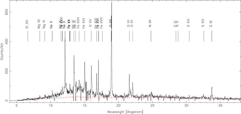
Figure 2: RGS 1 first order spectrum of AB Dor from the revolution #091 observation. The dashed line represents the continuum predicted by the EMD. A false continuum is created by the extended instrumental line profiles.

As one of the brightest X-ray stellar sources, AB Dor has been chosen for the XMM-Newton calibration program, and 15 observations are available to date, totalling 594 ks of clean RGS spectra. This is the first of a series of papers devoted to a detailed and systematic analysis of the XMM-Newton observations available to date, and it is dedicated to the high resolution spectra with the lowest and highest global count rates, with the aim of understanding the properties of the corona of AB Dor in two different activity levels. In this paper we also present the result of a new analysis of the higher resolution Chandra/HETG spectrum, performed with the same method employed for the XMM data. Issues related to the analysis of XMM/RGS and Chandra/HETG spectra are discussed, and a comparison with the results obtained from previous EUVE observations is presented.

The technical information related to the observations is given in Sect. 2. The methods employed to analyze the data are delineated in Sect. 3, as well as the issues that may affect the measurements in this kind of spectra. The scientific results are discussed in Sect. 4, followed by a summary of the conclusions in Sect. 5.

2 Observations

2.1 XMM-Newton

AB Dor has been frequently observed as XMM-Newton calibration target since May 2000 (Table 1), with different combinations of instruments operating simultaneously. XMM-Newton allows to carry out simultaneous observation with the EPIC (European Imaging Photon Camera) PN and MOS detectors (sensitivity range 0.15–15 keV and 0.2–10 keV respectively), and with the RGS (Reflection Grating Spectrometer, den Herder et al., 2001) ($\lambda\lambda\sim$6–38 Å), allowing us to obtain simultaneously medium-resolution CCD spectra ($\Delta E\sim$70 eV at $E\sim$1 keV) and high-resolution grating ($\lambda$/$\Delta\lambda\sim$100–500) spectra. The data have been reduced by employing the standard tasks present in the SAS (Science Analysis Software) package v5.3.3, removing the time intervals when the background was higher than 0.5 cts/s in CCD #9, in order to ensure a “clean” spectrum. The average count rates obtained in the RGS 2 spectra, after the high-background removal, are shown in Table 1. The observations with the lowest and highest RGS count rates (rev. #091 and rev. #205) are analyzed in detail in this work in order to investigate the differences in the coronal thermal structure among these two levels of activity. Light curves for the two observations (Fig. 1a and b) were obtained by selecting a circle centered on the source in the EPIC-pn images, and subtracting the background count rate taken proportionally. The image presents a clear asymmetry in the main source, that we attribute to AB Dor B; this source can contaminate both the light curve and the RGS spectra of AB Dor, but we can safely neglect its effects in the RGS spectra, given the flux ratio observed with Chandra (see below). High resolution spectra corresponding to the first order of the RGS (Fig. 2), together with some of the lines identified, are analyzed as explained in Sect. 3. Second order RGS spectra have been used to double check for the blends contributing to the main lines (Fig. 3), and to test the flux calibration with respect to the first order (see Sect. 3.1).

2.2 Chandra

AB Dor was observed on 9 October 1999 for 52 ks with the Chandra High Energy Transmission Grating Spectrograph, (HETG, Weisskopf et al., 2002). The HETGS is made of two gratings, HEG (High Energy Grating, $\lambda\lambda\sim$1.5–15, $\lambda/\Delta\lambda\sim$120–1200), and MEG (Medium Energy Grating $\lambda\lambda\sim$3–30, $\lambda/\Delta\lambda\sim$60–1200), that operate simultaneously, permitting the further analysis of the data with different spectral resolutions. Standard reduction tasks present in the CIAO v2.3 package have been employed in the reduction of data retrieved from the Chandra archive, and the extraction of the HEG and MEG spectra (Fig. 4). Two sources are visible in the CCD image at their zero-order positions. The main source ($\alpha$=5:28:44.8, $\delta$=–65:26:55.5) is identified as AB Dor, while the second source ($\alpha$=5:28:44.4 $\delta$=–65:26:46.5) agrees with the position of AB Dor B (dM4e). A light curve of AB Dor A+B was obtained using the first orders of HEG and MEG (Fig. 1c), while the zeroth-order was employed to get a light curve of the secondary source alone (the zeroth-order of the primary source is severely affected by pile-up). No significant flaring events are present in the light curve of AB Dor B, and a low-resolution ACIS-S spectrum (sensitivity range 0.4–10.0 keV, $E/\Delta E\sim$50 at 6 keV) was obtained for it (see Sanz-Forcada et al., 2003b, for further details). This spectrum was employed to calculate the flux in the range 6–25 Å ($f_{\rm X}\sim$1.26$\times$10^-12 erg s^-1 cm^-2, $L_{\rm X}\sim$3.35$\times$10²⁸ erg s^-1). The flux of AB Dor A+B calculated in the same spectral range of the MEG spectra is $f_{\rm X}\sim$2.75$\times$10^-11 erg s^-1 cm^-2, $L_{\rm X}\sim$7.35$\times$10³⁰ erg s^-1, therefore the secondary source only represents $\sim$4% of the total flux of the system. A 3-temperature global fit was made to the low-resolution spectrum of AB Dor B (Sanz-Forcada et al., 2003b) using the Astrophysical Plasma Emission Database (APED v1.3, Smith et al., 2001) in the Interactive Spectral Interpretation System (ISIS, Houck & Denicola, 2000) software package, provided by the MIT/CXC, and a synthetic MEG spectrum was constructed based on this fit. The comparison of this synthetic spectrum with the total MEG spectrum shows that the effects of AB Dor B on the total spectrum are negligible (both for HETG and XMM/RGS spectra).

Table 1: XMM observations of AB Dor

Rev.	Date	pn	mos	RGS	RGS 2
				$t_{\rm exp}$(ks)	cts/s
072	1 May 2000	X	–	40+12	1.14
091	7 Jun 2000	X	–	54	1.01
162	27 Oct 2000	X	X	57	1.22
185	11 Dec 2000	X	X	56+8+20	1.37
205	20 Jan 2001	X	X	51	1.77
266	22 May 2001	X	X	48	1.24
338	10 Oct 2001	–	X	38	1.21
375	26 Dec 2001	–	X	4	1.28
429	12 Apr 2002	X	X	43	1.07
462	18 Jun 2002	X	X	35	1.51
532	5 Nov 2002	–	–	9	1.60
537	15 Nov 2002	–	X	15	1.59
546	3 Dec 2002	X	X	4	1.60
560	30 Dec 2002	–	X	49	1.57
572	23 Jan 2003	–	–	51	1.15

Finally, the emission level of AB Dor at the time of the Chandra observation of AB Dor has been compared with the RGS 2 count rates by folding the Emission Measure Distribution based on the Chandra spectra (see below) with the RGS instrumental response. This simulation yields a count rate of $\sim$1.01 cts/s, consistent with the count rate obtained in the RGS #091 observation. Further analysis of the light curves and the long-term variability of the Chandra and XMM observations of AB Dor will follow in Sanz-Forcada et al. (2003b).

3 Data Analysis

Stellar coronae are commonly studied through the calculation of the coronal thermal structure. Such a structure is derived by using the plasma Emission Measure Distribution vs. Temperature (EMD), with the volume Emission Measure $EM$($T$) defined as $\int_{\Delta T}N_{H}N_{e}{\rm d}V$ [cm^-3]. The $EM$ quantifies how much material is emitting in a temperature range $\Delta T$, and it can be used to compute the radiative losses in corona and hence to get information on the required coronal heating. Two different approaches are commonly employed in the derivation of the EMD in the corona: line-based methods and global-fitting techniques. The latter are based on the fit of the whole (lines plus continuum) spectrum using an atomic model and a discrete number of values of temperature and $EM$. Such an approach uses the metallicity (or even the abundances of individual elements) as free parameters in the fit. An alternative method, that can be carried out only for high-resolution spectra, implies the measurement of individual line fluxes and its comparison with the fluxes predicted by an atomic model for a given EMD (“line-based” methods, or “EMD reconstruction”). The application of these two approaches, although never directly compared, seems to yield different results, especially regarding the element abundances (Favata & Micela, 2003). In this work we will apply a line-based method to reconstruct the EMD of the corona of AB Dor in intervals of 0.1 dex in temperature. We have performed also a global fit to the spectra, with the aim to compare the results derived with the two techniques.

Figure 3: RGS 1 second order spectrum of AB Dor from the rev. #091 observation.

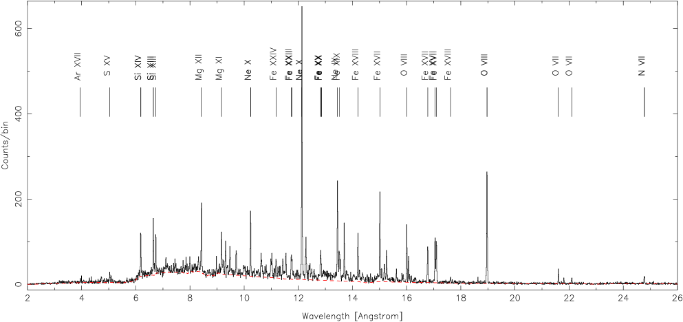
Figure 4: Chandra/MEG spectrum of AB Dor. The dashed line represents the continuum predicted by the EMD.

3.1 EMD reconstruction

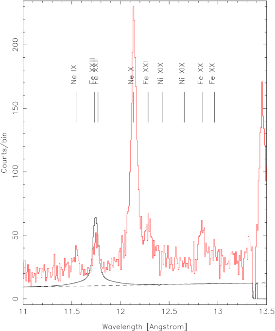
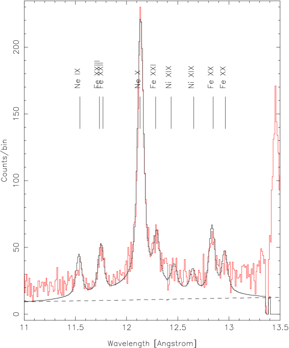
Figure 5: Section of the RGS 2 spectrum of rev. # 091, showing the fit to the line Fe xxiii $\lambda$11.736 alone (left), and including important lines in the same wavelength region (right). The flux measured for the Fe xxiii $\lambda$11.736 line is a 43% higher if the additional lines considered in the right panel are not included in the fit. The presence of a false continuum created by the LSF of adjacent lines influences the measurement of every line. A dashed line indicates the continuum predicted from the EMD.

The EMD reconstruction has been carried out by measuring the fluxes from spectral lines present in the RGS and HETG spectra. RGS spectra are characterized by a Line Spread Function (LSF) with particularly extended wings that, if not properly taken into account, may result in a wrong measurement of the lines fluxes (see an example in Fig. 5). The extended wings of the lines also create a false continuum that makes difficult the placement of the real source continuum to be used when line fluxes are measured (this is especially problematic in the 9–18 Å range, where numerous lines overlap, see Fig. 2). Such a problem has been solved by using an iterative process as explained below. The same process (partly similar to the method described by Huenemoerder et al., 2001) has been applied to the HETG spectral analysis, where the problems related to the shape of the LSF are less severe. Line fluxes from 108 lines, with their corresponding line blends (Table 2), have been considered in the analysis of HETG spectra, while 59 lines were used for the RGS spectra as listed in Table 3. Spectra, response matrices and the effective areas of the instruments, were loaded into the ISIS software package, in order to measure the line fluxes, following the procedure here described:

– A two-temperatures fit to the continuum is made in the case of HETG, using line-free regions only, as described in Huenemoerder et al. (2001) and Brickhouse (2001). This fit yields an initial estimate of the continuum, needed for the line measurements. In the case of RGS spectra, where line-free regions are more difficult to measure, a global 2-T fit to the spectrum is performed to calculate the initial continuum level.

– Measurements of line fluxes are made using the continuum predicted with the former fit, and convolving delta functions with the Line Response Function of the instrument. Simultaneous fit of the MEG and HEG spectra were carried out when possible, while separated measurements were made for RGS 1 and RGS 2 spectra. Initial line identification with atomic data from APED v1.3, is made on the basis of the Emission Measure Distribution (EMD) derived by Sanz-Forcada et al. (2002) from EUVE data. The false continuum created by the LSF of numerous lines in the range 9–18 Å of RGS (see Fig. 5), makes more difficult the measurement of lines in this spectral range; a fit involving the most intense adjacent lines for each of the line measurements was necessary in order to obtain results of the EMD that were consistent with the spectra. Much care has to be considered in the measurement of any line in this spectral range of RGS.

– Predicted fluxes are calculated using the emissivity functions present in APED and a trial EMD (the EUVE based EMD mentioned above is employed initially in this case), following the method described in Dupree et al. (1993). The quality of the fit is tested with the parameter $\beta$, defined as:

$$\beta=\frac{1}{n}\sum_{i=1}^{n}\Big{(}\log\frac{F_{\mathrm{obs},i}}{F_{\mathrm{pred},i}}\Big{)}^{2}$$ (1)

where n is the number of lines considered, $F_{\mathrm{obs}}$ are the fluxes measured in the spectra and $F_{\mathrm{pred}}$ are the fluxes predicted by combining the assumed EMD and the APED atomic models (a “perfect” fit would yield $\beta$=0). Only Fe lines are initially employed, thus avoiding uncertainties due to relative abundances. Line blends that may affect the main lines must be included in the analysis. Predicted fluxes are then compared to observed fluxes in order to improve the EMD.

Table 2: Chandra/HETG line fluxes of AB Dor^a

Ion	$\lambda$model	$\lambda$obs	log $T_{\mathrm{max}}$	$F_{\mathrm{obs}}$	S/N	ratio	Blends
Ar xvii	3.9491	3.949	7.3	4.62e-14	4.6	-0.00
S xvi	3.9908	3.988	7.4	3.59e-14	4.1	0.05	S xvi 3.9920, Ar xvii 3.9941, 3.9942, S xv 3.9980
S xv	4.2990	4.290	7.2	3.95e-14	4.3	0.29
S xvi	4.7274	4.732	7.4	5.92e-14	5.3	-0.06	S xvi 4.7328
S xv	5.0387	5.039	7.2	1.05e-13	7.1	-0.13
S xv	5.1015	5.100	7.2	4.90e-14	4.8	-0.12	S xv 5.0983, 5.1025
Si xiv	5.2168	5.213	7.2	2.09e-14	3.0	0.03	Si xiv 5.2180
Si xiv	6.1804	6.183	7.2	1.47e-13	16.4	0.06	Si xiv 6.1804, 6.1858
Mg xii	6.5800	6.530	7.0	1.36e-14	5.4	0.38	Fe xxiv 6.5772, Mg xii 6.5802
Si xiii	6.6479	6.648	7.0	1.42e-13	17.3	-0.06
Si xiii	6.6882	6.687	7.0	2.62e-14	7.5	-0.07	Si xiii 6.6850
No id.	6.7120	6.715	…	1.55e-14	5.8	…
Si xiii	6.7403	6.741	7.0	9.77e-14	15.7	0.07	Mg xii 6.7378, Si xiii 6.7432
Mg xii	7.1058	7.106	7.0	2.79e-14	8.8	-0.05	Mg xii 7.1069
Al xiii	7.1710	7.168	7.1	1.97e-14	7.4	0.00	Fe xxiv 7.1690, Al xiii 7.1764
Mg xi	7.4730	7.478	6.8	1.10e-14	5.6	0.23
Mg xi	7.8503	7.858	6.8	2.60e-14	8.5	0.14
Fe xxiv	7.9857	7.987	7.3	2.22e-14	8.4	0.20	Fe xxiv 7.9960
Fe xxiii	8.3038	8.309	7.2	2.36e-14	9.6	0.23
Fe xxiv	8.3761	8.377	7.3	9.81e-15	3.2	0.33
Mg xii	8.4192	8.416	7.0	1.32e-13	20.5	-0.18	Mg xii 8.4246
Fe xxii	8.9748	8.974	7.1	2.30e-14	7.8	0.15
Ni xxvi	9.0603	9.075	7.4	1.39e-14	6.3	-0.02	Fe xxii 9.0614, Fe xx 9.0647, 9.0659, 9.0683
No id.	9.1300	9.135	…	9.27e-15	5.1	…
Mg xi	9.1687	9.170	6.8	8.85e-14	15.8	-0.16
Fe xxi	9.1944	9.193	7.1	1.85e-14	7.2	0.26	Mg xi 9.1927, 9.1938, Fe xx 9.1979
No id.	9.2190	9.216	…	1.25e-14	5.9	…	Ne x 9.215
Mg xi	9.2312	9.234	6.8	2.19e-14	7.8	-0.02	Mg xi 9.2282
Ni xix	9.2540	9.251	6.9	8.05e-15	4.7	0.24
No id.	9.2870	9.291	…	1.47e-14	6.4	…	Ne x 9.291
Mg xi	9.3143	9.315	6.8	4.74e-14	11.5	-0.03
No id.	9.3600	9.357	…	1.24e-14	5.9	…
Ni xx	9.3850	9.389	7.0	1.93e-14	7.3	0.28	Ni xxvi 9.3853, Ni xxv 9.3900, Fe xxii 9.3933
Fe xxi	9.4797	9.473	7.0	3.95e-14	10.4	-0.16	Ne x 9.4807, 9.4809
Ne x	9.7080	9.705	6.8	6.20e-14	12.8	-0.14	Ne x 9.7085
Ni xix	9.9770	9.973	6.9	4.46e-14	10.6	-0.12	Ni xxv 9.9700, Fe xxi 9.9887, Fe xx 9.9977, 10.0004, 10.0054
No id.	10.0200	10.025	…	1.93e-14	6.9	…
Fe xx	10.1203	10.113	7.0	2.04e-14	7.1	-0.02	Ni xix 10.1100, Fe xix 10.1195, Fe xvii 10.1210
Ne x	10.2385	10.238	6.8	1.55e-13	19.3	-0.17	Ne x 10.2396
Fe xxiv	10.6190	10.625	7.3	5.65e-14	11.2	-0.01	Fe xix 10.6295
Fe xix	10.6491	10.645	6.9	2.67e-14	7.7	0.07	Fe xix 10.6414
Fe xxiv	10.6630	10.665	7.3	2.70e-14	7.7	-0.12	Fe xvii 10.6570
Fe xvii	10.7700	10.765	6.8	2.34e-14	7.2	-0.05	Ne ix 10.7650, Fe xix 10.7650
Fe xix	10.8160	10.818	6.9	2.46e-14	7.3	0.06
Fe xxiii	10.9810	10.985	7.2	4.32e-14	9.5	-0.13
Ne ix	11.0010	11.005	6.6	3.06e-14	8.0	0.12	Ni xxii 10.9920, 10.9927
Fe xxiv	11.0290	11.035	7.3	6.73e-14	11.8	-0.08	Fe xxiii 11.0190, Fe xvii 11.0260
Fe xvii	11.1310	11.128	6.8	1.84e-14	6.1	-0.09	Fe xxii 11.1376
Fe xxiv	11.1760	11.175	7.3	6.28e-14	11.2	-0.05	Fe xxiv 11.1870
Fe xvii	11.2540	11.252	6.8	3.25e-14	8.0	-0.14	Fe xxiv 11.2680
Ni xxii	11.3049	11.303	7.1	2.37e-14	6.8	0.17	Fe xviii 11.2930, Fe xix 11.2980, Ni xxi 11.3180
Fe xviii	11.3260	11.325	6.9	3.18e-14	7.8	-0.07	Fe xxiii 11.3360
Fe xviii	11.4230	11.423	6.9	4.94e-14	9.5	0.02	Fe xxii 11.4270
Fe xxiv	11.4320	11.435	7.3	3.39e-14	7.7	0.01
Fe xxii	11.4900	11.495	7.1	2.52e-14	6.6	0.03
Fe xviii	11.5270	11.527	6.9	3.83e-14	8.2	0.09
Ne ix	11.5440	11.543	6.6	6.28e-14	10.5	0.06
Fe xxiii	11.7360	11.740	7.2	7.67e-14	11.4	-0.19
Fe xxii	11.7700	11.773	7.1	7.12e-14	10.8	-0.22
Fe xxii	11.8020	11.796	7.1	1.62e-14	5.1	0.14
Ni xx	11.8320	11.818	7.0	1.80e-14	5.5	0.04
Fe xxii	11.9320	11.937	7.1	2.92e-14	7.0	0.16
Fe xxii	11.9770	11.973	7.1	2.87e-14	6.9	-0.07	Fe xxi 11.9750
Ne x	12.1321	12.133	6.8	9.43e-13	39.2	-0.19	Fe xvii 12.1240, Ne x 12.1375
Fe xxiii	12.1610	12.158	7.2	7.83e-14	11.3	0.08
Fe xxii	12.2100	12.210	7.1	1.99e-14	5.6	0.02
Fe xvii	12.2660	12.268	6.8	6.61e-14	10.2	0.01
Fe xxi	12.2840	12.288	7.0	1.44e-13	15.1	-0.02
Fe xxi	12.3930	12.398	7.0	4.99e-14	8.8	0.23	Fe xxi 12.3940
Fe xxi	12.4220	12.429	7.0	4.53e-14	8.3	-0.43	Fe xxii 12.4311, 12.4318, Ni xix 12.4350
Fe xxi	12.4990	12.496	7.0	3.70e-14	7.5	0.14	Fe xxi 12.4956
No id.	12.8100	12.813	…	6.70e-14	9.7	…
Fe xx	12.8240	12.829	7.0	1.55e-13	14.7	-0.31	Fe xxi 12.8220, Fe xx 12.8460, Fe xx 12.8640
Fe xx	12.9650	12.943	7.0	4.09e-14	7.5	-0.13	Fe xxii 12.9530
Ne ix	13.4473	13.448	6.6	4.94e-13	24.5	0.10	Fe xix 13.4620
Fe xxi	13.5070	13.508	7.0	1.15e-13	11.7	0.11	Fe xix 13.4970
Fe xix	13.5180	13.518	6.9	9.93e-14	10.9	-0.11
Fe xx	13.5350	13.535	7.0	3.03e-14	6.0	0.19
Ne ix	13.5531	13.550	6.6	9.67e-14	10.7	0.18	Fe xix 13.5510, 13.5540, Fe xx 13.5583
Ne ix	13.6990	13.700	6.6	2.61e-13	16.9	0.17	Fe xix 13.7315, and small blends amounting a 15% of total flux.
Ni xix	13.7790	13.768	6.8	3.91e-14	6.5	-0.18	Fe xx 13.7670
Fe xix	13.7950	13.795	6.9	5.29e-14	7.6	-0.04

Table 2: (cont). Chandra/HETG line fluxes of AB Dor^a

Ion	$\lambda$model	$\lambda$obs	log $T_{\mathrm{max}}$	$F_{\mathrm{obs}}$	S/N	ratio	Blends
Fe xvii	13.8250	13.815	6.8	2.19e-14	4.9	-0.32
Fe xix	13.8390	13.835	6.9	3.92e-14	6.5	0.21	Fe xx 13.8430
Fe xviii	13.9530	13.954	6.9	1.37e-14	3.8	-0.42	Fe xix 13.9549, 13.9551, Fe xx 13.9620
Fe xxi	14.0080	14.015	7.0	3.20e-14	5.7	0.12
Ni xix	14.0430	14.045	6.8	3.27e-14	5.9	-0.08
Ni xix	14.0770	14.073	6.8	3.25e-14	5.9	-0.04
Fe xviii	14.2080	14.205	6.9	2.38e-13	15.6	-0.06
Fe xviii	14.2560	14.257	6.9	7.12e-14	8.5	-0.10	Fe xx 14.2670
Fe xviii	14.3430	14.345	6.9	3.20e-14	5.0	-0.09
Fe xviii	14.3730	14.372	6.9	6.62e-14	7.2	-0.02
Fe xviii	14.5340	14.535	6.9	5.64e-14	6.5	0.04
Fe xix	14.6640	14.675	6.9	5.34e-14	6.3	0.17
O viii	14.8205	14.815	6.5	2.64e-14	5.0	-0.06
Fe xx	14.9703	14.970	7.0	3.11e-14	5.9	0.02	Fe xix 14.9610
Fe xvii	15.0140	15.014	6.7	4.37e-13	21.9	-0.08
Fe xx	15.0470	15.044	7.0	2.85e-14	5.6	0.37
Fe xix	15.0790	15.078	6.9	6.72e-14	8.5	0.21
O viii	15.1760	15.173	6.5	6.23e-14	8.2	-0.23	O viii 15.1765
Fe xix	15.1980	15.190	6.9	9.50e-14	10.1	0.44
Fe xvii	15.2610	15.259	6.7	2.04e-13	14.6	0.13
Fe xvii	15.4530	15.455	6.7	2.39e-14	4.9	0.16
Fe xviii	15.6250	15.620	6.8	6.68e-14	8.1	0.00
Fe xviii	15.8240	15.831	6.8	5.53e-14	7.2	0.14
Fe xviii	15.8700	15.860	6.8	2.49e-14	4.9	0.03
O viii	16.0055	16.005	6.5	3.36e-13	17.6	-0.06	Fe xviii 16.0040, O viii 16.0067
Fe xviii	16.0710	16.071	6.8	1.63e-13	12.2	0.27
Fe xix	16.1100	16.105	6.9	3.66e-14	5.8	-0.14	Fe xviii 16.1127
Fe xviii	16.1590	16.158	6.8	5.07e-14	6.8	0.14
Fe xvii	16.7800	16.775	6.7	2.80e-13	15.2	0.10
Fe xvii	17.0510	17.053	6.7	3.67e-13	17.0	0.19
Fe xvii	17.0960	17.095	6.7	3.46e-13	16.4	0.26
Fe xviii	17.6230	17.620	6.8	5.35e-14	6.1	-0.03
O vii	18.6270	18.635	6.3	4.16e-14	5.0	0.12	Ar xvi 18.6240
Ca xviii	18.6910	18.694	6.9	1.19e-14	2.6	-0.30
O viii	18.9671	18.967	6.5	1.28e-12	26.6	-0.11	O viii 18.9725
O vii	21.6015	21.608	6.3	2.23e-13	8.6	0.09
O vii	21.8036	21.805	6.3	7.92e-14	4.9	0.17
O vii	22.0977	22.095	6.3	1.39e-13	6.1	0.21	Ca xvii 22.1140
N vii	24.7792	24.779	6.3	1.31e-13	7.2	0.00	N vii 24.7846

^a Line fluxes (in erg cm^-2 s^-1) of spectral lines measured in Chandra/HETG spectra. Measured wavelengths (in Å) are accurate to $\sim 10^{-3}$ Å. log $T_{\mathrm{max}}$ indicates the maximum temperature (K) of formation of the line (unweighted by the EMD). “Ratio” is the log($F_{\mathrm{obs}}$/$F_{\mathrm{pred}}$) of the line. Blends amounting to more than 5% of the total flux on each line are indicated.

Table 3: XMM line fluxes of AB Dor^a

			XMM rev. 091			XMM rev. 205
Line ID	$\lambda$model	log Tmax	$F_{\mathrm{obs}}$	S/N	ratio	$F_{\mathrm{obs}}$	S/N	ratio	Blends
Si xiv	6.1804	7.2	1.38e-13	3.0	0.25	2.37e-13	5.5	0.08
Si xiii	6.6480	7.0	3.17e-13	6.1	0.01	5.35e-13	8.2	-0.09	Si xiii 6.6882, 6.7403
Mg xii	8.4192	7.0	1.52e-13	7.3	-0.04	4.25e-13	13.0	0.00
Mg xi	9.1687	6.8	9.60e-14	13.8	-0.13	2.10e-13	19.4	-0.13
Mg xi	9.2312	6.8	1.56e-13	8.1	0.20	3.06e-13	10.5	0.17	Ni xix 9.2540, Mg xi 9.3143
Ne x	9.7080	6.8	1.06e-13	7.6	-0.08	2.44e-13	11.4	0.02
Ne x	10.2385	6.8	2.28e-13	13.8	-0.15	4.41e-13	18.1	-0.12
Fe xxiv	10.6190	7.3	1.41e-13	5.8	0.11	2.71e-13	7.4	0.07	Fe xix 10.6491, 10.6840, Fe xxiv 10.6630
Fe xvii	10.7700	6.8	8.34e-14	5.9	0.12	1.76e-13	5.3	0.22	Fe xix 10.8160
Fe xxiii	11.0190	7.2	1.50e-13	11.1	0.03	3.46e-13	11.6	0.03	Fe xxiii 10.9810, Ne ix 11.0010, Fe xxiv 11.0290
Fe xxiv	11.1760	7.3	1.21e-13	9.8	0.19	1.66e-13	6.8	-0.02	Fe xvii 11.1310
Fe xvii	11.2540	6.8	…	…	…	1.60e-13	6.7	0.23	Fe xxiii 11.2850
Fe xviii	11.4230	6.9	9.49e-14	7.9	0.04	2.55e-13	9.5	0.13	Fe xxiv 11.4320, Fe xviii 11.4494, Fe xxiii 11.4580
Fe xviii	11.5270	6.9	1.55e-13	11.3	0.00	2.11e-13	8.2	-0.11	Fe xxii 11.4900, Ni xix 11.5390, Ne ix 11.5440
Fe xxiii	11.7360	7.2	2.35e-13	15.5	0.10	5.09e-13	16.1	0.01	Fe xxii 11.7700
Ne x	12.1321	6.8	1.40e-12	50.3	0.02	2.34e-12	52.9	-0.22
Fe xxi	12.2840	7.0	2.33e-13	14.4	0.05	5.20e-13	12.7	0.07	Fe xvii 12.2660
Ni xix	12.4350	6.9	1.23e-13	10.0	-0.19	2.09e-13	8.0	-0.13	Fe xxi 12.3930, 12.4220
Fe xxi	12.4990	7.0	…	…	…	1.87e-13	7.8	0.11	Fe xx 12.5260, 12.5760
Fe xxi	12.6490	7.0	7.78e-14	7.4	0.17	1.45e-13	6.7	0.30	Fe xx 12.6210, Fe xxii 12.6307, Ni xix 12.6560
Fe xx	12.8240	7.0	2.83e-13	18.9	-0.05	5.73e-13	18.1	-0.04
Fe xx	12.9650	7.0	1.62e-13	13.0	0.01	3.52e-13	12.5	0.06	Fe xx 12.9120, 12.9920, 13.0240, Fe xix 12.9330, 13.0220
Ne ix	13.4473	6.6	7.72e-13	40.6	0.10	1.11e-12	45.7	0.02	Fe xx 13.3850
Fe xix	13.5180	6.9	3.00e-13	22.2	-0.08	7.01e-13	36.7	0.04	Fe xxi 13.5070, Ne ix 13.5531
Ne ix	13.6990	6.6	4.25e-13	16.2	0.14	7.04e-13	20.1	0.15	Fe xix 13.6450, 13.7315, 13.7458
Fe xix	13.7950	6.9	1.95e-13	14.2	-0.00	1.60e-13	9.0	-0.28	Ni xix 13.7790, Fe xvii 13.8250
Fe xx	13.9620	7.0	7.23e-14	6.8	0.10	8.48e-14	7.8	-0.07	Fe xviii 13.9530, Fe xix 13.9525, 13.9546, 13.9571, 13.9743
Fe xxi	14.0080	7.0	1.62e-13	8.7	-0.00	1.69e-13	10.9	-0.11	Fe xix 14.0340, 14.0717, Ni xix 14.0430, 14.0770
Fe xviii	14.2080	6.9	4.03e-13	21.2	-0.04	6.34e-13	26.4	-0.06	Fe xviii 14.2560
Fe xviii	14.3730	6.9	1.72e-13	14.1	-0.11	2.57e-13	19.7	-0.16	Fe xx 14.3318, 14.4207, Fe xviii 14.3430, 14.4250, 14.4392
Fe xviii	14.5340	6.9	1.89e-13	12.5	0.17	2.91e-13	18.4	0.15	Fe xviii 14.4856, 14.5056, 14.5710, 14.6011
O viii	14.8205	6.5	8.62e-14	8.9	0.06	1.45e-13	10.3	0.00	Fe xviii 14.7820, O viii 14.8207, Fe xx 14.8276
Fe xvii	15.0140	6.7	6.08e-13	32.8	-0.10	9.49e-13	37.5	-0.14	Fe xix 15.0790
O viii	15.1760	6.5	1.91e-13	15.1	0.04	3.17e-13	16.9	-0.02	Fe xix 15.1980
Fe xvii	15.2610	6.7	2.02e-13	18.7	0.05	3.59e-13	22.6	0.07
Fe xviii	15.6250	6.8	8.21e-14	9.5	0.01	1.57e-13	12.5	0.08
Fe xviii	15.8700	6.8	1.20e-13	10.7	0.20	1.83e-13	13.3	0.17	Fe xviii 15.8240
O viii	16.0066	6.5	3.71e-13	29.9	-0.12	6.71e-13	32.6	-0.14	O viii 16.0055
Fe xviii	16.0710	6.8	1.88e-13	15.9	-0.06	2.89e-13	16.2	-0.09	Fe xviii 16.0450, 16.1590, Fe xix 16.1100, 16.1590
Fe xvii	16.7800	6.7	2.93e-13	22.4	0.03	4.58e-13	26.6	-0.00
Fe xvii	17.0510	6.7	7.11e-13	36.9	0.13	1.03e-12	50.1	0.07	Fe xvii 17.0960
Fe xviii	17.6230	6.8	6.80e-14	9.1	-0.01	1.31e-13	12.4	0.07
O vii	18.6270	6.3	3.91e-14	5.7	-0.25	1.19e-13	10.5	-0.18	Ca xviii 18.6910
O viii	18.9671	6.5	1.33e-12	54.4	-0.20	2.91e-12	79.2	-0.16
N vii	20.9095	6.3	4.06e-14	4.7	0.05	5.13e-14	4.6	-0.02	N vii 20.9106
Ca xvi	21.4500	6.7	2.02e-14	7.2	0.11	7.14e-14	6.2	0.14	Ca xvi 21.4410
O vii	21.6015	6.3	2.99e-13	27.7	0.08	5.24e-13	22.0	0.08	Ca xvi 21.6100
O vii	21.8036	6.3	9.69e-14	8.7	0.18	1.60e-13	10.7	0.16	Ca xvii 21.8220
O vii	22.0977	6.3	1.77e-13	12.9	0.17	3.38e-13	16.8	0.19	Ca xvii 22.1140
Ar xvi	23.5460	6.7	3.57e-14	2.9	0.16	4.92e-14	3.6	-0.15	Ar xvi 23.5900, Ca xvi 23.6260
N vii	24.7792	6.3	2.18e-13	21.8	-0.04	3.80e-13	28.9	0.03	Ar xvi 24.8540
Ar xvi	24.9910	6.7	1.71e-14	2.6	-0.15	6.44e-14	11.5	0.00	Ar xvi 25.0130, Ar xv 25.0500
C vi	26.9896	6.2	2.66e-14	5.7	0.29	4.44e-14	6.9	0.18	C vi 26.9901
C vi	28.4652	6.2	2.48e-14	5.3	-0.20	7.48e-14	9.8	-0.05	C vi 28.4663
S xiv	30.4270	6.5	2.93e-14	5.6	-0.18	4.77e-14	6.9	-0.14	S xiv 30.4690, Ca xi 30.4710
S xiv	32.4160	6.5	2.13e-14	3.1	0.15	3.07e-14	3.4	0.20
S xiv	32.5600	6.5	3.93e-14	4.8	0.12	4.69e-14	4.7	0.09	S xiv 32.5750
C vi	33.7342	6.1	1.86e-13	17.8	-0.08	3.54e-13	24.1	-0.12	C vi 33.7396

^a Line fluxes (in erg cm^-2 s^-1) of spectral lines measured in XMM/RGS first order spectra. log $T_{\mathrm{max}}$ indicates the maximum temperature (K) of formation of the line (unweighted by the EMD). “Ratio” is the log($F_{\mathrm{o}bs}$/$F_{\mathrm{pred}}$) of the line. Blends amounting to more than 5% of the total flux for each line are indicated (see also blends in Table 2).

– Once the $\beta$ parameter converges to a minimum value, neon lines are added to the analysis in order to extend the EMD to lower temperatures. The Ne x lines are mostly formed in a temperature range (log $T$[K]$\sim$6.6–7.3) which overlaps with that of the Fe lines, therefore permitting to set the Ne abundance. Then, the oxygen abundance can be set employing the O viii lines, and the O vii lines provide information down to log $T$(K)$\sim$6.2. Finally, the rest of the elements (Mg, S, Si, Ar, Ni, N, Ca, C, Al) are added one by one in the analysis, in order to calculate the abundances (relative to Fe) that better fit their fluxes, leaving the EMD unchanged.

– The continuum is recomputed, and new flux measurements are performed. Changes of the EMD shape are now permitted, once all elements are included in the fit. An iterative process is followed until the measurements of the lines converge. Electron densities (see below) are included in the analysis by applying the relevant values in their corresponding temperature ranges (log $T$[K]$\sim$6.1–6.4 for density derived from O vii lines, log $T$[K]$\sim$6.5–6.6 for density from Ne ix lines, and log $T$[K]$\sim$6.7–7.2 for density from Mg xi, Fe xxi and Fe xxii line ratios). The Fe abundance is determined once the EMD has been calculated, and the rest of abundances are scaled to the [Fe/H] value.

Statistical uncertainties on the EMD values (Table 4), are estimated using a Montecarlo method that varies the line fluxes randomly by 1–$\sigma$ (1000 different sets of fluxes are tested), and calculates the best result among 1000 possible EMDs (randomly generated, including variations by up to 1–$\sigma$ over the calculated abundances) for each pattern of fluxes. A criterion of convergence is established in the improvement of $\beta$ by at least 5$\times 10^{-4}$. The 68% of the central values among those resulting from this fit, are considered in order to set the 1–$\sigma$ error bars of the $EM$ values. These error bars are not independent, a higher value of the $EM$ in a given temperature bin usually requires a lower value in an adjacent bin in order to match the observed line fluxes. Finally, uncertainties in the determination of the abundances (Table 6) are evaluated considering not only the statistical errors of the measured fluxes, but also the dispersion observed in the $F_{\mathrm{obs}}/F_{\mathrm{pred}}$ ratio of all the lines of each element. This is an indirect way to evaluate the errors induced by the uncertainties in atomic models.

The results obtained in the RGS rev. #091 are consistent with those of the HETG observation. The bump present at log $T$(K)$\sim$6.9 is very robust in both cases (see Table 4). The presence of a hot tail is well established for log $T$(K)$\sim$7.0–7.3, with some uncertainties on the exact shape. Larger error bars in the EMD are present at log $T$(K)$\la$6.6, due to the lack of Fe lines that would reduce the uncertainties in the abundances of Ne and O. Fe xv and Fe xvi lines formed at those temperatures are well observed with EUVE (Sanz-Forcada et al., 2002) for AB Dor, and can be used (with some caution) for a consistency test of the results. However, these lines are affected by uncertainties in the determination of the ISM absorption, and the EUVE spectrum could correspond to a different level of emission. The formal solution, shown in Figs. 6 and 7 and Table 4, has been a compromise of the results found for the Ne lines and the mentioned EUVE lines, that are overestimated by up to $\sim$50% with the solution derived from HETG spectra. Finally, abundances of elements like Ca, Al and Ar are not very robust since they are derived from little number of lines. Also, C and N lines present in the spectra have a temperature range that overlaps mostly with that of O vii, and hence the abundances of C and N are linked to that of O. Marginal inconsistency in the abundances calculated from RGS and HETG detectors is only found for Ca, N and Ne.

The measurements of line fluxes in the RGS spectra during rev. #205 yield an EMD with similar shape to that of HETG and RGS rev.#091, but with higher $EM$ values. Abundances of the elements did not change significantly between the two RGS observations, except for the worse constrained cases of Ca and N. Finally, the line fluxes have been measured in the second order of RGS during rev. #091 (Table 5), resulting in a very good agreement with the EMD and abundances calculated with the first order of RGS (Fig. 8).

Table 4: Emission Measure Distribution of AB Dor

log $T$	log $\int N_{\rm e}N_{\rm H}{\rm d}V$ (cm-3)a
(K)	HETG	RGS 091	RGS 205
6.1	50.27:	50.37:	50.47:
6.2	50.57${}^{+0.30}_{-0.20}$	50.57${}^{+0.20}_{-0.20}$	50.67${}^{+0.15}_{-0.35}$
6.3	50.67${}^{+0.20}_{-0.20}$	50.67${}^{+0.15}_{-0.25}$	50.77${}^{+0.10}_{-0.30}$
6.4	50.47${}^{+0.20}_{-0.30}$	50.37${}^{+0.30}_{-0.40}$	50.52${}^{+0.30}_{-0.30}$
6.5	50.67${}^{+0.20}_{-0.40}$	50.57${}^{+0.40}_{-0.30}$	50.77${}^{+0.40}_{-0.30}$
6.6	50.87${}^{+0.20}_{-0.40}$	50.87${}^{+0.40}_{-0.20}$	51.07${}^{+0.30}_{-0.40}$
6.7	51.27${}^{+0.10}_{-0.30}$	51.07${}^{+0.20}_{-0.30}$	51.42${}^{+0.20}_{-0.30}$
6.8	51.62${}^{+0.10}_{-0.20}$	51.77${}^{+0.00}_{-0.00}$	52.17${}^{+0.05}_{-0.05}$
6.9	52.34${}^{+0.03}_{-0.07}$	52.47${}^{+0.00}_{-0.00}$	52.57${}^{+0.00}_{-0.00}$
7.0	52.07${}^{+0.10}_{-0.10}$	51.77${}^{+0.05}_{-0.25}$	52.32${}^{+0.05}_{-0.05}$
7.1	51.87${}^{+0.20}_{-0.20}$	51.77${}^{+0.05}_{-0.35}$	52.27${}^{+0.10}_{-0.10}$
7.2	52.02${}^{+0.10}_{-0.30}$	51.87${}^{+0.20}_{-0.30}$	52.27${}^{+0.10}_{-0.30}$
7.3	52.12${}^{+0.05}_{-0.15}$	51.97${}^{+0.20}_{-0.20}$	52.37${}^{+0.10}_{-0.30}$
7.4	51.37${}^{+0.40}_{-0.20}$	51.37${}^{+0.40}_{-0.20}$	51.27${}^{+0.40}_{-0.40}$
7.5	50.27${}^{+0.40}_{-0.30}$	50.27${}^{+0.40}_{-0.30}$	50.27${}^{+0.40}_{-0.40}$
7.6	49.57:	49.47:	49.67:

^aEmission Measure, where $N_{\rm e}$ and $N_{\rm H}$ are electron and hydrogen densities, in cm^-3.

Figure 6: Upper: EMD derived from Chandra/HETG data. Thin lines represent the relative contribution function for each ion (the emissivity function multiplied by the EMD at each point). Small numbers indicate the ionization stages of the species. Lower: Observed to predicted line flux ratios for the ion stages in the upper figure. The dotted lines denote a factor of 2.

3.2 Global fitting approach

The EMD calculated for the XMM observation in rev. # 091 can be compared to the results obtained by Güdel et al. (2001) by applying a global fit to the spectrum. These authors found that the spectrum could be fitted using 3 values of the $EM$ (log $EM$(cm^-3)$\sim$51.92, 52.56, 52.52) at the temperatures log $T$(K)=6.57, 6.90 and 7.35 respectively, using the VMEKAL atomic model. However, at the time of their analysis only preliminary calibration of the RGS data was available, and a direct comparison of results is not possible. In order to understand whether the use of a global fit using a 3-T model affects the results, we tried a 3-T fit to the RGS rev. # 091 spectrum, using APED in ISIS, as we made for the EMD reconstruction. The fit was performed first using only one temperature and [Fe/H] as free parameters, and adding progressively a second and third temperature components, and the abundances of individual elements. Several sets of values yield a similar quality of the fit, depending on the initial values and on the element abundances that are permitted to vary. These results show different values of abundances and emission measure (sometimes inconsistent among them as well), although the three temperatures do not vary substantially ($\Delta$log $T$[K]$\sim\pm$0.1). The best fit found was obtained for log $T$(K)=6.52$\pm$0.02, 6.89$\pm$0.01 and 7.27$\pm$0.01, and log $EM$(cm^-3)$\sim$52.23$\pm$0.03, 52.61$\pm$0.02 and 52.54$\pm$0.01, together with the abundances listed in Table 6. These values were then used to predict the line fluxes to be compared with the measured ones. A value of $\beta\sim$0.0479 is obtained if all the spectral lines are considered, but the result improves to $\beta\sim$0.0161 (a value which is close to the $\beta\sim$0.0151 obtained with the EMD reconstruction) when the Ca xvi $\lambda$21.45 line is excluded (this line is off by more than one order of magnitude in the 3-T fit). However some abundances obtained with the 3-T fit are not consistent with those calculated with the line-based approach (Table 6). Moreover, the flux of the EUVE lines of Fe xv $\lambda$284 and Fe xvi $\lambda$334 and $\lambda$361 lines is overestimated by one order of magnitude, a result that we consider inconsistent: variations in the flux of the lines between the different observations are possible, but in the case of the mentioned Fe xv and Fe xvi lines, no enhancements of more than a factor of 4 were detected during very large flares in stars with a coronal structure similar to that of AB Dor (Sanz-Forcada et al., 2002).

Figure 7: Same as Fig. 6, for the XMM/RGS data during rev. # 091.

The same procedure was applied for a simultaneously fitting of the Chandra HEG and MEG spectra using a 3-T model as above, finding as the best result log $T$(K)$\sim$6.60$\pm$0.03, 6.91$\pm$0.01, 7.26$\pm$0.02, and log $EM$(cm^-3)$\sim$52.33$\pm$0.06, 52.62$\pm$0.03, 52.64$\pm$0.02 respectively, and the abundances listed in Table 6. Moreover, the results are somewhat dependent on whether the abundances of elements with few lines in the spectrum, like Al, are treated as individual free parameters or fixed to the solar value. In this case the comparison of the observed fluxes and those resulting from the 3-T fit shows a much larger dispersion ($\beta$=0.0614) than for the EMD reconstruction ($\beta$=0.0247). Chandra results are inconsistent with those of the RGS observation in rev. # 091, unlike in the line-based approach.

Table 5: XMM/RGS second order line fluxes of AB Dor^a (rev. #091)

Ion	$\lambda$model	log $T_{\mathrm{max}}$	$F_{\mathrm{obs}}$	S/N	ratio	Blends
Si xiv	6.1804	7.2	1.06E–13	4.0	0.14
Si xiii	6.6480	7.0	3.40E–13	4.9	0.04	Si xiii 6.6882, 6.7403
Mg xi	9.1687	6.8	1.39E–13	5.6	0.03
Mg xi	9.3143	6.8	3.14E–14	3.6	-0.27	Ni xxv 9.3400
No id.	9.4790		9.63E–14	6.1	…
Ne x	9.7080	6.8	9.17E–14	6.2	-0.14
Ne x	10.2385	6.8	2.31E–13	7.8	-0.15	Ne x 10.2396
Fe xix	10.6491	6.9	7.57E–14	3.7	-0.16	Fe xxiv 10.6190, 10.6630, Fe xix 10.6414, 10.6840, Fe xvii 10.6570
Fe xxiii	11.0190	7.2	1.37E–13	10.5	-0.01	Fe xxiii 10.9810, Ne ix 11.0010, Fe xvii 11.0260, Fe xxiv 11.0290
Fe xxiv	11.1760	7.3	6.85E–14	3.7	-0.06	Fe xvii 11.1310, Fe xxiv 11.1870
Fe xviii	11.4230	6.9	1.16E–13	5.0	0.13	Fe xxii 11.4270, Fe xxiv 11.4320, Fe xviii 11.4494, Fe xxiii 11.4580
Fe xviii	11.5270	6.9	1.81E–13	6.7	0.07	Fe xxii 11.4900, Ni xix 11.5390, Ne ix 11.5440
Fe xxiii	11.7360	7.2	2.40E–13	8.3	0.11	Fe xxii 11.7700
Ne x	12.1320	6.8	1.66E–12	25.4	-0.12	Ne x 12.1375
Fe xxi	12.2840	7.0	2.06E–13	9.7	-0.01	Fe xvii 12.2660
Ni xix	12.4350	6.9	1.00E–13	4.4	-0.28	Fe xxi 12.3930, 12.4220
Fe xx	12.8240	7.0	2.65E–13	14.7	-0.07	Fe xxi 12.8220, Fe xx 12.8460, 12.8640
Fe xx	12.9650	7.0	1.30E–13	5.9	0.25	Fe xix 12.9311, 12.9330, 12.9450, Fe xxii 12.9530
Ne ix	13.4473	6.6	7.33E–13	26.2	0.08	Fe xix 13.4620
Fe xix	13.5180	6.9	3.65E–13	17.1	0.01	Fe xix 13.4970, Fe xxi 13.5070, Ne ix 13.5531
Ne ix	13.6990	6.6	4.54E–13	19.6	0.16	Fe xix 13.6450, 13.7315, 13.7458
Fe xix	13.7950	6.9	1.68E–13	6.4	-0.01	Ni xix 13.7790, Fe xvii 13.8250
Fe xx	13.9620	7.0	1.41E–13	9.7	0.39	Fe xix 13.9525, 13.9546, 13.9549, 13.9551, 13.9571, 13.9743, Fe xviii 13.9530
Ni xix	14.0770	6.8	1.10E–13	4.3	-0.09	Ni xix 14.0430, Fe xix 14.0717
Fe xviii	14.2080	6.9	3.02E–13	12.1	-0.06
Fe xx	14.2670	7.0	1.13E–13	4.1	0.05	Fe xviii 14.2560, Fe xviii 14.2560
Fe xviii	14.3730	6.9	1.18E–13	6.5	-0.10	Fe xx 14.3318, Fe xviii 14.3430
Fe xvii	15.0140	6.7	5.72E–13	26.1	-0.11	Fe xix 15.0790
O viii	15.1760	6.5	2.15E–13	8.1	0.09	Fe xix 15.1980
Fe xvii	15.2610	6.7	1.68E–13	8.0	-0.03
Fe xviii	15.6250	6.8	1.17E–13	8.5	0.16
Fe xviii	15.8700	6.8	1.01E–13	7.3	0.12	Fe xviii 15.8240
O viii	16.0066	6.5	3.71E–13	12.3	-0.12	Fe xviii 16.0040, O viii 16.0055
Fe xviii	16.0710	6.8	2.43E–13	8.5	0.05	Fe xviii 16.0450, 16.1590, Fe xix 16.1100
Fe xvii	16.7800	6.7	3.10E–13	8.0	0.06
Fe xvii	17.0510	6.7	7.04E–13	16.4	0.13	Fe xvii 17.0960
O viii	18.9671	6.5	1.34E–12	15.0	-0.20	O viii 18.9725

^a Line fluxes (in erg cm^-2 s^-1) measured in XMM/RGS second order spectra. log $T_{\mathrm{max}}$ indicates the maximum temperature (K) of formation of the line (unweighted by the EMD). “Ratio” is the log($F_{\mathrm{obs}}$/$F_{\mathrm{pred}}$) of the line. Blends amounting to more than 5% of the total flux for each line are indicated.

In summary, both the lined-based method and the global fit approaches permit, only in the case of the RGS spectrum, to achieve a solution that is consistent with the observed spectra. However, the error bars provided by the global-fitting technique are unrealistic given the wide range of solutions that are “statistically acceptable”. The global-fitting technique assumes that the model can explain all the lines in the spectrum, while the line-based approach can reject lines that are problematic and assumes only to know well some of the lines. In the particular case of the 3-T approach, the use of 3 temperatures to characterize a corona can be only a parameterization of the real multi-temperature coronal structure. The fit of the Chandra spectrum clearly demonstrates that a more detailed thermal structure is necessary to explain the HETG emission. We therefore discourage the use of models with few isothermal components whenever the measurement of individual lines is possible. Hereafter we will refer only to the results obtained using the line-based approach.

Figure 8: Flux ratios corresponding to the measurements of the second order of the XMM/RGS data during rev. #091 (see Table 5), using the EMD and abundances derived from the line fluxes in the first order.

3.3 Electron density

He-like triplets observed in the spectral range covered by HETG and RGS can be employed in the calculations of the electron densities (see Ness et al., 2002, and references therein). The relevant lines correspond to the resonance ($r$), intercombination ($i$), and forbidden ($f$) transitions. The $f$/$i$ flux ratio can be employed to calculate the electron density, while the ($f$+$i$)/$r$ flux ratio gives the average temperature of formation for each triplet. The O vii ($\lambda$21.6015, $\lambda$21.8036, $\lambda$22.0977), Ne ix ($\lambda$13.4473, $\lambda$13.5531, $\lambda$13.6990), Mg xi ($\lambda$9.1687, $\lambda$9.2282+$\lambda$9.2312, $\lambda$9.3143) and Si xiii ($\lambda$6.6479, $\lambda$6.6882, $\lambda$6.7403) triplets have been measured in the HETG spectra (Fig. 9, Table 7), and only the O vii triplet is used in RGS due to heavy blending in the other triplets. In all cases there are some blends that need to be considered, and they may eventually affect the results of the analysis (see Tables 2, 3). Some of these blends were measured as separated lines, while in other cases they are included in the measurement of the observed fluxes, and then evaluated using the EMD and abundances calculated. Only in the case of the Si xiii the $f$/$i$ flux ratio (3.9$\pm$0.5) resulted inconsistent with the predicted values ($\sim$2.9 in the low-density limit). This might indicate a problem in the atomic models lacking line blends to the $\lambda$6.7402 line. Given the uncertainties in the determination of the Si and Mg abundances, a contamination of up to $\sim$18% of the flux can be attributed to Mg xii lines. A contamination of $\sim$25% to the $\lambda$6.7402 line would be necessary in order to to have a $f$/$i$ value consistent with the low-density limit. A slightly higher contamination ($\sim$26%) would be required to reach a value consistent with a density of log n_e(cm^-3)$\sim$12.5, as obtained from the Fe xxi and Fe xxii lines (see Sect. 4.1).

Electron densities can be calculated also from several flux ratios of Fe xxi and Fe xxii lines (with maximum contribution at log $T$[K]$\sim$7.0 and 7.1 respectively) present in the HETG spectrum (Fig. 10, Table 8). Lines selected for these ratios are little, or not affected at all, by blends present in the APED models, and hence we consider the results from these ratios more trustful than those obtained from the He-like triplets. These results are consistent with those calculated using Fe xxi and Fe xxii lines ratios in the EUV range (Sanz-Forcada et al., 2002).

4 Results

4.1 EMD and electron densities

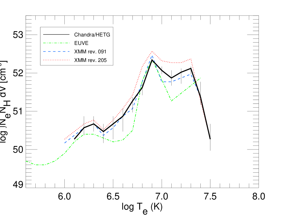
Figure 11: Comparison of EMDs derived from different instruments. The EMD from EUVE observations (Sanz-Forcada et al., 2002) was scaled for a coronal abundance of [Fe/H]=$-0.57$. Representative $1-\sigma$ error bars are shown for the Chandra/HETG EMD only (note that these error bars are not independent, see text).

The general shape of the EMD derived from XMM and Chandra is consistent with the EMD obtained with EUVE (Sanz-Forcada et al., 2002), indicating a corona dominated by multi-T plasma with a peak at log $T$(K)$\sim$6.9, very well constrained by the line fluxes (see Fig. 11). The EMD at higher temperatures is supported by a large number of lines from different elements identified in the HETG and RGS spectra. Finally a lower peak seems to be present around log $T$(K)$\sim$6.3. However, the lack of coverage of Fe lines makes the results for the EMD at log $T$(K)$\la$6.6 less robust than for higher temperatures.

Comparison of the EMDs reconstructed at different times (Fig. 11), including those of the XMM observations corresponding to different levels of activity of AB Dor, shows that the EMD peak is very stable, and thus an increase in the emission level is linked to higher emission measure values at all temperatures. The EMDs based on Chandra and XMM data show a steep increase with temperature in the range log $T$(K)$\sim$6.4–6.9, with a slope comprised between $T^{4}$ and $T^{5}$, while they are almost flat from the peak up to log $T$(K)$\sim$7.3.

Table 6: Abundances of the elements ([X/H], solar units)

X	FIP	HETG	HETG	XMM 091	XMM 091	XMM 205
	eV	(3-T)	(EMD)	(3-T)	(EMD)	(EMD)
Al	5.98	-0.62$\pm$0.33	-0.35$\pm$0.13	…	…	…
Ca	6.11	-0.90$\pm$0.59	0.23$\pm$0.63	-1.07$\pm$0.50	0.38$\pm$0.26	0.62$\pm$0.32
Ni	7.63	-0.87$\pm$0.18	-0.20$\pm$0.11	-0.41$\pm$0.10	-0.08$\pm$0.37	-0.28$\pm$0.29
Mg	7.64	-0.69$\pm$0.04	-0.39$\pm$0.12	-0.46$\pm$0.05	-0.43$\pm$0.17	-0.34$\pm$0.14
Fe	7.87	-0.85$\pm$0.03	-0.57$\pm$0.04	-0.67$\pm$0.02	-0.57$\pm$0.07	-0.57$\pm$0.07
Si	8.15	-0.60$\pm$0.04	-0.47$\pm$0.09	-0.40$\pm$0.08	-0.39$\pm$0.29	-0.37$\pm$0.17
S	10.36	-0.50$\pm$0.11	-0.20$\pm$0.16	-0.57$\pm$0.08	-0.32$\pm$0.22	-0.49$\pm$0.21
C	11.26	…	…	-0.36$\pm$0.04	-0.02$\pm$0.23	-0.05$\pm$0.16
O	13.61	-0.55$\pm$0.04	-0.15$\pm$0.11	-0.54$\pm$0.02	-0.05$\pm$0.11	-0.03$\pm$0.09
N	14.53	-0.40$\pm$0.22	-0.04$\pm$0.14	-0.28$\pm$0.05	0.20$\pm$0.13	0.10$\pm$0.11
Ar	15.76	-0.49$\pm$0.41	0.05$\pm$0.22	-0.42$\pm$0.16	-0.05$\pm$0.33	0.09$\pm$0.20
Ne	21.56	-0.21$\pm$0.03	0.13$\pm$0.10	-0.03$\pm$0.02	0.28$\pm$0.10	0.25$\pm$0.11

The electron densities calculated using the O vii triplet (log $n_{\rm e}$[cm^-3]$\sim$10.7–10.9 at log $T$[K]$\sim$6.3) are consistent in the three observations of HETG and RGS (Table 7). The value obtained for rev. #091 is also close to the one (log $n_{\rm e}$[cm^-3]$\sim$10.3${}^{+0.3}_{-0.4}$) reported by Güdel et al. (2001). The density calculated from the Ne ix triplet (log $n_{\rm e}$[cm^-3]$\sim$11 at log $T$[K]$\sim$6.6) is the value most affected by the presence of lines not deblended, and evaluated using the atomic model combined with the EMD (see also Brickhouse, 2001), and hence it has to be considered more uncertain. Higher densities (log $n_{\rm e}$[cm^-3]$\ga$12 at log $T$[K]$\sim$6.9) are indicated by the Mg xi triplet. Finally, the Fe xxi and Fe xxii densities (Table 8) are obtained from lines that are quite well measured, and with little contributions from blends. Values in the range log $n_{\rm e}$(cm^-3)$\sim$12.3–12.8 are indicated by most of these lines which form at $T\sim$10 MK, having excluded the two most discrepant values. The results clearly suggest an increase of the electron density with temperature, also observed for Capella (Brickhouse, 2001; Argiroffi et al., 2003), and formerly suggested by EUVE observations of Capella and other active stars (see Brickhouse, 1996; Drake, 1996; Sanz-Forcada et al., 2002, and references therein).

In particular, the results obtained with the Mg xi triplet and the Fe xxi and Fe xxii line ratios seem to confirm the findings already derived from EUVE (Dupree et al., 1993; Brickhouse, 1996; Sanz-Forcada et al., 2002, 2003a) and Chandra (Huenemoerder et al., 2001, 2003) data, with densities of at least log $n_{\rm e}$(cm^-3)$\sim$12 at log $T$(K)$\sim$6.8–7.1.

4.2 Element abundances

Coronal element abundances are subject of some controversy because of the different results (in many cases contradictory) found in the comparison from observations with different instruments and/or analyzed with different techniques (see Favata & Micela, 2003, and references therein). Stars with low levels of activity tend to show similar trends with the First Ionization Potential (FIP) as in the solar case (see Bowyer et al., 2000, and references therein), with elements with low FIP ($<$10 eV; e.g. Mg, Si, Fe) being enhanced with respect to elements with higher FIP ($\geq$ 10 eV; e.g. O, Ne, Ar) when compared with the photospheric values. The opposite effect is observed instead for more active stars (the so called MAD —“Metal abundances deficient”— effect, or the “inverse FIP effect” Schmitt et al., 1996; Brinkman et al., 2001; Drake et al., 2001). However, many of the studied active stars lack accurate information on the photospheric abundances, and/or show contradictory results depending on the technique applied in the analysis. We have carried out the two most typical approaches for the coronal analysis (global-fitting to the spectrum and EMD reconstruction from line fluxes) in order to clarify what is the origin of this discrepancy. The use of the EMD reconstruction approach shows very consistent results (see Table 6 and Fig. 12) for the different instruments, while the global-fitting results are not convergent, and show contradictory results (e.g. for Ni, Mg, Fe or Ne, see Table 6) in HETG and RGS for observations with similar flux level. The line-based analysis applied to Chandra and XMM data show a clear and consistent pattern of the abundances vs. FIP. An initial depletion of the abundances seems to be present for elements with FIP increasing up to the Fe value, and a progressive increment of the abundances for the elements with higher FIP (a similar behavior seems to be present in the case of AR Lac, Huenemoerder et al., 2003). Photospheric abundances of AB Dor are near solar photospheric values (with [Fe/H]$\sim$0.1 Vilhu et al., 1987). Coronal Fe abundance depletion for AB Dor was already found from EUVE and ASCA observations (Rucinski et al., 1995; Mewe et al., 1996), now confirmed by the HETG and RGS analysis.

The EMD can be extended down to log $T$(K)$\sim$4 through the measurements of lines in the UV. Sanz-Forcada et al. (2002) reported measurements from IUE not simultaneous to those of EUVE, and constructed an EMD of AB Dor in the range log $T$(K)$\sim$4.0–7.3. The calculation of the EMD in the lower temperature region (approximately log $T$[K]$\sim$4.0–5.5) was dominated basically by C lines, while the determination of the EMD for log $T$(K)$\ga$5.6 depends on Fe lines only. The combined data of IUE and EUV, in absence of better information, indicated a minimum of the EMD around log $T$(K)$\sim$5.8. The calculation of the [C/Fe] abundance with RGS allows us to correct the position of this minimum. Assuming that the value of [C/Fe]$\sim$0.5 is constant in the whole range of temperature, and the general flux levels of these observations is similar, the EMD calculated in the corona by (Sanz-Forcada et al., 2002) should be 0.5 dex higher, and the minimum of the EMD should occur at a lower temperature, log $T$(K)$\sim$5.3. Measurements of lines formed in the region log $T$(K)$\sim$5–6 would be needed in order to nail the temperature of this minimum.

Figure 9: Electron densities from He-like triplets (see Table 7).

5 Discussion and conclusions

Our analysis of the Chandra/HETG and XMM/RGS spectra has provided consistent results in terms of the plasma emission measure distribution (EMD) vs. temperature, the abundances of individual elements in corona, and even the plasma density as determined from the O vii He-like triplet. The superior spectral resolution of the Chandra instrument has also allowed us to obtain reliable estimates of the plasma density at different temperatures using the Ne ix and Mg xi triplets, as well as density-sensitive Fe xxi and Fe xxii line ratios. The corona of AB Dor appears to have a quite stable thermal structure with an amount of plasma steeply increasing with temperature from log $T$(K)$\sim 6.4$, to log $T$(K)$\sim 6.9$. A substantial amount of plasma (within a factor 2 from the peak value) is also present in a plateau of the EMD extending up to $T\sim 2\times 10^{7}$ K. A less constrained secondary peak is possibly also present at $T\sim 2\times 10^{6}$ K, the characteristic temperature of the corona of the quiet Sun.

The above description applies to AB Dor in quiescent state, i.e. outside of any evident isolated flaring event, and it is essentially in agreement with the information already available from previous observations of AB Dor with EUVE. However, the quiescent X-ray emission is not steady, but characterized by significant variability on time scales shorter than the rotation period, suggestive of a very dynamic corona where a large number of small-scale flares may occur at any time. On the other hand, we recall that AB Dor is also capable of producing very strong flares, which may affect the coronal thermal structure quite significantly: in the extreme case of the flares observed by SAX (Maggio et al., 2000), the peak value of the total volume emission measure was of the order of $10^{54}$ cm^-3 at a temperature $T\sim 10^{8}$ K.

Figure 10: Electron densities from Fe xxi (dashed lines) and Fe xxii (solid lines) lines ratios, as indicated in Table 8.

By comparing the EMDs corresponding to the lowest and highest X-ray emission levels observed in the first three years of XMM-Newton observations we learn that an increase of the source luminosity (in the range 6–20 Å) from $L_{\rm x}=6.8\times 10^{29}$ erg s^-1 (Jun 2000) to $L_{\rm x}=1.2\times 10^{30}$ erg s^-1 (Jan 2001), not associated to any large flare, can be explained by an increase of the whole EMD by factors 1.2–3, with the largest variation occurring in the level of the high-temperature plateau of the EMD. In principle, larger emission measures can be obtained with a (linear) increase of the emitting volume, or a (square root) increase of the plasma density, or both. Unfortunately, the statistical uncertainties on the density derived from the analysis of the O vii triplet at the two epochs does not allow us to distinguish between these possibilities.

Plasma densities are a key parameter to try to interpret the above scenario in terms of classes of magnetically-confined coronal structures. The measurements of the O vii triplet (log $n_{\rm e}$[cm^-3]$\sim$10.8) yield plasma pressures $p_{\rm e}\sim 20-40$ dyn cm^-2 at $T\sim 1$–$2\times 10^{6}$ K, already quite high for solar standards. Even higher values are indicated by a number of other line ratio diagnostics derived from the Chandra/HETG data only. In particular, the Ne ix triplet (log $n_{\rm e}$[cm^-3]$\sim$11) indicates a pressure $p_{\rm e}\sim 10^{2}$ dyn cm^-2 at $T\sim 3$–$5\times 10^{6}$ K, while the Mg xi triplet (log $n_{\rm e}$[cm^-3]$\sim$12.4) and the density-sensitive Fe xxi and Fe xxii lines (log $n_{\rm e}$[cm^-3]$\sim$12.5) suggest a pressure increasing from $p_{\rm e}\sim 2\times 10^{3}$ dyn cm^-2 up to $\sim 0.7$–$2\times 10^{4}$ dyn cm^-2 for plasma temperatures in the range $5\times 10^{6}$–$2\times 10^{7}$ K.

Taking into account also the results obtained by Schmitt et al. (1998) and by Ake et al. (2000) from C iii line ratios – log $n_{\rm e}$(cm^-3)$\sim$11, yielding $p_{\rm e}\sim 2.2$ dyn cm^-2 at $T\sim 8\times 10^{4}$ K, i.e. at the base of the transition region – we derive the picture illustrated in Fig. 13: the plasma pressure appears to increase steadily from the transition region to the corona, with a steeper and steeper piece-wise power-law dependence on temperature (from $T^{0.7}$ at low temperatures, up to $T^{5}$ in the range of the EMD plateau). Note that this relationship was found using the peak temperatures of the line emissivity functions weighted by the EMD; a slightly different but qualitatively consistent behavior would appear considering the effective temperatures of line formation provided by the $(f+i)/r$ ratios, available for the He-like triplets only.

Table 7: Electron densities calculated from He-like triplets

Ion	($f+i$)/$r$	$T_{\rm ratio}$	$f$/$i$	log $n_{\rm e}$(cm-3)	Instrument
O vii	0.83$\pm$0.06	6.24$\pm$0.07	1.44$\pm$0.17	10.77$\pm 0.08$	RGS (091)
O vii	0.78$\pm$0.05	6.33$\pm$0.06	1.36$\pm$0.13	10.82$\pm 0.06$	RGS (205)
O vii	0.86$\pm$0.15	6.2$\pm$0.2	1.4$\pm$0.3	10.78$\pm$0.14	HETG
Ne ix	0.67$\pm$0.04	6.6$\pm$0.1	2.9$\pm$0.3	10.95${}^{+0.2}_{-0.5}$	HETG
Mg xi	0.75$\pm$0.08	6.7$\pm$0.1	2.2$\pm$0.3	12.4${}^{+0.2}_{-0.3}$	HETG
Si xiii	0.66$\pm$0.05	6.7$\pm$0.1	3.9$\pm$0.5	$\la$11.5	HETG

Table 8: Electron densities calculated from Fe xxi and Fe xxii line ratios.

No.a	Ion	Lines ratio	$T_{\rm max}$	log $n_{\rm e}$(cm-3)
1	Fe xxi	$\lambda$12.284/$\lambda$12.499	7.0	12.80$\pm 0.13$
5	Fe xxi	$\lambda$12.393/$\lambda$12.499	7.0	12.29$\pm 0.14$
2	Fe xxii	$\lambda$11.770/$\lambda$11.932	7.1	13.22$\pm 0.12$
3	Fe xxii	$\lambda$11.932/$\lambda$8.9748	7.1	12.0${}^{+0.2}_{-0.5}$
4	Fe xxii	$\lambda$11.932/$\lambda$11.802	7.1	12.4${}^{+0.2}_{-0.3}$
6	Fe xxii	$\lambda$11.490/$\lambda$11.932	7.1	12.74$\pm 0.14$
7	Fe xxii	$\lambda$12.210/$\lambda$11.932	7.1	12.79$\pm 0.12$

($a$): Number corresponding to labels in Fig. 10

The steep increase of the plasma pressure with temperature is possibly one of the most intriguing results provided by the currently available Chandra high-resolution spectra of active stars (Favata & Micela, 2003). A similar trend was recently found in Capella by Argiroffi et al. (2003), and tentatively interpreted as due to the presence of different classes of coronal loop structures in isobaric conditions, having increasing pressures but decreasing volume filling factors for increasing maximum temperature of the trapped plasma.

The effective scale sizes and volumes of the structures responsible for the X-ray emission from stellar coronae essentially depend on two parameters: the plasma pressure scale height and the strength of the magnetic field required for plasma confinement. In the case of AB Dor, having a stellar radius $R_{*}\sim 1$ R_☉ and a surface gravity $g\sim 0.8$ g_☉ (Maggio et al., 2000), we get pressure scale heights $H_{\rm p}\sim 1.5\times 10^{10}$ cm ($0.2R_{*}$) for coronal loops with maximum temperature $T_{\rm max}=2\times 10^{6}$ K, and $H_{\rm p}>7.5\times 10^{10}$ cm ($>1.1R_{*}$) for the structures having $T_{\rm max}=10^{7}$ K or hotter, which represent the dominant class in the corona of AB Dor. If the ratio between the plasma pressure and the magnetic field pressure, $\beta$, is larger than unity at the maximum height, $L\leq H_{\rm p}$, above surface dictated by the pressure scale height, then magnetic confinement is effective at these heights and the volume of the emitting plasma in the visible stellar hemisphere can be expressed as

$$V_{\rm max}\approx 2\pi fR_{*}^{2}L$$ (2)

where $f$ is a surface filling factor. The minimum field required to confine the plasma at a height $L$ is given by

$$B_{\rm min}(L)=(8\pi p_{\rm e})^{1/2}$$ (3)

From the available data we derive $B_{\rm min}\sim 30$ G at $T\sim 2\times 10^{6}$ K ($p_{\rm e}=35$ dyn cm^-2) and $B_{\rm min}\sim 460$ G at $T\sim 10^{7}$ K ($p_{\rm e}=8.5\times 10^{3}$ dyn cm^-2). Donati & Collier Cameron (1997) found that up to 20% of the surface of AB Dor is covered with magnetic regions having typical values of 500 G and peaks of 1.5 kG. Assuming that magnetic field at the stellar surface is 1.5 kG and that the field strength decreases with height as in a magnetic dipole ($B\sim r^{-3}$) rooted at the base of the convection zone (so from $r\sim 0.5R_{*}$ to $r\sim 0.5R_{*}+L$), we estimate that the plasma at $2\times 10^{6}$ K can be confined up to heights $L=9.4\times 10^{10}$ cm ($1.3R_{*}$), while in the worst case of the high temperature ($10^{7}$ K) coronal structures, the maximum height is $L=1.7\times 10^{10}$ cm ($0.24R_{*}$). Since the characteristic height of the high temperature structures is smaller than $H_{\rm p}$, the isobaricity of the plasma is ensured. We can estimate the filling factor $f$ by equating $n_{\rm e}^{2}V_{\rm max}=EM$, where $n_{\rm e}$ and $EM$ are the plasma density and volume emission measure derived from our analysis. In this way we derive $f\sim 2\times 10^{-6}$ at $T\sim 10^{7}$ K. In the case of the low-temperature plasma, the observed emission originates mostly from the plasma below the pressure scale height $H_{\rm p}$, and the effective filling factor can be derived by replacing $L$ with $H_{\rm p}$, resulting in $f\sim 2\times 10^{-4}$ at $T\sim 2\times 10^{6}$ K. These filling factors can be usefully compared with the $\sim 7$% fraction of surface in the polar cap of AB Dor above $60^{\degr}$ latitude: this is a region always in view as the star rotates, where high field strengths are suggested by Zeeman-Doppler images (Jardine et al., 2002) and where a non-potential field component (i.e. capable of providing free energy to power flares) is possibly present (Hussain et al., 2002). Larger filling factors are possible if the loops are significantly shorter than the stellar radius.

Figure 12: Element abundances in the corona of AB Dor, with respect to solar photosphere. A dashed line indicates the solar photospheric abundance (Anders & Grevesse, 1989).

A more refined model of the size, strength and orientation of the magnetic regions is however required to constrain better the possible sizes and locations of the X-ray emitting regions in the corona of AB Dor, as suggested by the simulations performed by Jardine et al. (2002). These authors have modeled the AB Dor coronal X-ray emission by extrapolating the magnetic field from the stellar surface to the corona using as a basis Zeeman-Doppler maps and assuming the field to be potential and the trapped plasma in hydrostatic equilibrium. However, their results rely on the further assumption of an isothermal plasma, which is clearly recognized as a too simplistic approximation. Based on the above model, Jardine et al. conclude that in most of the cases they have explored, the coronal emission of AB Dor should exhibit little rotational modulation: in fact, assuming low plasma densities, the corona turns out to be very extended (in order to account for the observed total volume emission measure) and hence the X-ray emission is little affected by the stellar rotation, while in the high-density case the emitting corona is more compact, but the X-ray brightest regions are at high latitudes and always visible as the star rotates. Exception to this behavior is predicted by models having high-temperature ($T=10^{7}$ K) plasma with densities in excess of $10^{12}$ cm^-3, i.e. with exactly the characteristics of the plasma near the peak of the emission measure distribution, as derived in this work. The occurrence and amplitude of the rotational modulation of the X-ray emission from this hot plasma is an issue that we intend to explore in the next step of our ongoing investigation.

The corona of AB Dor, even outside strong isolated flares, appears quite variable on time scales shorter than the rotation period. The only possible analogy with the case of the solar corona if a behavior where small-scale flares are continuously occurring in what can be defined a non-steady quiescent X-ray emission state. However, the stability found in the peak of the EMD at log $T$(K)$\sim$6.9 suggests coronal structures in stationary condition, and a simple increase in the number of loops having maximum temperatures in the range spanned by the EMD plateau may explain the variations of the EMD observed at the times of the lowest and highest emission level observed up to now by XMM.

Figure 13: Electron pressure derived from the electron densities at different temperatures (see text). Last two points represent averages over different density values in Table 8.

In conclusion, we summarize the main results of the present work as follows:

– The Emission Measure Distribution (EMD) has been calculated for the plasma of AB Dor by measuring the line fluxes in XMM/RGS and Chandra/HETG spectra, showing consistent results. The EMD is described by a quite stable structure, with a steep increase ($EM[T]\propto T^{\alpha}$, with $\alpha=$ 4–5) up to the peak at log(T)=6.9, followed by a plateau in the range log(T)=6.9–7.3. The EMD during the highest and lowest X-ray emission levels shows an increment in the amount of material that is rather uniform at all temperatures.

– Element abundances in the corona of AB Dor follow an intermediate behavior between the solar-like FIP (First Ionization Potential) effect, and the so called “inverse FIP effect” observed in other active stars.

– High electron densities were measured using He-like triplets and Fe xxi and Fe xxii line ratios. Together with the volume emission measure they allow to put constrains on the surface filling factor of the emitting regions and on the strength of magnetic fields required for plasma confinement.

– The available data are consistent with a scenario of a corona composed by several families of loops, shorter than but comparable to the stellar radius and in isobaric conditions, having plasma pressures increasing with the maximum plasma temperature; the surface filling factors of these structures is small. These structures can be easily accommodated in the stellar polar cap, where strong magnetic fields possibly in a non-potential state have been proposed. Larger filling factors are possible if the loops are significantly shorter than the stellar radius.