First Microlensing Candidates From The MEGA Survey Of M31

We present the first M31 candidate microlensing events from the Microlensing Exploration of the Galaxy and Andromeda (MEGA) survey. MEGA uses several telescopes to detect microlensing towards the nearby Andromeda galaxy, M31, in order to establish whether massive compact objects are a significant contribution to the mass budget of the dark halo of M31. The results presented here are based on observations with the Isaac Newton Telescope on La Palma, during the 1999/00 and 2000/01 observing seasons. In this data set, 14 variable sources consistent with microlensing have been detected, 12 of which are new and 2 have been reported previously by the POINT-AGAPE group. A preliminary analysis of the spatial and timescale distributions of the candidate events support their microlensing nature. We compare the spatial distributions of the candidate events and of long-period variable stars, assuming the chances of finding a long-period variable and a microlensing event are comparable. The spatial distribution of our candidate microlensing events is more far/near side asymmetric than expected from the detected long-period variable distribution. The current analysis is preliminary and the asymmetry not highly significant, but the spatial distribution of candidate microlenses is suggestive of the presence of a microlensing halo.

1 Introduction

One of the astrophysical solutions to the galactic dark matter problem would be the presence of a significant amount of undetected compact objects in the halos of galaxies. These MACHOs (Massive Astrophysical Compact Halo Objects) can be detected using gravitational microlensing (Paczynski Pacz86 (1986)). According to gravitational lensing theory the measured brightness of a background source will temporarily increase if a massive compact object moves close enough through our line of sight towards the background source.

During the last decade, the MACHO (Alcock et al. Alcock93 (1993)) and EROS (Aubourg et al. Aubourg93 (1993)) collaborations have been monitoring fields in the Large and Small Magellanic Clouds (LMC and SMC) in order to detect such events. After 5.7 years of observing the MACHO group found 13-17 microlensing events towards the LMC, and concluded that up to 20% of the Milky Way dark halo may consist of compact objects of mass 0.15 - 0.9 $M_{\odot}$ (Alcock et al. Alcock00 (2000)). The EROS collaboration has found 3 microlensing events towards the LMC and puts strong constraints on the fraction of dark matter in the form of compact objects (Lasserre et al. Lasserre00 (2000)). The results of both groups are, however, consistent with $\sim$10% of the dark halo mass consisting of compact objects of $\sim$0.5$M_{\odot}$ (e.g. Milsztajn Milsztajn02 (2002)).

Looking for microlensing events in the nearby Andromeda galaxy (M31) has several advantages over Magellanic Clouds searches (Crotts Crotts92 (1992); Baillon et al. Baillon93 (1993)). Because of the geometry the microlensing optical depth can be up to ten times larger in parts of M31. In combination with the extremely high density of background stars, this results in a highly enhanced microlensing rate. Due to the high inclination of the disk of M31, it should be possible to use microlensing to constrain the mass contribution of compact objects to the dark halo (Baltz, Gyuk & Crotts Baltz03 (2003); Gyuk & Crotts GyukCrotts00 (2000); Kerins et al. Kerins01 (2001)). In the presence of a significant microlensing halo, the microlensing rate should be asymmetric, with more microlensing taking place towards the far side of the disk than to the near side, because the line-of-sight through the halo is longer towards the far side.

Besides these advantages, M31 microlensing also has some problems. Because of the large distance the stars are faint and generally unresolved from the ground. However, using special techniques, it is possible to detect microlensing in M31 (e.g. Crotts & Tomaney CrottsTomaney96 (1996); Paulin-Henriksson et al. Paulin03 (2003); Calchi Novati et al. Calchi03 (2003)). Three collaborations are currently working on microlensing surveys in M31, namely POINT-AGAPE (Aurière et al. Auriere01 (2001)), WeCAPP (Riffeser et al. Riffeser01 (2001)) and MEGA (Crotts et al. MEGA (2001)).

The Microlensing Exploration of the Galaxy and Andromeda (MEGA) collaboration has performed an intensive four-year survey of two large fields in M31 plus extended baseline observations in order to measure the microlensing optical depth due to a possible MACHO halo. In this paper we present the first microlensing candidates resulting from the analysis of the 1999-2000 and 2000-2001 season data obtained at the Isaac Newton Telescope at La Palma. In section 2 we briefly describe the dataset and methods used. The microlensing candidates are presented in section 3. Our discussion and conclusions are presented in section 4. Finally, future work is outlined in section 5.

2 Data and Method

2.1 Dataset

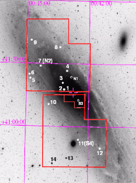
MEGA uses several telescopes to monitor two wide fields, covering a total area of 0.57 square degrees. For the current analysis, observations done with the Wide Field Camera (WFC) on the Isaac Newton Telescope (INT) were used. The layout of the WFC chips on M31 is shown in Figure 1. We present microlensing events from the 1999/2000 and 2000/2001 observing seasons. The observations in the first season (99/00) were spread over 57 nights between August 1st 1999 and January 4th 2000 and were taken in the Sloan r^′, g^′ and i^′ broad bands. The r^′ dataset is the largest with 57 epochs, whilst the g^′ and i^′ datasets contain 41 and 24 epochs respectively. During the second observing season (00/01) 90 epochs were obtained in both r^′ and i^′, between August 1st 2000 and January 23 2001. Observations were spread equally over both fields. The exposure time per epoch ranges between 5 and 30 minutes and is typically 10 minutes. Because the WFC is not always mounted on the INT, the epochs tend to cluster in blocks of two to three weeks. Part of the data from the 2001/2002 season has been used as well. From this third season, 19 epochs in r^′ and i^′ taken between August 13th 2001 and November 18th 2001 were used to extend the baselines of the events from the first two seasons in order to exclude long period variable stars. These data were not used to detect more microlensing events.

Figure 1: The layout of the two INT Wide Field Camera (WFC) fields in M31 used for the microlensing search described in this paper. The WFC has four 2048x4100 pixel chips with a pixel scale of 0.333″, offering a field of view of approximately 0.25$\Box^{o}$. With this field layout we cover a large part of the far side (SE) of the disk of M31 as well as part of the near side. Also plotted are the positions of the candidate microlensing events in our sample (full circles). Note that our events 7 and 11 correspond to the events PA-99-N2 and PA-00-S4 reported previously by POINT-AGAPE. Part of the south field close to the bulge is not used for our analysis, since the image subtraction is not of high quality in this very high surface brightness area. This region is indicated in the uppermost chip of the south field. The two POINT-AGAPE events not present in our sample are indicated with the open circles.

2.2 Data reduction

Standard data reduction, including bias subtraction, trimming and flatfielding was performed in IRAF. Because of the high stellar density in M31 and its large distance, the background source stars are usually resolved only while they are being lensed and sufficiently magnified. To detect microlensing events in these fields, we use the Difference Image Photometry (DIP) method as described by Tomaney & Crotts (TomaneyCrotts96 (1996)). This method involves subtracting individual images from a high quality reference image, resulting in difference images in which variable objects show up as residuals.

Below we outline the steps of the DIP pipeline that was used. All operations are done in IRAF, using the DIFIMPHOT package written primarily by Austin Tomaney, unless explicitly stated otherwise.
$\bullet$ Astrometric registration and stacking of images
All images are transformed to a common astrometric reference frame. By stacking high quality images from the 1999 season, a high signal-to-noise reference image was made. Per night all exposures are combined separately for each band. Each epoch corresponds to the combination of all frames taken in the same band in one night. The Julian date of the epoch is taken as the weighted average of the Julian dates of the individual frames.
$\bullet$ Image subtraction
From the single epoch images the high signal-to-noise reference image is subtracted, after photometric calibration and matching of the point spread function (PSF) between the images (Tomaney & Crotts TomaneyCrotts96 (1996)). The shape of the PSF is measured from bright, unsaturated stars in the images that are being matched. By dividing the PSFs in Fourier space a convolution kernel is calculated with which the better seeing image (usually the reference image) is degraded.
$\bullet$ Variable object detection
The resulting difference images are dominated by shot noise in which variable sources show up as positive or negative residuals, depending on the flux difference of the object between the single epoch image and the reference image. Due to fringing, the i^′ difference images are of poorer quality than the r^′ difference images. SExtractor (Bertin & Arnouts SExtractor (1996)) is used to detect residuals in all r^′ difference images from the first two observing seasons. The catalogs with residuals are cross-correlated to obtain a catalog with all variable objects in the surveyed fields. As a first selection to get rid of noisy detections, we demand that objects have to be detected in at least two epochs.
$\bullet$ Lightcurves and Epoch quality
Lightcurves for the variable sources are obtained by performing PSF fitting photometry on the residuals in the difference images, using the PSF shape measured from the bright unsaturated stars. Several epochs turned out to give problematic difference images for a number of different reasons. Epochs with seeing worse than 2.0″ do not give clean difference images and were discarded. A small number of epochs were overexposed and had to be discarded as well.
Lightcurves were also produced at “empty” positions, i.e. positions were no variability was detected. Flat line fits were done to these empty lightcurves to check the error bars on the fluxes derived from statistics of the PSF fitting photometry. For each epoch, the distribution of the deviations from the flat lightcurve fits weighted by the error bar returned by the photometry routine was examined. In some cases this distribution showed broad non-gaussian wings, and these epochs were discarded. Typically they were associated with highly variable seeing between the individual exposures. In other cases, the normalized error distribution was gaussian, but with dispersion higher than one. In these cases the error bars were renormalized appropriately.

The typical number of epochs that were left after the procedure described above are tabulated in table 1 for each filter and field for the 99/00 and 00/01 seasons. From these epochs the lightcurves were constructed that were used for the analysis presented in this paper.

	r′		i′
	F1	F2	F1	F2
99/00	46	45	16	15
00/01	56	55	56	56
Total	102	100	72	71

Table 1: Overview of the number of epochs used for seasons 1 and 2, field and filter. F1 is the north field and F2 is the south field.

2.3 Event selection

The final dataset consists of lightcurves of 118,424 variable sources, practically all of which are periodic variable stars. Finding candidate microlensing events in such a large number of lightcurves is no trivial problem. A procedure to select lightcurves that are compatible with microlensing must be aimed at recognizing the characteristics of a microlensing lightcurve while taking into account computing speed, and the quality of the available data. Since the quality of the i^′ band data was clearly poorer than the quality of the other bands, and since g^′ data were only available for the first season, we decided to use the r^′ data as the main basis for candidate selection. Another advantage of the r^′ data is that they have much better sampling density in the first season than do i^′ and g^′ data separately. Thus, the first steps of the filtering process involved only r^′ data, after which the i^′ data are used to further analyse the r^′ microlensing candidates.

A microlensing event caused by a single lens has a characteristic shape and a flat baseline. The selection steps based purely on the r^′ lightcurves are aimed at selecting lightcurves with flat baselines and well sampled, significant peaks which fit the characteristic microlensing shape well. A detailed description of these steps is given in Appendix A1. To make sure these selection steps do a good job selecting microlensing events and rejecting long-period variable stars, Monte Carlo simulations of microlensing events and long-period variables were performed and used to fine tune the selection procedure. Based on just the r^′ data we select 1,347 lightcurves.

Colour information can be used for the microlensing candidate selection for several reasons. Contrary to variable stars, microlensing events are intrinsically achromatic, meaning that the colour of the observed difference flux remains the same during the event. Furthermore, long-period variable stars that might be mistaken for microlensing are very red. Because of this, the brightness variations are also more pronounced in i^′ than in r^′. Further selection steps, described in more detail in Appendix A2, include a colour cut designed to reject long-period variables and a goodness of fit criterion for the i^′ lightcurve. For the latter, the i^′ lightcurves are fit with a standard microlensing lightcurve with the shape parameters found for the r^′ lightcurves, as a test for achromaticity.

Figure 2: Lightcurves of the 14 microlensing candidate events. This page shows candidates 1 through 5, with the r^′ lightcurves plotted in the upper panel and the i^′ lightcurves in the lower panel. The Julian Date of the zeropoint of the time axis is 2451393, which corresponds to August 1st 1999.

Figure 2: continued – Candidates 6 through 10.

Figure 2: continued – Candidates 11 through 14.

This complete automated selection procedure results in 126 candidate microlensing events from the 99/00 and 00/01 observing seasons. Unfortunately, rather lenient $\chi^{2}$ cuts had to be used for the goodness of fit criteria. This is due to the photometry being too sensitive to nearby variable sources, as described in more detail in Appendix A. Because of this, the sample still contains lightcurves with slightly variable baselines. The lightcurves and the difference image residuals of these candidate events had to be inspected visually to establish whether any additional variability was intrinsic to the variable source or was caused by nearby sources. An effort to improve the photometry in the presence of neighbours is underway. The lightcurves with baseline variability that could not be attributed to nearby variable sources, in total 67, were thrown out. In a further 39 cases, the detected candidate event was actually caused by bad pixels and these were discarded as well, so after visual inspection, 21 events remain that are consistent with microlensing based on the 2 year lightcurves. Finally, part of the data from the third (01/02) season were used to extend the baselines of these 21 events, 7 of which showed variability in the third season. The final set of candidate microlensing events consists therefore of the 14 events described in the following section.

3 Results

Candidate	RA	DEC	$t_{max}$	$t_{FWHM}$	$\Delta$r′	r′-i′
event	(J2000)	(J2000)	(days)	(days)	(mag)	(mag)
MEGA-ML 1	0:43:10.54	41:17:47.8	60.1 $\pm$ 0.1	4.2 $\pm$ 4.3	22.2 $\pm$ 1.1	1.1 $\pm$ 1.5
MEGA-ML 2	0:43:11.95	41:17:43.6	34.08 $\pm$ 0.08	4.6 $\pm$ 0.6	21.6 $\pm$ 0.3
MEGA-ML 3	0:43:15.76	41:20:52.2	420.06 $\pm$ 0.05	2.6 $\pm$ 2.2	21.8 $\pm$ 1.2	0.4 $\pm$ 1.5
MEGA-ML 4	0:43:04.08	41:26:15.6	429.7 $\pm$ 0.2	29.1 $\pm$ 1.0	22.8 $\pm$ 0.2	0.8 $\pm$ 0.3
MEGA-ML 5	0:44:48.95	41:22:59.3	398.1 $\pm$ 0.2	9.4 $\pm$ 4.1	22.9 $\pm$ 0.8	0.4 $\pm$ 1.0
MEGA-ML 6	0:44:50.97	41:24:42.4	77.3 $\pm$ 0.2	22.9 $\pm$ 0.7	22.6 $\pm$ 0.2
MEGA-ML 7	0:44:20.89	41:28:44.6	71.20 $\pm$ 0.06	21.6 $\pm$ 0.7	19.3 $\pm$ 0.2	1.4 $\pm$ 0.2
MEGA-ML 8	0:43:24.53	41:37:50.4	63.1 $\pm$ 0.2	27.4 $\pm$ 0.9	22.7 $\pm$ 0.2	0.8 $\pm$ 0.2
MEGA-ML 9	0:44:46.80	41:41:06.7	392.3 $\pm$ 0.2	3.8 $\pm$ 1.6	21.8 $\pm$ 0.8	0.4 $\pm$ 1.0
MEGA-ML 10	0:43:54.87	41:10:33.3	74.7 $\pm$ 0.4	46.8 $\pm$ 4.4	22.2 $\pm$ 0.3	1.0 $\pm$ 0.3
MEGA-ML 11	0:42:29.90	40:53:45.6	488.6 $\pm$ 0.05	2.0 $\pm$ 0.3	20.5 $\pm$ 0.2	0.3 $\pm$ 0.2
MEGA-ML 12	0:41:26.90	40:49:42.1	436.6 $\pm$ 0.6	131.0 $\pm$ 9.4	23.2 $\pm$ 0.3	1.0 $\pm$ 0.3
MEGA-ML 13	0:43:02.49	40:45:09.2	37.3 $\pm$ 0.5	22.8 $\pm$ 3.8	23.3 $\pm$ 0.3	0.5 $\pm$ 0.4
MEGA-ML 14	0:43:42.53	40:42:33.9	455.1 $\pm$ 0.3	28.1 $\pm$ 1.4	22.5 $\pm$ 0.2	0.3 $\pm$ 0.4

Table 2: Fit parameters for the 14 candidate microlensing events. The $t_{max}$ and $t_{FWHM}$ values are based on full parameter fits to the r^′ lightcurves. Also listed are the magnitude of the difference flux at maximum amplification and the r^′-i^′ colours where possible. For the short events, i.e. $t_{FWHM}$ in the order of a few days, the uncertainties are large, because the time sampling of the data is relatively sparse compared to the width of the peak. Peak times are in days after August 1st 1999.

Figure 3: Data points from the baseline of event 10, but now the $\Delta Flux$ is plotted as function of the seeing. During the period from which these points are taken, a variable source located about 7 pixels away from the event caused a strong residual in the difference images. There clearly is a trend with worse seeing corresponding to lower fluxes.

Figure 4: Thumbnails of three events, chosen to span a wide range of peak fluxes. The uppermost panel shows event 7, by far the brightest event, going down in flux through event 11 (middle panel) to the low signal-to-noise event 5 (lower panel). For each event we show thumbnails of the difference images and single epoch images in both r^′ and in i^′. Thumbnails were chosen from three epochs during the microlensing event, i.e. in the peak of the lightcurve, and from one epoch before and one epoch after the event. Event 7 (upper panel) stands out very clearly in both the difference images and the single epoch images in both bands. In the i^′ thumbnails a variable star is clearly visible in the lower left corner. The event in the middle panel, event 11, has a peak flux only one third of the peak flux of event 7, but still stands out clearly in the difference images. In the single epoch images, the event is only visible during maximum amplification. Event 5, shown in the lower panel is an example of the fainter events, with a peak flux almost an order of magnitude smaller than event 11. As can also be seen from the lightcurves (figure 2), the event is much brighter in r^′ than in i^′. In the r^′ difference images the residual is more obvious than in the i^′ difference images. The nearby variable source that influences the i^′ photometry is clearly visible just above and to the left of the event. In the single epoch images, the event is hardly visible at all without difference image techniques.

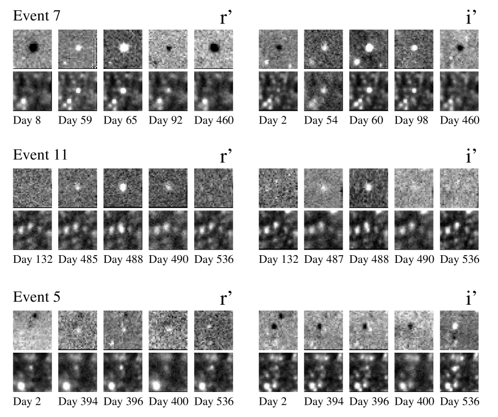
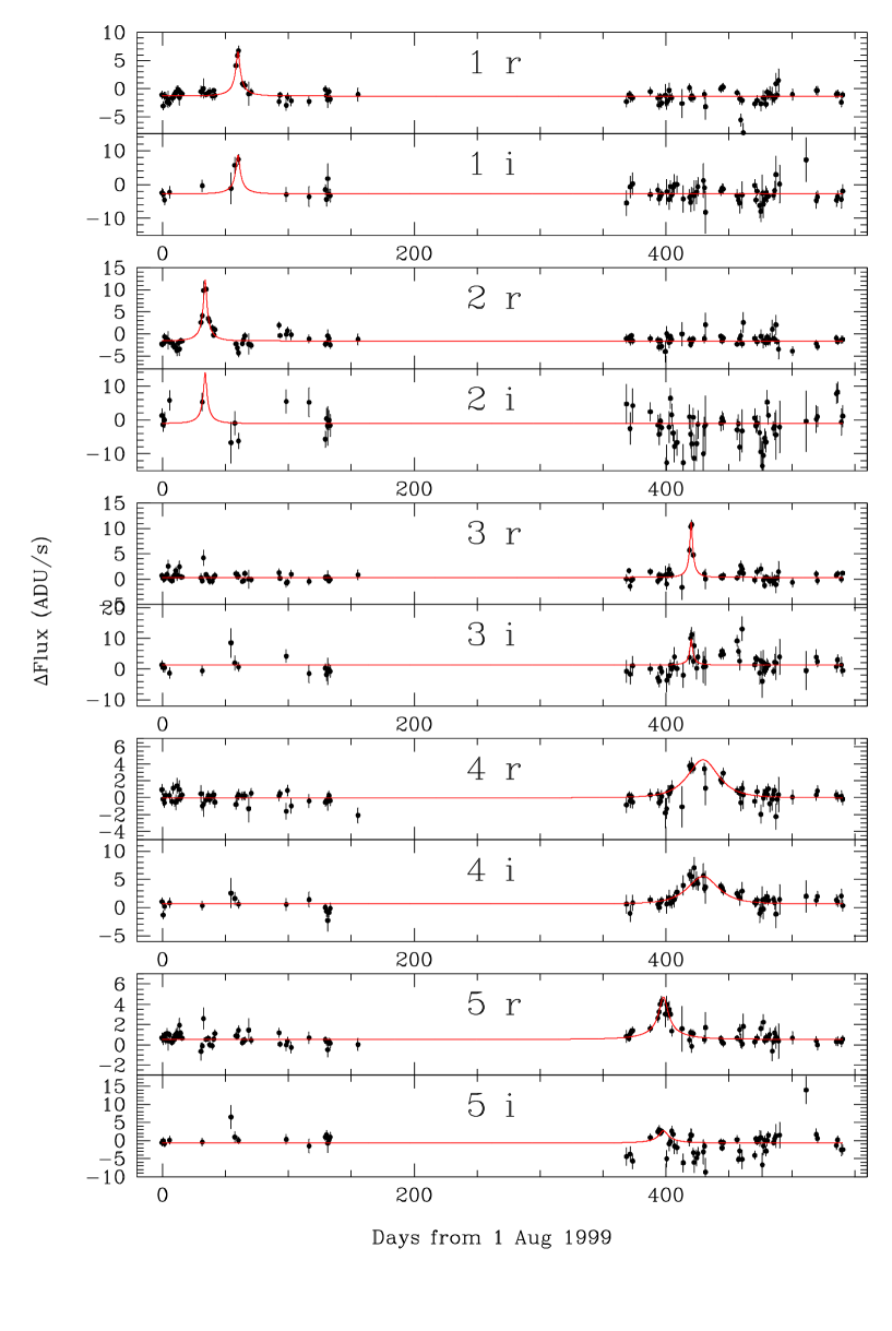
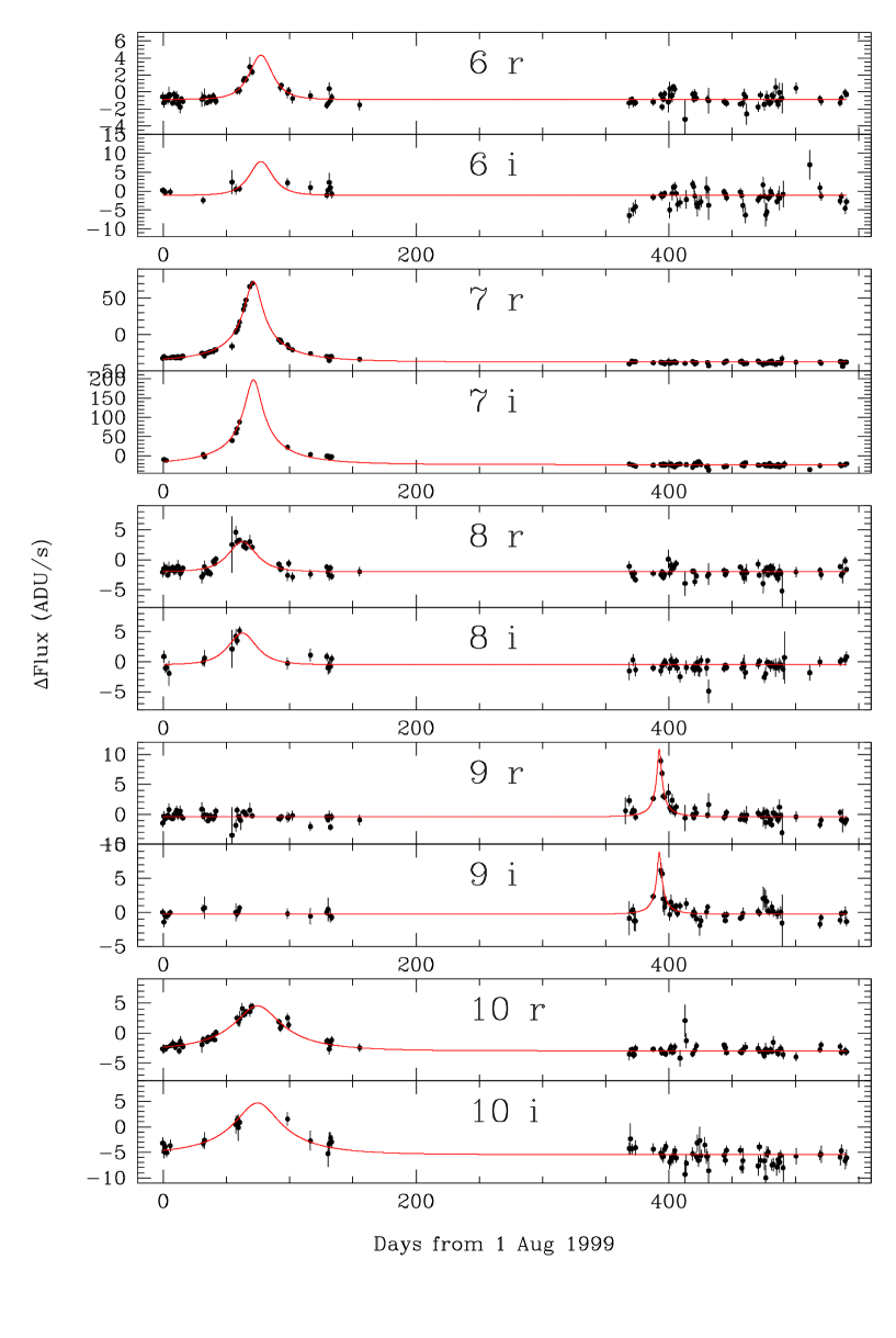
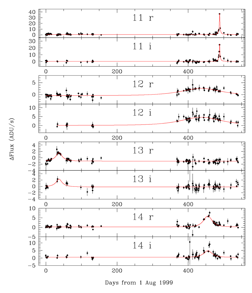
The lightcurves of the 14 candidate microlensing events are shown in figure 2; their positions are plotted in figure 1. August 1st 1999 was taken as the zero point of the time scale in the lightcurve plots. The important fit parameters are tabulated in table 2. For illustration we show in figure 4 thumbnails of the difference images and single epoch images for events 5, 7 and 11. All difference image thumbnails for all events are available on-line at http://www.astro.rug.nl/$\sim$jdejong/eventtn.

Inspection of the lightcurves in figure 2 indicates that the baselines are not always completely flat, this is especially the case for the i^′ lightcurves. When looking at the difference images, it becomes clear that for these events, secondary bumps in the lightcurve are caused by variable objects very close to the position of the event, rather than by variability in the events themselves. For example, the bump around day 100 in the lightcurve of candidate event number 2, is caused by a brightening source located only 4 pixels away from the event. In the i^′ data, this problem occurs more frequently because of the higher density of detected variable sources and the effect is stronger because of the stronger variability at longer wavelengths.

Not only can nearby variable sources result in trends in the lightcurves, they can also increase the scatter in the flux. The size of the aperture and the ring that is used for sky subtraction depends on the seeing, meaning that a nearby variable does not always influence the photometry and also not necessarily in the same way. As an example of this, we show in figure 3 the flux as a function of the seeing for the part of the baseline of event 10. Clearly, differences in seeing between the epochs will create extra scatter in the baseline.

Below we discuss the possible reasons for additional variability in each of the event lightcurves.
Event 1: This event has a bright periodic variable star at a distance of 5 pixels, which is probably the cause of the noisy baseline in both r^′ and i^′.

Event 2: This event also has close variable neighbours. In the r^′ difference images a variable source is located at only 3 pixels from the event. This source peaks around day 100, causing a bump in the r^′ lightcurve. In the i^′ difference images there are two additional bright variables, both of them at about 10 pixels distance. These sources cause the noisy nature of the i^′ baseline.

Event 3: Although the r^′ baseline is very clean, the i^′ baseline shows quite some variability, especially in the second season. Again this is caused by a very close variable source, at 3 pixels distance. This source has a bright episode between days 440 and 470, which causes the high fluxes in this period in the i^′ lightcurve.

Event 4: The baselines of this event look quite flat, but the peak in the i^′ data is not very symmetric. The sudden drop in flux after day 420 coincides with the sharp brightening of a bright variable source at 14 pixels distance.

Event 5: This event has several variable sources nearby. Unfortunately the closest one, at about 4 pixels, is also the brightest, which especially in the i^′ lightcurve causes a lot of noise. See figure 4 for thumbnails of this event.

Event 6: In the second season the baseline shows a periodic variability, which is caused by a periodic variable star at 6 pixels from the event. A second close variable, at 5 pixels, shows up only in the first season in r^′, but pops up also in the second season in i^′ and is very bright in the first season. Together, these variables cause the i^′ baseline to be be rather messy.

Event 7: The baselines of this very high S/N event are quite well behaved in both r^′ and i^′, but there is a quite bright variable source located at 15 pixels, which may cause some deviations. However, the deviations in the i^′ data from the Paczynski fit between days 100 and 150 are too large to be caused by these near neighbours. Also from this event, some thumbnails are shown in figure 4.

Event 8: Even though there is a variable source located at 7 pixels distance from this event, the baselines are quite well behaved.

Event 9: Two faint variables are located at about 4 and 8 pixels distance from this event, and a bright one at 12 pixels. The lightcurves do not appear to be affected substantially.

Event 10: Here the noisy baseline in i^′ and the two deviating points in the r^′ lightcurve around day 100 can be attributed to the same variable source 7 pixels away.

Event 11: While the r^′ baseline of this high amplification event is well behaved, the i^′ baseline is not completely flat. In the difference images there is a hint of a weak variable source a few pixels away, which is probably the cause of the small baseline wiggle. See figure 4 for thumbnails of this event.

Event 12: The r^′ lightcurve of this event is quite well behaved and there are no nearby variable sources. The reason for the noise in the i^′ lightcurve is not clear.

Event 13: A fairly bright variable source is situated 16 pixels away from this event, but the lightcurves in both r^′ and i^′ are well behaved.

Event 14: The noise in the lightcurves and more particularly the small bump in the i^′ lightcurve around day 370 is due to a variable source 3 pixels away from the event.

3.1 POINT-AGAPE events

Figure 5: The lightcurves in r^′ (upper panel) and i^′ (lower panel) of the microlensing event PA-99-N1, reported by POINT-AGAPE. In the i^′ data the variability in the baseline, caused by nearby variables, is high enough to give a $\chi^{2}$ which is too high to pass our selection procedure.

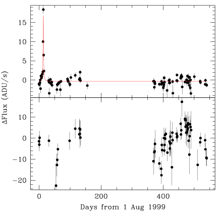
The POINT-AGAPE group uses the same data for their microlensing survey towards M31, although their pixel lensing technique is different (Paulin-Henriksson et al. Paulin03 (2003)). Based on the same two-year dataset, they find four high signal-to-noise microlensing events. Two of these events are also present in our sample, namely PA-99-N2, our event number 7, and PA-00-S4, our event number 11.

The fact that our sample of candidate microlensing events is much larger is caused by the severe selection criteria used by POINT-AGAPE, that limit the number of events found. For example, POINT-AGAPE demands FWHM timescales smaller than 25 days and much higher signal-to-noise than we. The following two events reported by the POINT-AGAPE team are not in our sample of candidate microlensing events.
$\bullet$ PA-99-N1
This event did not pass our filtering procedure because of too large variability in the i^′ baseline caused by a very closeby variable star. Our lightcurves of this event are shown in figure 5.
$\bullet$ PA-00-S3
Very close to the bulge of M31 the surface brightness becomes very high and our difference images become very noisy and of low quality. This event is located in a part of the field that is not used for the current analysis for this reason. In figure 1 the region that is not used in our analysis is indicated.

4 Discussion

Due to the nature of M31 microlensing, it is very difficult to determine the nature of the lensing object in individual microlensing events. In classical microlensing the mass of the lens, the relative motion of the lens with respect to the source and the distance to the lens are usually unknown and degenerate parameters. In difference-image lensing there is an additional unknown, namely the unlensed flux of the source. If a conclusion about the existence and/or nature of a MACHO population in the halo of M31 is to be drawn from a microlensing survey, statistical methods have to be used.

By modeling the population of stars that can be lensed and the population of objects that can act as lenses, predictions can be made about the rate of occurrence, the spatial distributions, and the timescales of microlensing events. All these data can be used to constrain the lens populations responsible for observed microlensing events (Baltz, Gyuk & Crotts Baltz03 (2003), hereafter BGC; Kerins et al. Kerins01 (2001)).

To compare our sample of candidate microlensing events with rate maps as published by BGC, the detection efficiencies and observing characteristics have to be carefully modeled, which will be done in a future paper. Instead of a full statistical analysis of the current sample, we restrict our discussion to a simple analysis of the spatial and timescale distributions of the candidate events to see if they are consistent with predictions for halo lensing and lensing by stars in M31.

4.1 Timescale distribution

Figure 6: For the 14 candidate microlensing events, the logarithms of the FWHM timescales are plotted against the local r^′ surface brightnesses. At high surface brightnesses the timescales tend to be shorter than in low surface brightness regions.

The timescale of a microlensing event depends on the relative velocities of the source and the lens and the size of the Einstein radius, which in turn depends on the mass of the lens and the geometry (eq. 3). In the case of M31 microlensing we can assume that $D_{OL}\leavevmode\nobreak\ =\leavevmode\nobreak\ D_{OS}$ and since the Einstein ring crossing time $t_{E}\leavevmode\nobreak\ =\leavevmode\nobreak\ 2R_{E}/v_{\perp}$ we get:

$$t_{E}\propto M_{L}^{1/2}D_{LS}^{1/2}v_{\perp}^{-1}$$ (1)

where $v_{perp}$ is the relative speed between lens and source projected on the sky. The $t_{FWHM}$ that we measure is related to $t_{E}$ according to equation 6.

For self-lensing, i.e. lensing by stars, this translates into a timescale distribution that varies spatially. In the bulge, velocities are relatively high and distances between lens and source relatively short (compared to lensing by halo objects), therefore event durations will be relatively short. In the disk, relative velocities are much slower and event durations longer than in the bulge. On top of that, the timescales are expected to rise when going to larger radii, since the random velocities of the stars in a galactic disk are proportional to the root of the surface density (Bottema Bottema93 (1993)). Roughly speaking we can say that average self-lensing timescales are inversely correlated with surface brightness; in higher surface brightness regions the timescales are expected to be shorter.

For halo lensing, relative velocities are higher than for disk-disk lensing, but because of the larger lens-source distance the event durations are still relatively long. Because the relative velocities and distances do not change much within the observed field, the timescale distribution of halo-lensing events should be spatially uniform. Plots of the expected timescale distributions for different lines of sight towards M31 are given by BGC for stellar self-lensing and halo lensing combined and reflect these trends.

In figure 6 we plot for our 14 microlensing candidates the logarithm of $t_{FWHM}$ versus the r^′ surface brightness at their locations. The candidate events close to the center of M31, in locations with surface brightness brighter than 19.5 $mag_{r\prime}\,arcsec^{-2}$, all have event durations in the order of a few days. Most of the candidates in the low surface brightness regions have significantly longer timescales. That this distribution is exactly what is expected for microlensing and the fact that the timescales are consistent with the timescales predicted by BGC are further indications that our sample of candidates consists of actual microlensing events.

4.2 Spatial distribution

Figure 7: Surface density map of long period variable stars in the surveyed area. Each chip was subdivided in 2x4 rectangles (300x324″), in which the number of variables with periods longer between 150 and 600 days was counted. Only stars with accurately determined periods were used and the edges of the chips were avoided to ensure only well sampled lightcurves were used, leaving 32,841 variables. The positions of the 14 microlensing candidates are indicated, as well as the major axis of M31.

The expected spatial distribution of stellar self-lensing events is strongly concentrated to the center because both the density of possible source stars and lenses is highest there. Furthermore, the spatial distribution is nearly symmetric from the far to the near side of the disk of M31 (BGC), so in the case of only self-lensing the number density of events should be the same at the same radius on both the far and near side. The stellar halo of M31 has not been taken into account by BGC, but is not expected to change the symmetry significantly, since, like the bulge, it acts both as a lens and as a source population. If the spheroid has the same M/L as the disk, for every event caused by a spheroid-lens and disk-source pair, there is a disk-lens and spheroid-source pair event, as is the case with disk-bulge and bulge-disk lensing (BGC). In case of heavy extinction in the disk, the spheriod could induce an asymmetry in the lensing rate.

Dark halo lensing on the other hand will induce an asymmetric microlensing distribution, because it only acts as a lens population. Due to the longer line-of-sight through the M31 halo towards the far side of the disk, the microlensing optical depth is much higher on the far side than on the near side. Therefore, an asymmetry in the density of microlensing events between the far and near side is a strong indication of a microlensing halo. Halo lensing is also more likely near the center because of the higher surface density of possible source stars, but drops off much more slowly, since the surface density of halo lenses should not drop off very quickly.

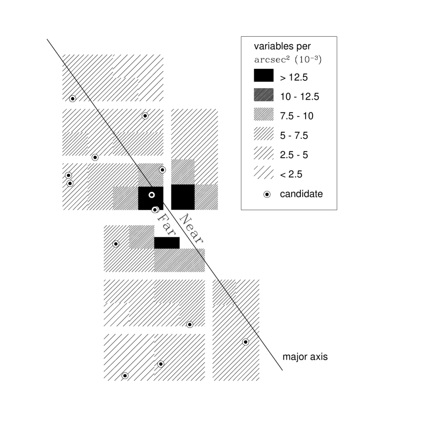
Without knowing the detection efficiency of microlensing events, the number of detected candidate events is hard to interpret quantitavely. Since the detection efficiency might vary with position, their spatial distribution is also hard to interpret. However, if we assume that the spatial distribution of variable stars is symmetric over M31, we can get an idea of the variation of the detection efficiency with position by looking at the spatial distribution of the detected variable stars. The variable stars that are most likely to be mistaken for microlensing are variables with periods longer than 150 days. In table 3 we present the detected numbers of variables with periods between 150 and 600 days, for 300x324^′′ subregions in our field of view. For each subregion the actual area, corrected for area lost due to bright stars and diffraction spikes, is also tabulated. In figure 7 we show the corresponding variable star density map, with the positions of the 14 candidate events plotted on top.

To select the long-period variables (LPVs) from the complete set of lightcurves, all lightcurves were checked for periodic behaviour using the Numerical Recipes (Press et al. numrec (1992)) algorithm based on the Lomb method (Lomb (1976)) for spectral analysis of unevenly sampled data. The lightcurves for which a periodicity between 150 and 600 days was found with very high significance were selected. In total 32,841 variables were selected, excluding the part of the south field close to the bulge and one other small part at the edge of the south field, where a very bright foreground star is located.

In the spatial distribution of the LPVs we see no surprises. The surface density of these objects is correlated with the surface brightness. Since we are interested in a possible asymmetry in the distribution of the candidate microlensing events, we compare the relative distributions of variables and events over the near and the far side of M31. We assume that the LPVs are a good tracer of the population of possible microlensing source stars and that the chances of detecting LPVs and microlensing events are the same. The detection efficiencies of both will depend on the surface brightness of the disk and be subject to extinction effects.

RA	DEC	LPV	Area	RA	DEC	LPV	Area
(J2000)	(J2000)	#	($\Box^{\prime}$)	(J2000)	(J2000)	#	($\Box^{\prime}$)
0:44:43.45	41:24:49.3	444	26.00	0:42:13.67	41:36:13.5	241	26.18
0:44:42.78	41:19:51.5	390	25.91	0:42:40.14	41:36:14.6	269	26.25
0:44:14.82	41:24:55.5	577	26.37	0:42:13.68	41:30:50.9	248	26.10
0:44:14.21	41:19:57.3	534	26.27	0:42:40.13	41:30:51.2	349	26.08
0:43:46.07	41:25:1.6	666	25.92	0:42:13.77	41:25:28.0	401	26.02
0:43:45.53	41:20:3.3	754	26.38	0:42:40.19	41:25:27.6	739	26.25
0:43:17.27	41:25:7.9	887	26.16	0:42:13.92	41:20:6.0	761	25.92
0:43:16.80	41:20:9.4	1340	26.36	0:42:40.32	41:20:5.0	1428	24.34
0:44:44.58	41:47:58.6	369	26.47	0:44:44.39	41:36:30.8	422	26.21
0:44:44.15	41:43:4.1	446	26.42	0:44:43.88	41:31:32.6	463	25.64
0:44:15.93	41:48:8.2	253	26.26	0:44:15.69	41:36:38.1	317	25.57
0:44:15.46	41:43:13.1	378	26.51	0:44:15.20	41:31:39.4	436	26.14
0:43:47.16	41:48:16.3	202	26.40	0:43:46.87	41:36:44.7	412	25.60
0:43:46.65	41:43:20.9	244	25.38	0:43:46.39	41:31:45.6	519	26.03
0:43:18.32	41:48:23.1	239	26.64	0:43:18.00	41:36:50.4	351	26.15
0:43:17.78	41:43:27.5	186	25.53	0:43:17.53	41:31:51.3	599	25.97
0:43:52.75	40:48:54.8	139	26.78	0:41:24.61	41:0:17.3	383	26.24
0:43:52.20	40:43:57.2	100	26.61	0:41:50.85	41:0:18.2	480	25.75
0:43:24.36	40:48:59.6	203	26.52	0:41:24.63	40:54:54.3	375	26.35
0:43:23.88	40:44:1.4	155	26.54	0:41:50.83	40:54:54.9	390	25.41
0:42:55.86	40:49:4.3	362	26.57	0:41:24.71	40:49:31.4	357	26.36
0:42:55.46	40:44:5.9	246	26.58	0:41:50.86	40:49:31.5	402	25.67
0:42:27.33	40:49:8.9	421	26.65	0:41:24.88	40:44:9.4	393	26.53
0:42:26.99	40:44:10.5	263	26.53	0:41:50.97	40:44:8.8	425	25.41
0:43:52.75	40:48:54.8	550	26.01	0:43:53.25	41:0:37.5	284	26.30
0:43:52.20	40:43:57.2	492	26.42	0:43:52.89	40:55:39.1	202	26.07
0:43:24.36	40:48:59.6	877	26.05	0:43:24.79	41:0:43.1	406	25.57
0:43:23.88	40:44:1.4	594	25.80	0:43:24.46	40:55:44.3	277	26.22
0:42:55.76	40:47:49.6	690	13.16	0:42:56.21	41:0:47.7	540	25.43
0:42:55.46	40:44:5.9	799	25.49	0:42:55.89	40:55:48.7	474	26.33
0:42:26.99	40:44:10.5	847	25.06	0:42:27.61	41:0:51.6	568	26.45
				0:42:27.29	40:55:52.4	564	25.73

Table 3: Number counts of detected long-period variable (LPV) stars. For each subregion, the coordinates of the center, the number of LPV’s and the area, corrected for area lost to bright stars and spikes, are given.

Figure 8: Upper panel: histogram of the surface densities of long-period variable stars (LPVs) in small 150x162^′′ regions on the far side of the M31 disk. The thin, black bars show in which LPV surface density bins the far side microlensing candidate events are located. Lower panel: histogram of the surface densities of LPVs in small 150x162^′′ regions on the near side. The thin, shaded bars show the numbers of candidate microlensing events predicted by scaling the numbers of far side events with the ratio of regions on the near and far side in each LPV density bin. In total 6 events are expected on the near side, but only 2 are detected, shown by the thin, black bars.

To investigate the different parts of the far and near side of the M31 disk that we sample, we divide each subregion in table 3 in 4 smaller 150x162^′′ pieces. In the upper panel of figure 8 we plot the distribution of the LPV surface densities of these small subregions. The smaller, black histogram shows the distribution of the far side candidate events over the LPV density bins. If the microlensing rates are intrinsically near/far side symmetric, as we assume the LPVs to be, the expected number of candidate events on the near side can be determined for each LPV density bin, by scaling the number of far side events. We can only do this for the low surface density bins, since the high surface density bins are not populated sufficiently. However, since close to the center of M31 the microlensing optical depth is dominated by stellar self-lensing they should not affect the symmetry of the spatial distribution. The lower panel of figure 8 shows the distribution of the subregions on the near side over the LPV density bins. The shaded histogram shows the distribution of the far side candidate events scaled to the near side LPV density distribution, and the black histogram the actual near side candidate events.

Whereas 6 near side candidate events are predicted from the distribution of the 9 far side events in areas with fewer than 10 LPVs per square arcsec, only 2 are detected. Thus, the distribution of candidate events seems to be more near/far asymmetric than the distribution of variable stars, which is an indication that it is a separate population of objects and not some kind of leakage from the population of LPVs. As argued before, the most likely explanation of such an asymmetry of microlensing events is dark halo lensing. The number of candidate events is still quite small, but the chance of finding a far:near split as strong as 9:2 is only 12%. It has been argued by Paulin-Henriksson et al. (Paulin02 (2002)) that candidate event 11 is possibly caused by a stellar lens in M32 and not by a lens in the halo. Doing the same calculation without candidate event 11, the chance of finding the 8:2 ratio is 16%.

5 Conclusions

In this paper we present the first 14 microlensing candidates from the MEGA survey and a preliminary discussion of their properties. Our photometry turns out to be sensitive to nearby variable sources in a way that causes us to miss out on events like PA-99-N1. It also leads to the necessity of a by-eye selection step in the filtering of the lightcurve database. Before the photometry is improved, enabling the filtering procedure to be automated and a detailed efficiency calculation to be done, we cannot draw firm conclusions based on the spatial distribution of our sample of candidate microlensing events. However, the spatial distribution of our candidate microlensing events is more near:far asymmetric, than would be expected from the spatial distribution of the detected long-period variable stars. Although the significance of this asymmetry is low, due to the small number of events and the lack of a detailed detection efficiency, the spatial distribution of the candidate microlensing events is suggestive of the presence of a microlensing halo.

Thus far we have only extracted candidate microlensing events from the 1999/00 and 2000/01 seasons. As a next step the remaining seasons will also be searched for microlensing events. Since we also observe with other telescopes than the INT, much more events will likely be detected when the data from the different telescopes are combined. Especially the sensitivity to short timescale events will benefit from merging the INT data with the data obtained with the telescopes of the MDM observatory, as they are supplementary in time coverage. Fainter events will also become easier to detect because the MDM data go deeper than the INT data, as do the data obtained with the KPNO 4m telescope.

Appendix A Microlensing event selection

A microlensing event caused by a single lens has a characteristic shape and a flat baseline. Such a standard microlensing lightcurve is called a Paczynski lightcurve (Paczynski Pacz86 (1986)) and is described by

$$F(t)\leavevmode\nobreak\ =\leavevmode\nobreak\ F_{0}\times A(t)\leavevmode\nobreak\ =\leavevmode\nobreak\ F_{0}\times\frac{u^{2}+2}{u\sqrt{u^{2}+4}}$$ (2)

where $F_{0}$ is the baseline, unlensed flux, $A(t)$ is the amplification, and $u$ is the projected distance between the lens and the source, in units of the Einstein radius. This Einstein radius depends on the geometry of the system and the mass of the lens and in the lens plane is given by:

$$R_{E}=\sqrt{\frac{4Gm}{c^{2}}\frac{D_{OL}D_{LS}}{D_{OS}}}$$ (3)

where $m$ is the lens mass and the Ds are the distances between observer, lens and source. Note that the amplification is always 1 or higher and independent of wavelength, meaning that microlensing is in principle achromatic and conserves the colour of the source. If the relative motion of lens and source is taken to be a uniform motion, then $u$ can also be written as:

$$u(t)=\sqrt{u_{min}^{2}+\left(\frac{t-t_{max}}{t_{E}}\right)^{2}}$$ (4)

where $u_{min}$ is the impact parameter, $t_{max}$ the time of maximum amplification and $t_{E}$ the Einstein time. This is defined as the time it would take the source to cross the Einstein radius. Since we are measuring only the flux difference of variable objects with respect to a template image, equation 2 transforms into:

$$\Delta F(t)\leavevmode\nobreak\ =\leavevmode\nobreak\ \Delta F_{bl}+F_{0}\times(A(t)-1)$$ (5)

where $\Delta F_{bl}$ is the baseline flux minus the flux on the reference image. As the crowding in M31 prevents the unlensed source flux from being measured, $\Delta F_{bl}$ is an unknown parameter that has to be fitted.

Furthermore, since the baseline flux is unknown and the microlensing event resolved only while magnified, it is very difficult to measure $t_{E}$ and $u_{min}$ (Gould Gould96 (1996); Baltz & Silk BaltzSilk00 (2000)), consequently these two parameters are highly degenerate, as shown in Figure 9. Instead, we fit the width of the peak at half of the maximum flux $t_{FWHM}$ (Gondolo Gondolo99 (1999)), which is related to $t_{E}$ by:

$$t_{FWHM}=t_{E}\cdot w(u_{min})$$ (6)

where $$w(u_{min})=2\sqrt{2f(f(u_{min}^{2}))-u_{min}^{2}}$$ (7)

with $$f(x)=\frac{x+2}{\sqrt{x(x+4)}}-1$$ (8)

We perform a four-parameter fit by letting $t_{FWHM}$ replace $t_{E}$ and $u_{min}$. To save computer time we assume a fixed value for $u_{min}$ and let $t_{E}$ float to fit for $t_{FWHM}$. Since there is some difference in the shape of the peak depending on $u_{min}$, we make fits for three values of $u_{min}$, namely 0.1, 0.3 and 1.0. These fits are sufficient for our selection procedure. Figure 9 shows that this range covers the range of possible shapes very well.

Figure 9: Differences in the Paczynski lightcurves for different values of the impact parameter $u_{min}$. The peak shape does not depend strongly on $u_{min}$, except from in the wings. In M31, where microlensing events are often only resolved while significantly magnified, the wings are usually not strongly constrained, meaning that it is difficult to measure $u_{min}$.

A.1 Selection of r^′ lightcurves

The selection of microlensing candidates was based on the goodness of fit of the standard Paczynski lightcurve fits to the 99/00 and 00/01 data. Based on the parameters of the best fits, the lightcurves are filtered in several steps, described below.
$\bullet$ Peak sampling
To be able to constrain event parameters it is important to sample the peak of the lightcurve well. We demand that at least the part of the peak where the flux is more than half of the peak flux lies completely within an observing season. For this the $t_{max}$ and $t_{FWHM}$ from the Paczynski fits are used. We also demand that there are at least 2 data points above 25% of the fitted peak flux. Furthermore, we calculate a ‘peak weight’ $P$ defined as the sum of all data points within the peak:

$$P\leavevmode\nobreak\ =\leavevmode\nobreak\ \sum_{i\in peak}\frac{\Delta F_{i}-\Delta F_{bl}}{\sigma_{i}}$$ (9)

where $\Delta F_{i}$ is the difference flux, $\sigma_{i}$ the error on the difference flux, and $\Delta F_{bl}$ is the difference flux of the baseline, as given by the Paczynski fit. All the points that are within 2 $t_{FWHM}$ of $t_{max}$ are considered to be in the peak and are used for this calculation. All points farther away from the center of the peak are considered to be part of the baseline. A minimum ‘peak weight’ $P$ of 25 is demanded.
$\bullet$ Peak significance
To exclude spurious detections, a minimum peak significance is demanded. The $\chi^{2}$ value of a flat line fit to the lightcurve is compared to the $\chi^{2}$ of the Paczynski fit. The difference between these two values has to be larger than 100 for selection.
$\bullet$ Peak width
Both a minimum and a maximum peak width are used. The minimum $t_{FWHM}$ of 1 day serves as an extra filter against spurious detections. Events with FWHM timescales longer than 150 days are also excluded, since with the current dataset the baseline is not well sampled. In practice, fits that give these very long timescales are usually caused by lightcurves that continue to rise at the end of an observing season.
$\bullet$ Baseline flatness
Microlensing events have flat baselines, contrary to periodic variables. The flatness of the baseline is checked by the goodness of fit of the Paczynski curve to the baseline, where the baseline is defined as that part of the lightcurve that is more than twice the $t_{FWHM}$ away from $t_{max}$. For this part of the lightcurve we use a cut of $\chi^{2}_{bl}/N<1.5$, where $N$ is the number of points in the baseline. The fits to the “empty” lightcurves that were used to assess the quality of the difference images showed that such a rather lenient cut is necessary, because our current photometry turns out to be quite sensitive to nearby variable objects which can cause some additional variability in some lightcurves.
$\bullet$ Goodness of fit
Finally, the shape of the peak must be consistent with microlensing, meaning that the Paczynski function must give a good fit. For the Monte Carlo simulations we find that a $\chi^{2}/N$ cut of 1.2 includes 90% of all events. However, secondary effects, like for example parallax effects, can influence the exact shape of the lightcurve. Also, the possibility of additional variability due to nearby variable objects must be taken into account. We use a rather lenient $\chi^{2}/N$ cut again, and since secondary effects will be stronger in high signal-to-noise events, this cut is also dependent on the ‘peak weight’ $P$ of the peak. The cut is described by $\chi^{2}_{pk}/N_{pk}<1.5+(\frac{P}{N_{pk}}-1)\times 0.1$, where $N_{pk}$ is the number of points in the peak, as defined above. Formally, a $\chi^{2}/N$ cut of 1.5 corresponds to a probability of 0.1% for the degrees-of-freedom in our fits, meaning that 99.9% of perfect microlensing lightcurves without any additional variability would pass this criterium.

Figure 10: Plot of the peak width and colour of the peaks that pass our r^′ filtering procedure. The different symbols refer to the $\chi^{2}/N$ value of the Paczynski fits to the i^′ lightcurves. Closed circles are $\chi^{2}/N<2$, open circles $2<\chi^{2}/N<3.5$, closed triangles $3.5<\chi^{2}/N<5$, and open triangles are $\chi^{2}/N>5$. The positions of the 14 candidate microlensing events are indicated with stars. Clearly visible is that the long period variable stars cluster around a $t_{FWHM}$ of 50 days and a i^′/r^′ flux of 4. For further filtering, the colour cut indicated by the dashed line was used. A $\chi^{2}/N$ of 2 was used as the base value of the $\chi^{2}/N$ cut applied to the Paczynski fits to the i^′ data. The remaining sample still contains lightcurves with variable baselines and events caused by bad pixels.

A.2 Colour information

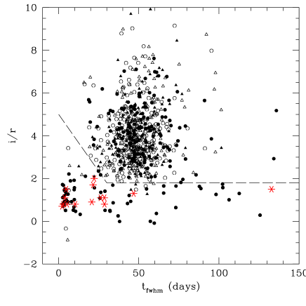
For several reasons the i^′ band data are important for the microlensing candidate selection. First, gravitational lensing is achromatic, so that the colour of the observed light in the difference images will not change during the microlensing event. Most periodic variable stars on the other hand, change colour during their pulsation cycles. Second, the long period variable stars like Mira’s that can otherwise easily be mistaken for microlensing events, are very cool and much brighter in i^′ than in r^′. Also the variability is much larger and therefore easier to see in i^′ than in r^′. Often, baselines that look flat in the r^′ data, clearly show variability in i^′. Third, most long period variables turn out to have similar colours, providing an easy way to filter them out of the lightcurve database.

Paczynski fits are done to the two-season i^′ lightcurves of the microlensing candidates selected from the r^′ data. The values for the wavelength-independent lightcurve parameters $t_{max}$, $t_{FWHM}$ and $u_{min}$ are taken from the fits to the r^′ data and used in the i^′ fits, since the r^′ data constrain these parameters better because of their superior quality. In the case of large colour changes during the event, these Paczynski fits to the i^′ lightcurves should be poor, indicative of a non-microlensing event.
$\bullet$ Colour cut
As mentioned before, long period variable stars have cool atmospheres and therefore are very red. In figure 10, the colours of the selected transients are shown as a function of the $t_{FWHM}$ of the Paczynski fits. The long period variable stars clearly stand out and cluster around a $t_{FWHM}$ of 50 and an i^′/r^′ flux ratio of 4. To remove the long period variables from the sample, a colour/$t_{fwhm}$ cut is used, indicated by the dashed line.
$\bullet$ Goodness of fit
In the i^′ data, the problems of crowding of the residuals in the difference images is worse than in the r^′ data, meaning that our photometry is influenced by nearby variables even more than in the r^′ data. Since the long period variables are very red, more are detected in the i^′ difference images and the residuals are much brighter. In figure 10 the transients are divided into four different bins depending on the $\chi^{2}/N$ value of the Paczynski fit to the i^′ data. A similar ‘peak weight’ dependent $\chi^{2}/N$ cut was applied to the i^′ lightcurves as to the peak of the r^′ lightcurve, but with a minimum $\chi^{2}/N$ of 2 in stead of 1.5: $\chi^{2}/N<2.0+(\frac{P}{N_{pk}}-1)\times 0.1$.

Appendix B Monte Carlo simulations

In order to develop and test the efficiencies of our lightcurve filtering procedures to select microlensing lightcurves from a large set of lightcurves, we performed Monte Carlo simulations of microlensing events. To be meaningful for comparison with the data, the simulated lightcurves should have the same time sampling and error distribution as the data. Furthermore, a broad range of time scales, times of maximum amplification, and peak brightnesses has to be sampled.

In total 170,000 lightcurves were simulated with random peak times, $t_{FWHM}$ of 1, 3, 6, 10, 30 or 60 days, seven different peak fluxes, and impact parameters of 0.1, 0.3, 1.0 or 10. With these four impact parameters most of all possible lightcurve shapes are sampled, as is illustrated in figure 9. For each simulated microlensing event, the time sampling and flux error bars were taken from a random real r^′ lightcurve, based on the 99/00 and 00/01 data. In this way, each simulated event has realistic characteristics, and the total sample of simulated events has the same observing charactistics as the total set of observed r^′ lightcurves. Standard Paczynski microlensing lightcurves were constructed, using the gaussian error bars taken from the real data lightcurve.

Figure 11: For all simulated microlensing lightcurves that pass our filtering procedure the fitted $t_{FWHM}$ and $t_{max}$ are plotted. From the clustering of the points it is clear that the fit program manages to recover the input widths of the simulations quite well. The gaps in the lightcurves show up as the events get shorter, while the period during which longer events can be detected is shorter than for the shorter events.

$t_{FWHM}$	Peak flux (ADU/s)
(days)	2	3.5	5	7	10	15	50
60	47	86	93	95	97	97	98
30	19	71	87	95	98	99	99
10	4	22	38	58	68	74	82
6	1	10	24	35	46	54	61
3	0	1	9	20	27	32	40
1	0	0	0	0	2	4	5

Table 4: The efficiencies of our r^′ lightcurve filtering procedure, in percent, for the simulated microlensing lightcurves.

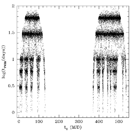
In table 4 the efficiencies of the selection of microlensing lightcurves are tabulated for all combinations of $t_{FWHM}$ and peak flux of the simulated events. For these detectability calculations simulated microlensing events were used for which the part of the peak higher than half of the peak flux lay completely within one observing season, which is one of our selecion criteria. It is clear that events with a peak flux lower than 3 ADU/s will hardly be selected. Also, events with a $t_{FWHM}$ lower than 10 days are relatively problematic. This large decrease in detectability for short timescale events is primarily caused by gaps in the time sampling of our lightcurves. This is shown in figure 11, where the fitted $t_{FWHM}$ and $t_{max}$ of the simulated microlensing lightcurves that pass the filtering procedure are plotted.

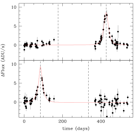
Since long period variable stars like Mira’s can mimic microlensing lightcurves, it is important to determine to what extent these lightcurves are selected by our microlensing selection procedures. Although Miras do not have a flat baseline on a logarithmic plot, on a linear flux scale the peaks are much sharper and the minima very near zero, thus they are typically below our noise level except for short periods around the peak. Mira variables have periods ranging from 130 to 500 days, with the most typical period being 270 days (Petit varstars (1987)). However, there are a number of Mira’s known with even longer periods (e.g. Jura et al. Jura93 (1993); Rosino et al. Rosino97 (1997)). Monte Carlo simulations of 120,000 Mira-type lightcurves were made with periods ranging from 150 to 550 days. The lightcurves were assumed to have a symmetric sawtooth shape in magnitude, with intrinsic variability amplitudes of 2, 4 or 6 magnitudes and 5 different flux variability amplitudes. Time sampling and flux errors were taken from real data lightcurves in the same way as for the microlensing simulations and starting phase of the variability was chosen randomly.

The filter efficiencies for the selection of simulated Mira lightcurves are tabulated in table 5. Variable stars with periods up to 200 days are not likely to be selected and confused for microlensing events, because at least two peaks will always be present in the lightcurve. Periods between 200 and 350 days are clearly a problem for our 2 year dataset. This is caused by the time coverage of our lightcurves, which for these periods often gives a peak in one of the observing seasons and a second peak just in between the seasons. This is why using the data from the third season is important; variables with these periods that show only one peak in a two season lightcurve will show a second peak in the third season. Two examples of simulated Mira lightcurves with periods of 250 days that mimic microlensing and pass our filters are shown in figure 12. Periodic variables with periods around 350 to 450 days are not selected because the fits are never very good and the baselines not flat. This is because a second peak will always have wings extending into one of the observing seasons. Longer period variables, however, can have only one peak in the lightcurve and a baseline that seems flat. Unfortunately, even with the third observing season data, these variables can still show one single peak and an otherwise flat baseline. Other characteristics, like colour and peak shape, have to be used to distinguish these variables from genuine microlensing events. For variable stars of all periods, the highest amplitude variables are least likely to be mistaken for microlensing events, because the difference in shape of the peak is detected better with higher amplitude.

The $t_{FWHM}$ values of the simulated Miras show that variables with longer periods have broader peaks, as can be expected. However, even the longest timescale simulated Miras show average $t_{FWHM}$ values between 30 and 40, while the real variables cluster around a $t_{FWHM}$ of 50 (Figure 10). Most detected real variables turn out to have more irregular peak shapes and lower peak heights than our simulated Miras, so that in reality long period variable stars are less likely to pass through our filtering procedure than table 5 suggests.

Period	Amplitude (ADU/s)
(days)	5	10	15	20	30
150	5	2	1	0	0
200	5	3	2	2	1
250	34	26	24	20	17
300	25	22	19	17	15
350	2	1	1	1	0
400	0	0	0	0	0
450	6	4	3	2	2
500	17	12	10	8	8
550	29	23	21	17	20

Table 5: The efficiencies of our r^′ lightcurve filtering procedure, in percent, for the simulated Mira lightcurves.

Figure 12: Two examples of simulated Mira lightcurves with periods of 250 days that pass our filters. The solid curves show the Paczynski fit to the lightcurves, and the dashed vertical lines indicate when the simulated Mira peaks. Both of the lightcurves have peaks in only one of the observing seasons, and therefore mimic microlensing quite well. A third observing season solves this problem for variables with periods around 250 to 300 days, but not very extremely long periods, i.e. longer than 500 days. Trends in the baseline like at the end of the first season in the upper lightcurve are often stronger in i^′ band than in r^′ band.

References

- (1) Alcock, C., Akerloff, C.W., Allsman, R.A. et al. 1993, Nature, 365, 621
- (2) Alcock, C., Allsman, R.A., Alves, D.R. et al. 2000, ApJ, 542, 281
- (3) Aubourg, E., Bareyre, P., Brehin, S. et al. 1993, Nature, 365, 623
- (4) Aurière, M., Baillon, P., Bouquet, A. et al. 2001, ApJ, 553, L137
- (5) Baillon, P., Bouquet, A., Giraud-Heraud, Y. & Kaplan, J. 1993, A&A, 277, 1
- (6) Baltz, E.A. & Silk, J. 2000, ApJ, 530, 578
- (7) Baltz, E.A., Gyuk, G. & Crotts, A.P.S. 2003, ApJ, 582, 30 (BGC)
- (8) Bertin, E. & Arnouts, S. 1996, A&AS, 117, 393
- (9) Bottema, R. 1993, A&A, 275, 16
- (10) Calchi Novati, S., Jetzer, Ph., Scarpetta, G. et al. 2003, A&A, 405, 851
- (11) Crotts, A.P.S. 1992, ApJ, 399, L43
- (12) Crotts, A.P.S. & Tomaney, A.B. 1996, ApJ, 473, L87
- (13) Crotts, A.P.S., Uglesich, R.R., Gyuk, G. & Tomaney, A.B. 2001, in ASP Conf. Ser. 237: Gravitational Lensing: Recent Progress and Future Go, eds. T.G. Brainerd & C.S. Kochanek, 243
- (14) Gondolo, P. 1999, ApJ, 510, L29
- (15) Gould, A. 1996, ApJ, 470, 201
- (16) Gyuk, G. & Crotts, A.P.S. 2000, ApJ, 535, 621
- (17) Jura, M., Yamamoto, A. & Kleinmann, S.G. 1993, ApJ. 413, 298
- (18) Kerins, E., Carr, B.J., Evans, N.W. et al. 2001, MNRAS, 323, 13
- (19) Lasserre, T., Afonso, C., Albert, J.N. et al. 2000, A&A, 355, L39
- (20) Lomb, N.R. 1976, Ap&SS, 39, 447
- (21) Milsztajn, A. 2002, Space Science Reviews, 100, 103
- (22) Paczynski, B. 1986, ApJ, 304, 1
- (23) Paulin-Henriksson, S., Baillon, P., Bouquet, A. et al. 2002, ApJ, 576, L121
- (24) Paulin-Henriksson, S., Baillon, P., Bouquet, A. et al. 2003, A&A, in press, astro-ph/0207025
- (25) Petit, M. 1987, Variable Stars, John Wiley & Sons
- (26) Press, W.H., Teukolsky, S.A., Vetterling, W.T. & Flannery, B.P. 1992, Numerical Recipes in C, Cambridge University Press
- (27) Riffeser, A., Fliri, J., Gössl, C.A. et al. 2001, A&A, 379, 362
- (28) Rosino, L., Ortolani, S., Barbuy, B. & Bica, E. 1997, MNRAS, 289, 745
- (29) Tomaney, A.B. & Crotts, A.P.S. 1996, AJ, 112, 2872