Oxygen Abundances in Metal-Poor Stars

Abstract

We present oxygen abundances derived from both the permitted and forbidden oxygen lines for 55 subgiants and giants with ${\rm[Fe/H]}$ values between $-2.7$ and solar with the goal of understanding the discrepancy in the derived abundances. A first attempt, using T_eff values from photometric calibrations and surface gravities from luminosities, obtained agreement between the indicators for turn-off stars, but the disagreement was large for evolved stars. We find that the difference in the oxygen abundances derived from the permitted and forbidden lines is most strongly affected by T_eff, and we derive a new T_eff scale based on forcing the two sets of lines to give the same oxygen abundances. These new parameters, however, do not agree with other observables, such as theoretical isochrones or Balmer-line profile based T_eff determinations. Our analysis finds that one-dimensional, LTE analyses (with published NLTE corrections for the permitted lines) cannot fully resolve the disagreement in the two indicators without adopting a temperature scale incompatible with other temperature indicators. We also find no evidence of circumstellar emission in the forbidden lines, removing such emission as a possible cause for the discrepancy.

1 Introduction

Oxygen is the third most common element in the Universe. It is copiously produced when massive stars explode as Type II supernova. This distinguishes it from Fe, which is also made in Type Ia SN, the accretion-induced explosions of white dwarfs. The [O/Fe] ratio therefore reflects the mix of stars that have contributed to the enrichment of a system. It has been used to diagnose the source of metals in X-ray gas in galaxies (Gibson et al., 1997; Xu et al., 2002) and in damped Ly$\alpha$ systems (Prochaska & Wolfe, 2002). Because Type II SN begin to explode more quickly than Type Ia SN after stars are formed, the O/Fe ratio after star formation begins is large at first, then declines as Fe, but little O, is contributed by the Type Ia SNe (Tinsley, 1979). This fact has been exploited to argue that Bulge formation lasted $<$ 1 Gyr (McWilliam & Rich, 1999) and star formation for dwarf galaxies happened in bursts (Gilmore & Wyse, 1991; Smecker-Hane & McWilliam, 2002). The fact that the oldest stars in our Galaxy have supersolar [O/Fe] ratios must be considered when measuring the ages of globular clusters (VandenBerg, 1985).

In particular, the [O/Fe] ratios in metal-poor stars in the Milky Way are important because they provide a look at the chemical evolution of the early Galaxy. We can use the O and Fe abundances to derive yields from Type II SNe, to adopt the correct isochrones for globular clusters, and to calculate the timescale for the formation of the halo. The [O/Fe] ratios in old Milky Way stars also provide a starting point for interpreting the abundances seen in high-redshift systems.

Unfortunately, the lines available in late-type stars are not ideal abundance indicators. The strength of the forbidden lines at 6300 Å and 6363 Å are gravity-dependent and are very weak in dwarfs and subgiants. The triplet of permitted lines at 7771-7774 Å have excitation potentials of 9.14 eV and therefore are weak in cool giants. For some evolutionary stages the permitted lines are also affected by NLTE effects (Kiselman, 1991; Gratton et al., 1999; Mishenina et al., 2000; Takeda et al., 2000). The OH lines in the ultraviolet and infrared regions of the spectrum are measurable in dwarfs and subgiants. However, OH is a trace species in these stars, and is particularly sensitive to inhomogeneities in temperature (Asplund & García Perez, 2001).

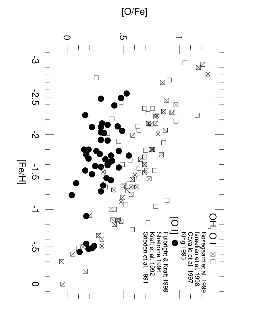
Figure 1: Sample oxygen abundances derived by previous studies to demostrate the systematic difference observed between the forbidden [O I] lines and the permitted O I and molecular OH lines.

Many studies using these abundance indicators show disagreement in the [O/Fe] vs. [Fe/H] relationship for stars with [Fe/H] $<-1.0$ (see Figure 1 for an incomplete, but demonstrative, summary). Because [O I] lines are stronger in giants and O I lines in dwarfs, studies using different indicators also use data from different types of stars. In general, the studies using permitted O I lines (Abia & Rebolo, 1989; Tomkin et al., 1992; Cavallo et al., 1997) and the UV OH lines (Israelian et al., 1998, 2001) in dwarfs and subgiants find a steep linear increase in [O/Fe] with decreasing [Fe/H]. Boesgaard et al. (1999) combined O I and UV OH measurements and found a slope of $-0.35$. In contrast, the [O I] lines in giants and subgiants give [O/Fe] values that plateau at $+0.35$ for [Fe/H]$<-1.7$ (Gratton & Ortolani, 1986; Barbuy, 1988). More recent analyses (King, 2000; Sneden & Primas, 2001) show instead a slight slope, but a difference of $\sim 0.5$ dex between the indicators at [Fe/H] $=-3.0$ remains. The O abundances measured from the infrared OH lines in dwarfs, subgiants, and giants produce similar values to the [O I] lines (Balachandran et al., 2001; Mishenina et al., 2000).

It is possible that the differences cited above are the result of intrinsic variations in the oxygen abundance between giants and dwarfs. However, studies of small samples of dwarfs with $-2.0<$[Fe/H] $<-0.5$ (Spite & Spite 1991, 7 stars; Spiesman & Wallerstein 1991, 2 stars) showed that the [O I] line in these stars gave an oxygen abundance 0.4-0.7 dex lower than that derived from the permitted lines in the same stellar spectra. Thus the discrepancy between forbidden and permitted lines cannot be ascribed alone to different intrinsic oxygen abundances in giants and dwarfs.

There have been many attempts to find another solution and to reconcile the results produced by the different sets of lines, either through finding the same slope and intercept in the [O/Fe] vs. [Fe/H] relation for different samples of stars or through finding the same O abundance using different lines in the same star. Oxygen abundances are sensitive to the adopted stellar parameters, so several studies have argued for improved methods for finding the parameters. King (1993) constructed new color-T_eff scales that produced effective temperatures that were 150–200 K hotter than those used by other investigators. These higher temperatures decreased the derived O abundance from the permitted lines so that they gave the same [O/Fe] ($\sim 0.5$ dex) at low metallicities seen in giants. Cavallo et al. (1997) also found that temperatures that were hotter by 150 K than their original temperature scale would erase the discrepancy in five turnoff dwarfs and subgiants with [Fe/H] $<-1.0$.

Recently, the gravities, rather than the temperatures, have come under scrutiny. King (2000) re-evaluated the [O/Fe] values for metal-poor dwarfs from Boesgaard et al. (1999) and Tomkin et al. (1992), in light of NLTE effects on Fe I (Thévenin & Idiart, 1999). King adopted gravities from Thévenin & Idiart (1999) and Axer et al. (1995) which were based on Fe I/Fe II ionization balance, but with NLTE corrections included for Fe I, and based the [Fe/H] scale on Fe II instead of Fe I. When this is done, the O I abundances show the same slight slope as the [O I] abundances, though they were still higher. For five unevolved stars with both [O I] and O I measurements, the O I-based abundances exceeded the [O I] by $+0.24\pm 0.05$ dex. Carretta et al. (2000) analyzed 40 stars (7 with [Fe/H] $<-1$) with measured O I and [O I] lines, ranging from dwarfs to giants. The O I abundances were corrected for NLTE effects using the results of Gratton et al. (1999), and they observed no difference between the two indicators on average, with the exception of the cool giants. The tendency of the permitted lines of giants to give higher abundances than the forbidden was attributed to deficiencies in the Kurucz (1992) models that were used in the analysis.

Nissen et al. (2002) obtained high-resolution, very high S/N ($>$ 400) data for 18 dwarfs and subgiants with $-2.7<$[Fe/H] $<-0.5$. Their equivalent width measurements have errors of $<0.3$ mÅ for the forbidden and $<1$ mÅ for the permitted lines. The quality of their data allowed the forbidden lines to be measured in higher-gravity metal-poor stars than before. When they used 1-D model atmospheres and NLTE corrections, the [O I], O I triplet and UV OH lines gave the same [O/Fe] vs. [Fe/H] relation. However, consideration of 3-D effects, in particular granulation, only reduced the oxygen abundance derived from the [O I] lines, and a disagreement remained at the level of 0.3 dex. Nissen et al. (2002) compared their [O/Fe] values in dwarfs with those in giants of the same metallicity. While the [O I] lines gave satisfactory agreement, the O I triplet lines in giants gave higher abundances than those seen in dwarfs and subgiants.

One metal-poor subgiant, BD +23 3130, has been subjected to intense scrutiny by several authors. Israelian et al. (1998) found [O/Fe] $=+1.17\pm 0.40$ for this star using the UV OH lines and O I triplet. Fulbright & Kraft (1999) argued that this was incompatible with the weakness of the [O I] line at 6300 Å, which yielded [O/Fe] $=+0.35\pm 0.20$. Cayrel et al. (2001) observed the 6300 Å line of this star at S/N $\sim$ 900 and measured an equivalent width of 1.5$\pm$0.5mÅ and found [O/Fe]$=0.71\pm 0.25$, halfway between the Israelian et al. (1998) and Fulbright & Kraft (1999) values. Israelian et al. (2001) revised the analysis using a log $g$ value 0.4 dex higher than their previous study. With this analysis, they found agreement among the UV lines, the [O I] line and the O I triplet. Nissen et al. (2002) used similar atmospheric parameters, but OSMARCS models also achieved agreement between the [O I] and UV OH lines with 1-D atmospheres, but not 3-D atmospheres. The studies of Nissen et al. (2002) and Israelian et al. (2001) suggest that a solution may be found in the application of correct stellar parameters and a consistent analysis of Fe and O using those parameters.

While using different indicators for different samples of stars increases the number of possible targets, especially at low metallicity, we will be looking instead at a sample that have both [O I] and O I lines. Using both sets of lines in the same star is important because star-to-star variations exist for oxygen and other element-to-iron ratios in metal-poor stars (Carney et al., 1997; King, 1997; Hanson et al., 1998; Fulbright, 2002). The most glaring example of this is the subgiant BD +80 245, whose permitted O I lines give a sub-solar [O/Fe] ratio at [Fe/H] $\approx-2.0$ (Carney et al., 1997). Also, such a tactic avoids the question of whether oxygen has been depleted by internal mixing in giants, which means that they can be included in the sample. Therefore, a more rigorous way to insure both the permitted and forbidden oxygen lines truly give the same results is to use both lines in the same stars.

The recent studies of Israelian et al. (2001) and Nissen et al. (2002) showed that agreement between the oxygen abundance given by O I and [O I] could be reached, at least for turnoff dwarfs and subgiants, for their particular choices of 1-D atmospheres. However, because of the weakness of the [O I] line in dwarfs and subgiants, there are only six stars in these two papers that have both [O I] and O I measurements. We chose to focus on subgiants and giants to obtain a large, homogeneous sample of stars with both sets of lines measured, including a number with [Fe/H] $<-1.5$. This will also test whether the successes with the dwarfs and subgiants can be replicated, or whether, like Carretta et al. (2000), the analysis of cool giants will produce different oxygen abundances. We have taken advantage of the very high resolution (R $\sim 130000$) Gecko spectrograph on CFHT to obtain equivalent widths for the [O I] lines for a sample of 55 stars, mostly subgiants and giants, with [Fe/H] between $-$2.7 and solar. Additional spectra and literature sources have been included so that all 55 stars have measurements of both the permitted and forbidden oxygen lines.

The data set presented here provides a strong test of any attempts to reconcile the indicators. We will begin our analysis by measuring the magnitude of the difference in these two oxygen abundance indicators when we adopt atmosphere parameters with T_eff from colors and log $g$ from isochrones. We find that the familiar pattern of O I lines giving higher O abundances than the [O I] lines reasserts itself. Next, we examine whether changing the assumptions of the analysis, in particular the temperature scale, eliminates the measured difference. We then use the knowledge of the behavior of the lines to create an ad hoc parameter set that, within the assumptions of the analysis, results in agreement between the indicators. Finally, we discuss whether this ad hoc parameter scale is realistic when compared to other observables for the target stars.

2 Methodology

An exhaustive study of all the possible solutions to the oxygen abundance problem is beyond the scope of a single paper. We therefore concentrate on following up the apparent successes of parameter-based solutions in the recent works mentioned in the Introduction.

Our analysis follows the following assumptions:

1) The atmospheres of stars can be described by one-dimensional, plane-parallel models in LTE. For most of this work, we will use Kurucz (1995) models. We use the MOOG stellar abundance package (Sneden, 1973) for the analysis. We adopt $\log{\rm n(Fe)_{\odot}}=7.52$ and $\log{\rm n(O)_{\odot}}=8.69$. The later value is based on the reanalysis of the solar [O I] by Allende Prieto et al. (2001), which takes in account the contamination of the 6300 Å [O I] line by a Ni I weak line.

2) Non-LTE effects limit the usefulness of Fe I lines (Thévenin & Idiart, 1999) in metal-poor stars. Non-LTE conditions also affect the permitted O I lines, but for the purposes of this experiment we will assume the abundance corrections of Takeda et al. (2000) adequately compensate for the departures from LTE. We also assume the lines of Fe II are free of non-LTE effects and will be used as the primary Fe abundance indicator.

3) Within the assumptions above, we will assume the solution to the problem can be found by the application of the correct atmospheric parameters for the stars. This assumption is similar to the solution put forth by King (2000).

The methods employed here are similar to those taken by Nissen et al. (2002) and King (2000), but their samples contain only warm (T_eff$>5600$ K) turn-off and subgiant stars, and only have 11 stars between them with both forbidden and permitted lines.

3 Target Star Selection and Observations

The Gecko echelle spectrograph on the Canada-France-Hawaii Telescope (CFHT) delivers spectra with resolution of $\sim 130000$, with a dispersion of $0.018$ Å per 13.5 $\mu$m pixel. Only one spectral order is observable at a time (selected by a narrow-band filter), meaning only a $\sim 75$ Å region is observed per exposure with the thinned 2048x4096 pixel detector. The Gecko data were obtained over 6 nights in April and September 2001. In both runs, the spectra covered the wavelength range from 6290–6370 Å, covering both the 6300 Å and 6363 Å lines.

The primary candidate list was created in a similar manner as the target list of Fulbright (2000), using literature lists of known metal-poor stars, such as Bond (1980), Carney et al. (1994), etc. The list was then culled of stars where we estimated that one of the two sets of lines would be undetectable.

The spectra were reduced using normal IRAF routines. Although previous work has shown that the scattered light effect in Gecko is less than 1%, special care was taken in its removal. A wavelength solution was applied using ThAr lamps taken at the beginning and end of the night. The variation in the wavelength of the telluric O₂ features between spectra is less than 100 m s^-1. Details of the individual observations are given in Table 1.

Because the 6300 Å feature lies within a band of telluric O₂ lines, it was sometimes necessary to remove these telluric lines from the spectrum. During the observation runs, spectra of bright, rapidly-rotating (vsini $>250$ km s^-1), spectral type B or A stars were observed. These spectra were used to divide out the telluric O₂ features (some sample spectra are shown in the Appendix). For most stars the division was cosmetic, because the [O I] line was not contaminated and the very high resolution and dispersion of the Gecko spectrograph lessens the probability of contamination.

Langer (1991) suggested circumstellar [O I] emission may play a role in the discrepancy. We did not observe any sign of stellar [O I] emission in our spectra, a point which we examine this point further in the Appendix.

Additional data to measure the Fe and O I lines were obtained with the Lick 3-m and KPNO 4-m with their respective echelle spectrographs. The new data taken with the Hamilton spectrograph at Lick were obtained in the same way as the previous data (see Fulbright 2000 and Johnson 2002 for more details). The echelle data from KPNO were obtained in January 2002 with a resolution of $\sim 40000$ and covers the wavelength range from 4480 to 7850 Å. Included in the KPNO data is a spectrum of the asteroid Vesta, which provides a solar spectrum taken as if the Sun was a point source.

4 Line Measurement

The equivalent widths (EW) values of the 6300 and 6363 Å [O I] lines were measured using both Gaussian fits and integrations. The EW of the 6300 Å line for BD +23 3130 was adopted from Cayrel et al. (2001). The EW values for the permitted O I lines were measured in the non-Gecko data or taken from literature sources or a combination of both. Table 2 gives the oxygen EW values for the stars analyzed in this paper. The EW of the 6300 Å [O I] line has been corrected for contamination by the 6300.34 Å Ni I line (see Section 6.1).

We adopt the Lambert (1978) $gf$-values for the 6300 and 6363 Å forbidden lines ($\log{gf}=-9.75$ and $-10.25$, respectively), and the Bell & Hibbert (1990) $gf$-values for the 7772, 7774, and 7775 Å permitted lines ($\log{gf}=+0.36$, $+0.21$, and $-0.01$, respectively). The Fe line list of Fulbright (2000) is used here. The atomic data for the Fe I lines are from O’Brian et al. (1991) and the Oxford group (Blackwell et al., 1982, and references therein), while the Fe II lines have data from Blackwell et al. (1980) and Moity (1983). Slight modifications have been made to the $gf$-values to improve consistency between sources, as described in detail by Fulbright (2000). Many of the target stars have been analyzed by the authors before (Fulbright, 2000; Johnson, 2002). We adopt the Fe EW values from those papers. The Fe EW values for the previously-unpublished stars are given in Table 3a and 3b (available in the electronic version only).

The oxygen abundances found for the solar analysis are larger than the adopted solar oxygen abundance of Allende Prieto et al. (2001) by 0.14 (forbidden) and 0.10 (permitted) dex. We could change the $gf$-values of the lines to reflect these differences, but the value of 8.69 comes from a 3-D analysis, which we do not do here. Allende Prieto et al. report that using a one-dimensional model would increase the resulting solar oxygen abundance by 0.08 dex, in reasonable agreement with the solar abundance derived by the 1-D analysis conducted here. Therefore, we choose not to do a differential abundance analysis.

For this paper, the ratio of the abundances given by the two oxygen indicators is more important than the absolute abundance. Using the present $gf$-values, the solar analysis yields a forbidden line oxygen abundance 0.04 dex larger than that obtained permitted lines. However, if we assume that all of the uncertainty is from line measurements error, we get an uncertainty for the ratio of 0.06 dex (dominated by the uncertainty in the EW of the 6300 Å line). Therefore, we believe that a change in the $gf$-values is not warranted by the analysis. If the $gf$-values were changed to force agreement, the needed $\Delta$T_eff vaules in Section 7 would be increased by about 35 K.

5 Stellar Parameters

5.1 Effective Temperatures

Initially, we will analyze the oxygen and iron abundances using stellar parameters derived from two photometric temperature scales: Alonso et al. scale (1996 for dwarfs and 1999 for giants) and Houdashelt et al. (2000). The Alonso scales are based on the Infrared Flux Method (IRFM) of Blackwell et al. (1979), while the Houdashelt scale is based on synthetic spectra with zero points based on observations.

The input photometry for these relationships came from a variety of literature sources. The B$-$V and V$-$I data are from the Hipparcos/Tycho catalog, and the ubyv$\beta$ photometry is from Hauck & Mermilliod (1998). K colors were taken from the papers of Alonso et al. (1994 and 1999), Carney et al. (1983), Laird et al. (1988), and the 2MASS Point Source Catalog. Many V-R colors were taken from Stone (1983), while others come from Laird et al. (1988) and Carney et al. (1983).

Measurements of the reddening were taken from literature sources such as Anthony-Twarog & Twarog (1994) and Carney et al. (1994). Other reddenings were derived using ubvy$\beta$ photometry and the calibration of Schuster & Nissen (1989), although the limits of that calibration exclude many evolved stars. We adopt E(B$-$V) $=1.37$ E(b$-$y) and the transformations of Reike & Lebofsky (1985). For the 8 stars for which we could not find or derive reddening estimates, we assume zero reddening.

The final dereddened colors are given in Table 4, while the calculated and adopted T_eff values are given in Tables 5 and 6. In all cases the T_eff values were only accepted if the star’s parameters were within the limits of a given color’s calibration. Because both Alonso and Houdashelt give different calibrations for giants and dwarfs, stars with derived log $g$ $>3.5$ were considered dwarfs while the remaining stars were considered giants. While we initially intended to adopt the mean T_eff value for the analysis, the T_eff values derived from the (V$-$I) colors were consistently higher. Additionally, the spread between the results for the different T_eff$-$color relations for individual stars was sometimes very large, most likely due to problems with the photometric data. Therefore we ignored most of the results from the (V$-$I) T_eff$-$color relation and other discrepant points when deciding which T_eff value to adopt for each star. The final values have been rounded to the nearest 25 K increment. For convenience, we list the final log $g$, [m/H], and $v_{t}$ values for each star in Tables 5 and 6.

We have assigned a measure of the uncertainty in T_eff to each star. In most cases, the value is the standard deviation of the T_eff values used in the final calculation of the adopted value. While the agreement between the individual T_eff$-$color relationships for some stars is quite good, we believe that the uncertainty in the photometric data and the calibrations of the T_eff$-$color relationships place a lower limit of 75 K on the T_eff uncertainty.

5.2 Surface Gravities

Many traditional abundance analyses derive surface gravities from forcing agreement in the abundances derived from the Fe I and Fe II. Thévenin & Idiart (1999, hereafter TI99) and Allende Prieto et al. (1999) both present evidence that the Fe I lines in very metal-poor stars suffer from non-LTE effects. Therefore LTE analyses of these lines do not give reliable abundances. We will derive surface gravities for our stars from the mass ($M$), absolute V magnitude (M_V), a bolometric correction ($BC$), and effective temperature (T_eff):

$$\log{g}=\log{\frac{M}{M_{\odot}}}-0.4(M^{\odot}_{\rm bol}-M_{\rm V}-BC)+$$

$$4\log{\frac{\rm T_{eff}}{\rm T_{eff}^{\odot}}}+\log{g_{\odot}}.$$ (1)

We adopt ${\rm T_{eff}^{\odot}}=5770$ K, $\log{g_{\odot}}=4.44$ and $M^{\odot}_{\rm bol}=4.72$. The adopted stellar masses were based mostly on the star’s assumed position on the appropriate-metallicity 12 Gyr VandenBerg (2000) isochrones (adopting a 10 or 14 Gyr isochrone results in negligible differences). However, several stars are likely to have evolved beyond the first-ascent giant branch and probably have undergone some form of mass loss. For these stars we adopt $M=0.6$ M_⊙ (see below). Bolometric corrections were calculated from Alonso et al. (Alonso et al. 1995 for dwarfs and Alonso et al. 1999 for giants).

The adopted M_V magnitude, especially for giants, can be fairly uncertain. For stars for whose Hipparcos parallax value has $\sigma_{\pi}/\pi<0.25$, we adopt the Hipparcos M_V value. Many of the remaining stars, especially the giants, have poor Hipparcos parallax determinations. However, Hanson et al. (1998) and Anthony-Twarog & Twarog (1994) derive M_V values for many giants and subgiants. Hanson et al. (1998) used Hipparcos parallax data to improve the M_V values derived by Bond (1980), which themselves were based on fits to globular cluster color-magnitude diagrams. Anthony-Twarog & Twarog (1994) derived distances using Strömgren photometry and Norris et al. (1985) relationships between M_V, [Fe/H] and color.

For all the non-horizontal branch (HB) stars, we also derived estimates for the M_V value by using their dereddened colors to place them on the 12-Gyr VandenBerg (2000) isochrone appropriate for their estimated [Fe/H] value. For stars with estimated [Fe/H] values lower than the $-2.31$ limit of the isochrone grid, the [Fe/H] $=-2.31$ isochrone was used.

A number of the target stars are HB or asymptotic giant branch (AGB) stars, which affects their adopted M_V and mass values. Following Eggen (1997), we identify potential post-RGB candidates in the distance-independent $c_{0}$ vs. $(b-y)_{0}$ plane (see Figure 2). The locus of subgiant and first-ascent giants is traced by ubyv isochrones kindly provided by Clem & Vandenberg (private communication).

For the stars that fell into the HB or AGB regions of the diagram, we adopt a mass of 0.6 M_⊙ following Gratton (1998). The adopted M_V value for the assumed HB stars near the ZAHB locus follows M${}_{\rm V}^{\rm HB}=0.19($[Fe/H]$+1.5)+0.61$ (Gratton, 1998). For the evolved HB and AGB stars, the method of determining the M_V value was no different than other stars, although a lower limit to the M_V value was placed by the appropiate M${}_{\rm V}^{\rm HB}$ value.

The M_V value for stars without high quality Hipparcos parallaxes or stars not on the HB was based on a combination of the Hanson et al. (1998), Anthony-Twarog & Twarog (1994) and isochrone-derived values. Table 7 lists the M_V values from the various sources, as well as the final adopted M_V and stellar mass values. The errors in M_V were calculated from the Hipparcos parallax or estimated from the source papers. For the HB stars, an error of 0.2 mag was adopted to account for uncertainties in the M_V$-$[Fe/H] calibration and any evolution above the horizontal branch. A color–absolute magnitude diagram for the final adopted values is shown in Figure 3. For reference, a 0.5 mag error in M_V contributes a 0.2 dex uncertainty in log $g$.

5.3 Atmospheric [m/H] and $v_{t}$ Values

An estimate of the [Fe/H] value for each star was taken from the literature source of the star. The adopted atmospheric [m/H] value was $\sim 0.1$–$0.2$ dex higher because most metal-poor stars have enhancements in the so-called $\alpha$-elements (O, Mg, Si, Ca, etc.), which provide more free electrons than are accounted for in the solar ratio models. After the first abundance analysis iteration of Fe lines, the [m/H] value was based on the [Fe/H] value derived from the Fe II lines.

We use the $v_{t}$ value that gave a flat distribution of derived Fe I abundances as a function of line strength. Errors in the adopted $v_{t}$ value have negligible effect on the derived oxygen abundances because most of the oxygen lines are weak.

6 Abundance Analysis

6.1 NLTE and Ni corrections

We use the NLTE corrections of Takeda et al. (2000). The grid of corrections only includes stars warmer than 4500 K, but our sample includes stars several hundred degrees cooler than that limit. For stars outside the Takeda et al. grid, we have calculated corrections using an extrapolation from the nearest grid points.

Gratton et al. (2000) and Mishenina et al. (2000) also derived NLTE corrections for oxygen lines. A comparison of the Gratton et al. and Takeda et al. corrections for the 7772 Å O I line is shown in Figure 4. We calculated the comparisions by assuming the same O I line strength using the listed [O/Fe]_LTE value for each metallicity. The only large difference between the two calculations is for the hot, low-surface gravity stars. Adopting the Gratton et al. correction for the HB stars in our sample would result in a reduction of the NLTE correction by less than 0.15 dex.

The 6300.31 Å [O I] line is blended with a Ni I line at 6300.34 Å. While the Ni line is fairly weak, it does affect the derived oxygen abundance in the Sun (Allende Prieto et al., 2001). As a correction, we have subtracted the estimated strength of the Ni I line (calculated using the adopted Alonso T_eff scale models and assuming [Ni/Fe] = 0) from the measured 6300 Å EW. In general the correction was only a small fraction ($<10\%$) of the adopted EW value, only being significant in metal-rich stars like the Sun. The EW values for the 6300 Å line given in Table 2 reflect the corrected values.

6.2 Error Analysis

6.2.1 Equivalent Width Errors

The weakness of [O I] and O I lines in metal-poor stars means that EW errors can dominate the error budget and need to be considered carefully. Cayrel (1988) gives a useful derivation of the error in EW. We write the EW as

$$EW=\delta x\Sigma{}(C_{i}-r_{i}),$$ (2)

where $\delta x$ is the dispersion in Å/pix, $C_{i}$ is the value of the continuum, and $r_{i}$ is the intensity at pixel $i$. This is summed over the $n$ pixels which contain absorption in the line. In practice, we summed over 15 pixels in the Gecko case and 7 or 8 pixels for the KPNO or Lick data, respectively. The error in the EW, taking into account that the errors in $C_{i}$ are completely correlated is

$$\delta EW^{2}=\delta x^{2}\left(\Sigma\delta r_{i}^{2}+n^{2}\Sigma\delta C_{i}^{2}\right).$$ (3)

We used the S/N of the 6300 Å region as the measure of $\delta r_{i}$. $\delta C_{i}$ is also based on the S/N, but because we averaged $\sim$ 50 pixels around the oxygen lines to locate the continuum, the error in continuum is $\delta r_{i}/\sqrt{50}$. We determined the S/N by actually measuring the s.d. in the spectra, rather than relying on the photon statistics, though in practice they were the same. Using the S/N ignores other sources of error, in particular scattered light, but as discussed in §3, the Gecko spectrograph set up minimizes the impact of scattered light.

We can check our calculations of the EW error in two ways. First, for 38 stars, we measured all three O I permitted lines and then determined the expected error in the average abundance both by using the errors derived from Equation 3 and by calculating the standard deviation in the mean for those three lines. There was encouraging agreement, usually to within 0.02 to 0.03 dex. Second, we compared our EWs to previous published measurements (Figure 5). For the 6300 Å line, we find an average offset of $-2.4$ mÅ with a rms scatter of 3.9 mÅ. The average offset for the 6363 Å is 0.0 mÅ with an rms scatter of 2.2 mÅ. A number of Gratton et al. (2000) EW values are higher than the Gecko observations, while the one discordant 6363 Å value, from BD +30 2611 (=HIP 73960), has a 6300 Å EW that agrees with the Kraft et al. (1992) value. The ratio between our EW values for the 6300 and 6363 Å lines in this star do not follow the expected 3-to-1 ratio (37.7 mÅ vs. 17.6 mÅ), but the Gecko spectrum does not show any indication of the source of the error. The lines joining the EW values derived for the same star indicate many cases of large scatter (up to 50%) among studies even when our data are not considered.

The uncertainty in our EW values from our statistical calculation (generally on the order of 1 mÅ or less) cannot explain the rms deviations seen in Figure 5. The most likely cause for much of the scatter seen is the lower quality of the previous data. The Gecko data presented here are at higher resolution and dispersion than the previous data, have negligible scattered light, and have minimal O₂ contamination problems.

6.2.2 Stellar Parameter-Based Errors

To measure the effects of systematic parameter errors on the oxygen and iron abundances, we ran a series of models for each star: one with the T_eff value raised by 200 K, one with the log $g$ value raised by 0.3 dex, one with the [m/H] value raised by 0.3 dex, and one with the $v_{t}$ value raised by 0.3 km s^-1. The abundances from each of these individual runs were compared against the results of the original run.

The overall effect of the parameter changes on the whole sample of stars is given in Table 8. Both the permitted and forbidden lines are affected by the T_eff and log $g$ values. The choice of T_eff is the most important parameter affecting the [O/Fe] ratios and the difference between the two oxygen indicators. The [m/H] value is slightly significant, but it is unlikely that a 0.3 dex systematic error in the [m/H] value would occur in practice.

The effects of various parameter changes on the forbidden and permitted oxygen and Fe II abundances as a function of T_eff, log $g$, and [Fe/H] are given in Plots 6–8 for each star in the sample.

The most important feature in the plots is that a T_eff change has opposite effects on the permitted and forbidden line abundances, while the other parameter changes affect the two indicators in similar ways. The figures also show that a systematic error in the surface gravity affects the abundance indicators by the same amount, but a systematic T_eff error affects giants more than dwarfs, and metal-poor stars more than metal-rich stars. An error in [m/H] affects metal-rich stars more than metal-poor ones. Fe II mostly behaves like [O I] when [m/H] is changes, but more like O I when T_eff is altered. These results indicate that great care must be taken when comparing the results from different evolutionary status. Systematic parameter problems affect some stars, such as metal-poor giants, more than others.

6.2.3 Random Errors in [O/H] and [O/Fe]

While systematic effects may be the most important factors in resolving the the disagreement between the forbidden and permitted lines, it is important to know the random errors associated with the O abundances to determine the significance of discrepancies. We consider random errors in EWs, T_eff, log $g$, and [m/H] of the model. The abundance error due to $v_{t}$ is less than 0.03 dex and will be not considered in our analysis. We modify the formula from McWilliam et al. (1995):

$$\sigma^{2}_{log\epsilon}=\sigma^{2}_{EW}+\left({\partial log\epsilon\over\partial T}\right)^{2}\sigma^{2}_{T}+\left({\partial log\epsilon\over\partial\rm{log}g}\right)^{2}\sigma^{2}_{\rm{log}g}+$$

$$\left({\partial log\epsilon\over\partial\rm{[m/H]}}\right)^{2}\sigma^{2}_{\rm{[m/H]}}+{}{}2\biggl{[}\left({\partial log\epsilon\over\partial T}\right)\left({\partial log\epsilon\over\partial\rm{log}g}\right)\sigma_{T\rm{log}g}+$$

$$\left({\partial log\epsilon\over\partial\rm{[m/H]}}\right)\left({\partial log\epsilon\over\partial\rm{log}g}\right)\sigma_{\rm{log}g\rm{[m/H]}}+{}$$

$${}\left({\partial log\epsilon\over\partial\rm{[m/H]}}\right)\left({\partial log\epsilon\over T}\right)\sigma_{T\rm{[m/H]}}\biggr{]},$$ (4)

where $\sigma_{T\rm{log}g}$, for example, is defined as

$$\sigma_{T\rm{log}g}=\frac{1}{N}\sum_{i=1}^{N}\left(T_{i}-\overline{T}\right)\left(\rm{log}g_{\it i}-\overline{\rm{log}g}\right).$$ (5)

The partial derivatives were calculated in Section 6.2.2. Equation 1 shows that log $g$ is dependent on T_eff. The extent to which our uncertainties in T_eff and log $g$ are correlated depends on the magnitude of the error in M_V. Therefore, for each star in our sample, we did a Monte Carlo experiment where we allowed T_eff and M_V to vary based on their errors, then calculated log $g$ using Equation 1, then placed into Equation 5 to calculate $\sigma_{\rm T\rm{log}g}$. Other $\sigma$ values were determined in the same manner.

The errors in ratios such as [[O I]/Fe] can be appreciably smaller than the addition in quadrature of [O I] error and Fe II error, because they have similar sensitivities to changes in atmospheric parameters. We used Equation A20 from McWilliam et al. (1995), modified to include [m/H] errors, to calculate abundance ratio errors. The error bars in Figure 10 are calculated using this formula. No errors were calculated for the Sun.

6.3 Results for Alonso and Houdashelt Scales

The abundance results from the Alonso and Houdashelt parameter scales are shown in Figures 9 and 10. In Figure 9, neither scale results in both sets of oxygen lines giving the same abundance for all stars, although the warmer Houdashelt scale does a better job. The unweighted mean value of [O_p/O_f] ($\equiv\log{\rm n(O_{p})}-\log{\rm n(O_{f})}$) for the Alonso scale is $+0.35\pm 0.03$ (sdom), and $+0.09\pm 0.04$ (sdom) for the Houdashelt scale. In Figure 10, [O_p/O_f] is shown as a function of the stellar parameters.

The ratio [O_p/O_f] is larger for the cooler, lower surface gravity giants than for the warmer, higher gravity subgiants and dwarfs. Both least-squares and Spearman rank-order tests confirm that there are highly significant anti-correlations between [O_p/O_f] and these two parameters. These same tests do not support a correlation between [O_p/O_f] and [Fe/H]. This is in contrast to previous studies (see Figure 1) in which the value of [O_p/O_f] increases with decreasing [Fe/H]. In these earlier studies, the forbidden oxygen abundances came from giants and the permitted abundances came from dwarfs. Our result suggests that the growth of [O_p/O_f] with decreasing [Fe/H] is at least partially due to comparing stars of different evolutionary status.

In Figure 10, it appears that the [O_p/O_f] distribution for the Houdashelt scale is bimodal, with some stars clustered at [O_p/O_f] $=+0.5$ and the majority around [O_p/O_f] $=0.0$. Indeed, a KMM test (Ashman et al., 1994) finds that there is a 96% probability that two Gaussians fit the distribution better than a single Gaussian. The best fit model would place 12 stars in a group with a mean of $+0.51\pm 0.12$, and the remaining 43 in a group with a mean of $-0.02\pm 0.17$. While this is only a two-sigma result, understanding why the 12 stars (all with [O_p/O_f] $>+0.3$) are outliers may yield clues to the origin of the overall problem.

Unfortunately, a detailed investigation into the properties these 12 stars found nothing striking about these stars except that they all have log $g$ $<3$ and [Fe/H] $<-1$. These 12 stars are also among the stars with the highest [O_p/O_f] values when the Alonso T_eff scale is applied, so the origin of the high [O_p/O_f] value may be unrelated to the Houdashelt scale. Checks for binarity, evolutionary status, systematic errors with the photometry, EW measurements, M_V and reddening determinations, etc. did not yield any noticeable pattern for the 12 stars, especially one that would lead to such a tight clustering of outliers.

It can be concluded here that both the Alonso and Houdashelt scales fail to totally resolve the discrepancy. While the warmer Houdashelt scale comes closer than the Alonso scale, there are still several giant stars that have large [O_p/O_f] values. Two possible reasons for the failure are: First, there is missing input physics in the analysis and an additional correction to the abundance results is necessary, or, second, the physics of the analysis is adequate, but the input parameters for the models are incorrect.

Full exploration of the first option is beyond the scope of this paper, but one simple explanation is that the NLTE corrections adopted here are simply wrong. To correct the differences seen in Figure 10, NLTE corrections would have to be much larger for low-gravity stars. The corrections of Gratton et al. (2000) are nearly identical to those of Takeda et al. (2000) (see Figure 4) for this type of star, so the choice of NLTE correction does not to affect the results. In section 6.4, we will look at the effect of changing our choice of stellar atmospheres. In Section 7, we will assume the second option is correct and calculate stellar parameters that reconcile the indicators.

6.4 MARCS vs. Kurucz Atmospheres

As mentioned above, the analyses to this point have been done using Kurucz atmospheres. The MARCS grid of stellar atmospheres (Bell et al., 1976) are an independent calculation of one-dimensional, plane-parallel atmospheres. To test whether the adopted atmosphere grid makes a significant difference, we re-analyzed the measured EW values through atmospheres using the dereddened Alonso temperature scale parameters.

The comparison between the results from Kurucz and MARCS models is shown in Figure 11. The abundances derived from the permitted and forbidden oxygen and Fe II lines are all slightly larger for the Kurucz models than for the MARCS models. These tendencies are enhanced at lower metallicities.

The MARCS-derived oxygen abundances show a similar discrepancy between the permitted and forbidden lines on average ($0.33\pm 0.03$ for MARCS compared to $0.35\pm 0.03$ for the Kurucz models). Therefore, the use of MARCS models instead of Kurucz models will not solve the problem. However, the MARCS models show a lower discrepancy for metal-poor giant stars, while the Kurucz model results show lower discrepancies for more metal-rich, less-evolved stars. If we used the most favorable atmospheric model for a given star, the difference between the oxygen abundance indicators could be reduced by up to $\sim 0.1$ dex in some cases. However, there is no justification for such a selective use of atmospheres.

7 Ad Hoc Parameter Solution

7.1 Calculating the Parameters

In Section 6.2.2 we analyzed the behavior of the derived oxygen abundances as a function of the various stellar parameters. We can use that knowledge to derive an ad hoc parameter scale that forces the two oxygen indicators to agree. We will then examine the resulting parameters for their validity.

To derive the parameters, we assume that the changes in the abundances with respect to parameter changes are all linear–that is, the first partial derivatives are all constant. Therefore we can use the values from Section 6.2.2 in the calculation.

If we define $X=\log{\rm n(species)}$ then

$$\Delta X=\frac{\partial{X}}{\partial{T}}\Delta T_{\rm eff}+\frac{\partial{X}}{\partial{\log{g}}}\Delta\log{g}+$$

$$\frac{\partial{X}}{\partial{\rm[m/H]}}\Delta{\rm[m/H]}+\frac{\partial{X}}{\partial{v_{t}}}\Delta v_{t}$$ (6)

From Table 8, it is clear that the difference in the oxygen abundance indicators is most sensitive to the T_eff value. Therefore we will cast the above equation as a function of T_eff and the partials derived in Section 6.2.2.

Because it was found that the variation in oxygen abundances due to changes in $v_{t}$ is small, we will assume $\frac{\partial{X}}{\partial{v_{t}}}=0$ and drop that term. We will also assume that the dependency of M_V and the bolometric correction on T_eff is small and adopt $\Delta\log{g}=\frac{4}{\ln{10}}\frac{\Delta\rm T_{eff}}{\rm T_{eff}}$ (derived from Equation 1). The adopted atmospheric [m/H] value is just the [Fe II/H] value. That value changes like any other abundance, so it is itself described by Equation 6, but in this case $\Delta X_{\rm[Fe/H]}=\Delta{\rm[m/H]}$. If that substitution is made, then it is possible to solve for $\Delta{\rm[m/H]}$ as a function of $\Delta$T_eff. When these substitutions are made into Equation 6, we have an equation that describes the change in the abundance of element X as only a function of $\Delta$T_eff. Therefore, we can solve for the value of T_eff which will force an agreement between the abundances derived for the forbidden and permitted oxygen lines.

7.2 Ad Hoc Scale Abundance Results

The value of [O_p/O_f] was reduced to less than 0.01 dex in one to three iterations of the above procedure. Table 11 gives the total value of $\Delta$T_eff and the final stellar parameters, while Table 12 gives the resulting abundances. The mean value of $\Delta$T_eff derived from the Alonso scale results is $+213\pm 134$ K (s.d.); Figure 12 plots the $\Delta$T_eff value as a function of other parameters. There is a trend of increasing $\Delta$T_eff with decreasing log $g$, which is expected because the giants have the largest [O_p/O_f] values.

When the same method is applied using the Houdashelt T_eff scale results, the final T_eff values are the same as the values calculated for the Alonso scale results. The final mean difference between the “Ad Hoc” scale and the Houdashelt scale is $+58\pm 168$ K (s.d.). If the stars are split into the two groups based on the Houdashelt results discussed in Section 6.3, the 12 stars with Houdashelt-scale [O_p/O_f] values of $>+0.3$ need their Houdashelt T_eff values increased, on mean, by $+305\pm 69$ K (s.d.), while the remaining 43 stars require a mean change of $-12\pm 113$ K (s.d.). The resulting [O/Fe] vs. [Fe/H] plot is shown in Figure 13.

The calculation of the random errors given in Tables 11 and 12 and shown in Figure 12 and 13 required changes to the method used in Section 6.2. We determined the random error in T_eff by considering the uncertainties in the oxygen equivalent widths and in M_V. However, when calculating the errors for the O_p and O_f abundances, we needed to add three terms to Equation 4 that took into account the correlation between the error in the oxygen equivalent widths on one hand, and T_eff, log $g$ and [m/H] on the other.

7.3 Comparision with Previous Results

A comparison between our oxygen abundances for all three temperature scales and those of several earlier works is given in Figure 14. With a few exceptions, the points lie on parallel tracks to the 45-degree line. The effect of changes in the temperature, for example, can be seen by comparing the top, middle, and lower panels. As the temperature increases, the forbidden line oxygen abundances shift to higher abundances, while the permitted line abundances shift to lower abundances.

King (1993) proposed a temperature scale that would resolve the discrepancy between the forbidden and permitted lines. His calibration of T_eff$-$color relationships is valid for stars with $\rm T_{eff}>5470$ K, so there are only 5 stars within our sample that can be compared to the King (1993) scale. The differences, T${}_{\rm AdHoc}-$ T_King, are $+352$ K, $+260$ K, $+180$ K, $+165$ K, and $-140$ K for a mean difference of $163\pm 185$ K. King provides specific T_eff values for three more stars in common with this sample. If all eight stars are considered, the Ad Hoc scale is $+147\pm 142$ K warmer, and there is only a weak significance to the correlation between the two scales. While the overlap in samples is small, the evidence suggests that the King and Ad Hoc temperature scales are not in general agreement, even though both scales agree that increased T_eff values can resolve the oxygen problem.

8 Does the Ad Hoc T_eff scale make sense?

The ad hoc temperature scale was picked to solve the oxygen problem, but we must examine whether the scale reasonable when compared to other observations or the predictions of stellar evolution.

8.1 T_eff–log $g$ Plane

In Figure 15, we plot the log $g$ vs. T_eff plane for all three parameter scales. Also plotted are 10 and 12 Gyr $\alpha$-enhanced isochrones from VandenBerg (2000) for [Fe/H] $=-0.84$, $-1.54$, and $-2.31$. This range spans the observed [Fe/H] range for most of the target stars; thus, most of the stars should lie between the isochrones. The mean [Fe/H] values for the Alonso, Houdashelt, and Ad Hoc scales are $-1.50$, $-1.51$ and $-1.54$, respectively.

Many of the stars in the warmer Ad Hoc scale lie outside the range defined by the isochrones. This is not a metallicity effect, because the mean [Fe/H] values of all three scales are similar. Agreement could be re-established by increasing the log $g$ values by $\sim+0.5$ dex, because this would have a small effect on [O_p/O_f] (see Table 8). The largest change due to a gravity increase would be the $\sim+0.2$ dex increase in [Fe/H], but the net affect to [O_p/O_f], on average, would be less than 0.05 dex. However, an increase in log $g$ of $\sim 0.5$ dex would imply that the adopted M_bol values were too bright by $\sim 1.2$ magnitudes. An error of this size would be noticeable in the comparison of isochrones to globular cluster sequences.

8.2 T_eff Values from Balmer Profiles

The strength and profiles of the Balmer lines are dominated by the Stark effect and, theoretically, are very good temperature indicators (Gray, 1992; Barklem et al., 2002). This indicator is insensitive to errors in the reddening and surface gravity, and is a reasonably independent source of T_eff values. Recent works that include stars studied here include Barklem et al. (2002, HIP 57939) Zhao & Gehren (2000, HIP 57939 and HIP 104659), and Fuhrmann et al. (1994, HIP 30668, HIP 49371, HIP 98532, and HIP 104659) Including all measurements, the mean value of T_Balmer - T_Alonso is $+1\pm 45$ K (sdom), while the mean value of T_Balmer - T_AdHoc is $-146\pm 47$ K (sdom). Again, like the Fe I NLTE test above, the comparison stars are mostly dwarfs and subgiants, so a more extensive study of Balmer line-based T_eff values would be welcome.

8.3 Extra Reddening?

If the reddening estimates assumed in Section 5.1 were too low, the resulting T_eff values would be too cool. If the Ad Hoc temperature scale was the correct one for the stars, then the T_eff$-$color relations could be inverted to give the intrinsic colors of the star. The reddening could then be determined by comparison with the observed colors.

When this is done with the Alonso calibrations, we find that the required mean increase in E(B$-$V) needed to account for the temperature change ranges from 0.05 to 0.12 mag, depending on the color used (greatest for B$-$V, smallest for V$-$K). The mean measured value of E(B$-$V) for the sample is $0.04\pm 0.06$, so the additional reddening required overall is larger than the original value.

The star-to-star scatter in the values is large. The star that requires the largest increase in reddening is BD +30 2611 (=HIP 73960), which was found to need 0.32 mag of additional reddening, but the measured E(B$-$V) = 0.00. Similarly, the closest sample star, HD  103095 (=HIP 57939), also with measured E(B$-$V) = 0.00, would require 0.12 mag of additional reddening. For the 8 sample stars with the most reliable Hipparcos parallaxes ($\sigma_{\pi}/\pi<0.10$, with a mean distance of 42 pc), the mean additional reddening is 0.07 $\pm 0.05$ mag, while the mean measured reddening was 0.01 mag (five have measured E(B$-$V) values of 0.00). The mean additional reddening necessary for the 19 giant stars with M_V $<0$ (mean distance of $\sim$ 750 pc) is 0.19 $\pm$ 0.08 mag, while the mean measured E(B$-$V) is 0.04.

The overall increase of the reddening value, especially for nearby stars that should not be heavily reddened, strongly indicates that additional reddening is not the source of the temperature difference. Reddening for individual stars can be very uncertain, and may be the cause for some of the random scatter, but it is unlikely it is the cause of the systematic difference. Studies of giants within globular clusters, for which the distance and reddening can be better determined than for individual field stars, could be used to help settle this issue.

8.4 Summary of Comparisons

For all the tests attempted here, the Alonso scale produced a better match to the observations than the warmer Ad Hoc scale. The Houdashelt scale lies between the other two. Therefore, it is hard to justify a major change in stellar parameters just to improve the oxygen abundance situation. If the Alonso parameters are the correct ones to adopt, then we have to accept that a 1-D, LTE analysis with the presently available NLTE corrections adopted here is not sufficient to analyze oxygen abundances.

9 Discussion

Recently, Nissen et al. (2002) and Israelian et al. (2001) found that same oxygen abundance was derived using either the permitted and forbidden lines in dwarfs and subgiants. They used analyses similar to our first attempt to derive abundances, i.e, they calculated temperatures from photometry, log $g$ from Equation 1, etc. Our analysis of giants and subgiants shows that the two abundance indicators have not been reconciled for all stars. As indicated by Figure 10 the greatest values for [O_p/O_f] are for the low-gravity, low-temperature giants. For both the Alonso and Houdashelt scales, we find [O_p/O_f] $\sim 0$ for the parameter space explored by Nissen et al. and Israelian et al. (6000 $\pm$ 100K, log $g$ $\sim$ 4.0 dex and [Fe/H] $<-2.4$).

However, there are some outstanding problems remaining even with the subdwarf and subgiant analyses. Kurucz and MARCS models do not give the same answers. Nissen et al. calculated [O/Fe] $=0.43$ for HD 189558 (= HIP 98532) using OSMARCS models. Despite using similar atmospheric parameters and equivalent widths, we found [O/Fe] $=0.22$ when we used Kurucz model atmospheres. Israelian et al. (2001) derived a smaller difference between the permitted O lines and forbidden lines in BD +23 3130 (HIP 85855) than we derive here, mainly because of the different electron densities in the different sets of Kurucz models used. As mentioned in the introduction, Carretta et al. (2000) ascribed their difficulties with cool giants in part to their use of the Kurucz (1992) models. Nissen et al. (2002) showed that the use of 3-D model atmospheres could alter the oxygen and iron abundances in metal-poor dwarfs. The correction to [O_f/Fe] for the metal-poor dwarf HD 140283 was $-0.26$ dex, and it is no longer clear whether the permitted and forbidden lines would produce the same oxygen abundance.

Three-dimensional model atmospheres are not yet available for giants, and the one-dimensional models, especially for the coolest giants, do not result in the agreement seen in the higher gravity stars. We have discussed above why one possible solution, a higher temperature scale, is not a good one. Langer (1991) and Takeda et al. (2000) suggest that [O I] is filled in by emission, and this option is discussed and eliminated in the Appendix.

There are still several solutions that can solve this discrepancy. Giants have large convection zones, so granulation may play an even larger role than in the dwarfs. Giants have thin atmospheres that are penetrable by UV radiation, so NLTE corrections for the permitted lines are important. One-dimensional NLTE calculations may not work if a three-dimensional model is needed to describe the true conditions in the atmosphere.

Until three-dimensional models become widely available, there are still tests that can be done using traditional methods. For example, the gravities of giant stars have larger uncertainties than dwarfs due to the uncertain distance to the stars. King (2000) discusses whether, like dwarfs, the LTE Fe I/Fe II ionization balance can no longer be used to derive surface gravities in metal-poor giants. As seen in Table 7, Hipparcos parallaxes are of little use to individual giants. Although the changing the surface gravity is not the solution to resolving the [O_p/O_f] controversy, log $g$ is crucial for calculating the absolute O abundance. Thus, until more reliable data is available from GAIA or SIM, a study of permitted vs. forbidden lines in cluster stars with accurately known distances would be helpful. The chemical homogeneity of most clusters also makes it possible to use the abundances other heavy elements to help constrain the parameters.

10 Summary

We have analyzed the forbidden and permitted oxygen lines in 55 stars, including dwarfs and giants and spanning [Fe/H] values from solar to $-2.7$ in an attempt to understand the discrepancy in these oxygen abundance indicators. We first tried a standard analysis using the temperature scales of Alonso and Houdashelt. These models produced $<$[Op/Of]$>$ values of $+0.35$ and $+0.09$, respectively. The discrepancy was largest for cool giants, but evolved stars of all types favor high [O_p/O_f] values. The [O_p/O_f] ratio is most sensitive to temperature of all the atmospheric parameters, and it is the only one where the the effect of a change in the parameter is opposite for the two indicators.

Using our understanding of the effects of parameter changes on the abundances, we calculated a new parameter scale that would bring the two sets of oxygen lines into agreement. These parameters, however, disagree with other temperature diagnostics, such as colors, the fits to the Balmer lines, and the bolometric luminosities. We conclude that either improved NLTE corrections for the permitted lines or other phenomena, perhaps associated with convection and granulation, are needed to solve the oxygen problem.

Appendix A Emission in the [O I] Features?

Langer (1991) suggested that emission from circumstellar shells could fill in the [O I] lines in giant stars. These shells are the result of mass loss on the giant branch. The resulting lower EW values would then lead to the discrepancy in the oxygen abundance indicators.

The Langer (1991) model proposes that a mass loss rate of a few $10^{-7}$ M_⊙ yr^-1 could create an H I region of about 32 AU around the giant. If the temperature of this region was about the same as the giant (4500 K in the model) and the density is about $6.8\times 10^{6}$ cm^-3, the amount of photons emitted by the 6300 Å [O I] line from the H I region would reduce the measured EW by 20 mÅ. Langer (1991) admits that the required mass loss rate is a factor of about five too high than expected by theory, but the remaining assumptions are not wildly unreasonable.

We therefore examined the 6300.31 Å region of the 16 stars with M${}_{\rm V}<0$ observed with Gecko for signs of emission. The stellar absorption lines of our sample are resolved at the spectral resolution of Gecko. For example, in the 16 giants examined here, the [O I] 6300.31 Å absorption lines have a mean FWHM of $0.175\pm 0.026$ Å ($\sim 10$ pixels). The telluric [O I] emission lines in these same spectra have a mean FWHM of $0.0625\pm 0.002$ Å ($\sim 3$ pixels).

The dominant line-broadening mechanism in the H I region is thermal Doppler broadening, which for this case would be 0.045 Å, or less than the instrumental profile of Gecko. Therefore, any emission from an H I region surrounding the giant should be a narrow feature. Regions of 1 Å ($\sim 55$ pixels), centered at 6300.31 Å for these 16 giants are shown in Figures 16 and 17. No binning or smoothing has been applied to the spectra. As can be seen, no significant emission is present.

Finally, if the 6300.31 Å [O I] line was producing significant emission, other emission lines may be present. Langer (1991) estimates that the chromospheric H_α emission (which dominates over the H_α emission from the H I region) from the model system would be several Ångstroms in equivalent width. Therefore, we examined the H_α lines of the 16 giants in the lower resolution spectra used to measure the Fe and permitted O I lines. Of these giants, only six show any sign of having asymmetric H_α profiles (HIP 17639 is not among these six stars). Of these six, only two, BD +30 2611 (= HIP 73960) and HD 165195 (= HIP 88527) show any sign of H_α emission. For these two giants, the 6300.31 Å [O I] profile is deep, symmetric, and free of obvious emission. We therefore conclude that emission from an H I region as described by Langer (1991) does not affect the equivalent width of the [O I] lines to any significant amount.

Table 1: Observation Log

HIP	HD	BD	[O I] Data				O I and Fe Data				Add.
			Instr.	Date	Exp	S/N	Instr.	Date	Exp	S/N	Data
				UT	(s)	Per Pixel		UT	(s)	Per Pixel	Refs.
Sun	$\cdots$	$\cdots$	KPNO	2002 Jan 5	1800	400	same	$\cdots$	$\cdots$	375
434	20	$\cdots$	Gecko	2001 Oct 1	1800	145	KPNO	2002 Jan 6	1800	100	1
484	97	-20 6718	Gecko	2001 Oct 1	1800	145	KPNO	2002 Jan 7	1800	100
2413	2665	+56 70	Gecko	2001 Sep 29	900	250	F00	$\cdots$	$\cdots$	150	1
2463	2796	-17 70	Gecko	2001 Sep 29	900	250	Ham.	2000 Aug 12	900	120
			$\cdots$	$\cdots$	$\cdots$	$\cdots$	KPNO	2002 Jan 8	900	200
3985	4906	+18 111	Gecko	2001 Sep 30	900	225	Ham.	2000 Aug 12	1800	110
4933	6268	$-28$ 322	Gecko	2001 Sep 30	1800	250	KPNO	2002 Jan 8	600	200
5445	6755	+60 170	Gecko	2001 Sep 29	900	230	Ham.	2000 Aug 8	900	110
			$\cdots$	$\cdots$	$\cdots$	$\cdots$	KPNO	2002 Jan 5	600	200
5458	6833	+53 236	Gecko	2001 Sep 29	300	190	F00	$\cdots$	$\cdots$	60
			$\cdots$	$\cdots$	$\cdots$	$\cdots$	KPNO	2002 Jan 5	300	260
6710	8724	+16 149	Gecko	2001 Sep 29	900	190	F00	$\cdots$	$\cdots$	70
14086	18907	$\cdots$	Gecko	2001 Sep 29	600	320	F00	$\cdots$	$\cdots$	90
16214	21581	$-0$ 552	Gecko	2001 Sep 29	900	190	F00	$\cdots$	$\cdots$	190	1
17639	23798	$\cdots$	Gecko	2001 Sep 30	900	200	KPNO	2002 Jan 7	900	80	1
18235	24616	$\cdots$	Gecko	2001 Sep 29	600	200	F00	$\cdots$	$\cdots$	100
18995	25532	+22 626	Gecko	2001 Sep 29	900	175	F00	$\cdots$	$\cdots$	120
19378	26297	$-16$ 791	Gecko	2001 Sep 29	600	175	F00	$\cdots$	$\cdots$	100
21648	29574	$-13$ 942	Gecko	2001 Sep 29	900	170	J02	$\cdots$	$\cdots$	75
27654	39364	$-20$ 1211	Gecko	2001 Sep 29	180	400	F00	$\cdots$	$\cdots$	200
29759	$\cdots$	+37 1458	Gecko	2001 Apr 7	2x1800	430	F00	$\cdots$	$\cdots$	120	1,4,5
			Gecko	2001 Sep 30	1800	$\cdots$	$\cdots$	$\cdots$	$\cdots$	$\cdots$
29992	44007	$-14$ 1399	Gecko	2001 Apr 6	900	225	F00	$\cdots$	$\cdots$	90	3,4
			Gecko	2001 Sep 29	900	$\cdots$	$\cdots$	$\cdots$	$\cdots$	$\cdots$
30668	45282	+3 1247	Gecko	2001 Sep 29	900	250	F00	$\cdots$	$\cdots$	90	1,4
38621	63791	+62 959	Gecko	2001 Apr 5	900	275	J02	$\cdots$	$\cdots$	100
43228	74462	+67 559	Gecko	2001 Apr 5	900	135	Ham.	2001 May 5	1800	100	1
49371	87140	+55 1362	Gecko	2001 Apr 5	1800	180	J02	$\cdots$	$\cdots$	100	4,5
57850	103036	$-4$ 3155	Ham.	2001 Apr 7	1800	90	same	$\cdots$	$\cdots$	90
57939	103095	+38 2285	Gecko	2001 Apr 5	1800	400	F00	$\cdots$	$\cdots$	200	1,5
58514	233891	+52 1601	Gecko	2001 Apr 6	900	110	Ham.	2001 May 5	1800	70
60719	108317	+6 2613	Gecko	2001 Apr 5	1800	310	J02	$\cdots$	$\cdots$	70	4
62235	110885	+1 2749	Gecko	2001 Apr 6	900	120	Ham.	2001 May 6	2100	70	1
62747	111721	$-12$ 3709	Gecko	2001 Apr 5	900	160	F00	$\cdots$	$\cdots$	140	1,4
64115	114095	$-6$ 3742	Ham.	1999 May 5	900	170	same	$\cdots$	$\cdots$	100
65852	$\cdots$	+3 2782	Gecko	2001 Apr 6	1800	130	Ham.	2001 May 5	3600	120
66246	118055	$-15$ 3695	Gecko	2001 Apr 7	1800	100	F00	$\cdots$	$\cdots$	130
68594	122563	+10 2617	Gecko	2001 Apr 5	900	400	J02	$\cdots$	$\cdots$	70	4
71087	$\cdots$	+18 2890	Gecko	2001 Apr 5	1800	120	J02	$\cdots$	$\cdots$	70
73960	$\cdots$	+30 2611	Gecko	2001 Apr 6	1800	135	F00	$\cdots$	$\cdots$	100
74491	135148	+12 2804	Ham.	2001 May 5	2700	140	same	$\cdots$	$\cdots$	125
85487	$\cdots$	+17 3248	Gecko	2001 Apr 5	1800	300	J02	$\cdots$	$\cdots$	80
			Gecko	2001 Sep 30	1800	$\cdots$	$\cdots$	$\cdots$	$\cdots$	$\cdots$
85855	$\cdots$	+23 3130	$\cdots$	$\cdots$	$\cdots$	$\cdots$	F00	$\cdots$	$\cdots$	220	2,4,6
88527	165195	+3 3579	Gecko	2001 Apr 7	900	170	J02	$\cdots$	$\cdots$	140	3
88977	166161	$-8$ 4566	Gecko	2001 Apr 7	900	200	Ham.	2001 May 5	900	100	4
			Gecko	2001 Sep 30	900	$\cdots$	$\cdots$	$\cdots$	$\cdots$	$\cdots$
91182	171496	$\cdots$	Ham.	2000 Aug 14	1800	200	same	$\cdots$	$\cdots$	100
92167	175305	+74 792	Gecko	2001 Apr 6	900	250	F00	$\cdots$	$\cdots$	110	1,3,4
			Gecko	2001 Sep 29	600	$\cdots$	$\cdots$	$\cdots$	$\cdots$	$\cdots$
94931	$\cdots$	+41 3306	Ham.	2000 Aug 11	1800	170	same	$\cdots$	$\cdots$	140
96248	184266	$-16$ 5359	Gecko	2001 Apr 5	900	350	Ham.	2000 Aug 12	600	90	3
			Gecko	2001 Sep 30	600	$\cdots$	$\cdots$	$\cdots$	$\cdots$	$\cdots$
97023	186379	+24 3849	Ham.	1998 Sep 8	450	175	same	$\cdots$	$\cdots$	125
97468	187111	$-12$ 5540	Gecko	2001 Sep 30	1800	160	F00	$\cdots$	$\cdots$	60	1
98532	189558	$\cdots$	Gecko	2001 Sep 30	900	250	F00	$\cdots$	$\cdots$	75	4
104659	201891	+17 4519	Gecko	2001 Sep 29	600	400	F00	$\cdots$	$\cdots$	120	1
106095	204543	$-4$ 5460	Gecko	2001 Sep 29	1200	200	Ham.	2000 Aug 11	1200	110
107337	206739	$-12$ 6080	Gecko	2001 Sep 29	1200	150	Ham.	2000 Aug 11	1200	120
109390	210295	$-14$ 6222	Gecko	2001 Sep 30	1800	140	F00	$\cdots$	$\cdots$	100
			Gecko	2001 Oct 1	1800	$\cdots$	$\cdots$	$\cdots$	$\cdots$	$\cdots$
112796	216143	$-7$ 5873	Gecko	2001 Sep 29	600	180	J02	$\cdots$	$\cdots$	175
114502	218857	$-17$ 6692	Gecko	2001 Sep 29	600	250	J02	$\cdots$	$\cdots$	75
115949	221170	+29 4940	Gecko	2001 Sep 29	600	190	F00	$\cdots$	$\cdots$	100

References. — (1) Gratton et al. 2000, (2) Israelian et al. 2001, (3) Takeda et al. 2000, (4) Cavallo et al. 1997, (5) Tomkin et al. 1992, (6) Cayrel et al. 2001.

Table 2: Oxygen Line Equivalent Widths

HIP	6300 Å	6363 Å	$\sigma_{\rm[OI]}$	7772 Å	7774 Å	7775 Å	$\sigma_{\rm OI}$
	mÅ	mÅ	mÅ	mÅ	mÅ	mÅ	mÅ
Sun	4.5	$\cdots$	0.6	70.8	61.0	47.2	1.1
434	4.9	$\cdots$	1.3	44.9	46.4	47.1	4.0
484	10.1	4.2	1.3	26.4	17.3	13.7	3.1
2413	3.4	$\cdots$	0.8	7.7	6.5	4.4	2.0
2463	6.0	2.3	0.8	12.4	$\cdots$	$\cdots$	2.0
3985	5.9	2.7	0.9	40.7	32.6	20.9	2.7
4933	5.1	$\cdots$	0.8	7.2	6.3	$\cdots$	2.0
5445	5.6	1.7	0.8	17.3	14.3	9.3	1.9
5458	32.8	13.4	1.0	22.6	17.3	12.8	1.5
6710	17.4	6.3	1.0	18.3	10.4	$\cdots$	4.3
14086	9.1	3.4	0.6	34.0	32.6	22.5	3.3
16214	10.0	4.1	1.0	15.8	12.1	9.3	3.7
17639	22.5	8.3	1.0	8.9	7.9	3.9	1.5
18235	12.6	4.4	1.0	31.1	28.5	21.6	3.0
18995	13.3	$\cdots$	1.1	102.1	84.8	63.7	2.5
19378	26.8	10.6	1.1	8.7	7.2	$\cdots$	3.0
21648	45.0	15.0	1.1	11.7	9.6	8.3	4.0
27654	29.0	10.6	0.5	31.2	28.0	21.2	1.8
29759	1.7	$\cdots$	0.5	14.5	11.1	8.0	2.0
29992	13.5	4.0	0.9	19.8	18.3	11.4	2.2
30668	4.6	1.7	0.8	20.1	12.2	12.1	2.3
38621	12.9	4.4	0.7	16.0	11.8	$\cdots$	3.0
43228	23.0	8.0	1.4	18.9	14.3	10.3	3.0
49371	5.7	1.7	1.1	21.1	13.8	11.3	2.0
57850	47.0	23.6	2.1	22.3	16.3	$\cdots$	3.3
57939	1.3	$\cdots$	0.5	6.9	5.6	3.7	1.5
58514	23.7	8.2	1.8	40.6	27.2	24.7	4.3
60719	1.8	$\cdots$	0.6	7.2	8.9	4.0	2.2
62235	7.4	$\cdots$	1.6	85.2	66.9	58.3	4.3
62747	11.4	$\cdots$	1.2	27.6	24.3	16.3	2.1
64115	22.3	9.2	1.1	29.7	26.2	18.5	3.0
65852	14.3	$\cdots$	1.5	16.8	$\cdots$	$\cdots$	2.5
66246	37.3	12.4	1.9	9.6	6.7	5.6	2.3
68594	6.9	$\cdots$	0.5	4.4	2.3	$\cdots$	3.0
71087	8.8	3.6	1.6	22.6	$\cdots$	$\cdots$	4.3
73960	37.7	17.6	1.4	20.1	$\cdots$	11.0	3.0
74491	32.7	12.2	1.4	11.4	9.1	$\cdots$	2.4
85487	4.5	1.2	0.6	19.3	12.0	$\cdots$	3.7
85855	1.5	$\cdots$	0.5	8.9	6.0	3.4	1.4
88527	24.7	8.8	1.1	6.3	4.9	2.8	2.1
88977	19.2	$\cdots$	1.0	77.0	61.1	45.8	3.0
91182	22.0	5.5	1.0	48.0	44.4	25.5	3.0
92167	9.5	2.9	0.8	23.6	20.5	14.4	2.7
94931	4.1	$\cdots$	1.1	32.9	19.5	12.9	3.0
96248	4.4	$\cdots$	0.6	$\cdots$	83.6	60.2	3.3
97023	4.0	$\cdots$	1.1	76.7	69.2	55.8	2.1
97468	36.0	12.9	1.2	16.6	11.6	$\cdots$	5.0
98532	1.6	$\cdots$	0.8	39.7	32.8	26.4	4.0
104659	2.8	0.8	0.5	47.2	38.9	29.6	2.5
106095	23.9	7.0	1.0	21.4	16.2	$\cdots$	2.7
107337	18.0	5.7	1.3	20.7	17.9	$\cdots$	2.5
109390	21.1	5.7	1.4	31.5	23.0	$\cdots$	3.0
112796	13.7	4.2	1.1	9.0	7.5	5.5	1.7
114502	3.7	$\cdots$	0.8	13.7	10.1	6.7	4.0
115949	15.6	5.6	1.0	20.7	16.8	10.5	3.0

Table 3a: Equivalent Widths (mÅ)

		SUN/	HIP	HIP	HIP	HIP	HIP	HIP	HIP	HIP	HIP
		VESTA	434	484	2463	3985	4993	5445	5458	17649	43228
FeI	4531.15	$\cdots$	90	$\cdots$	79	$\cdots$	85	$\cdots$	$\cdots$	$\cdots$	$\cdots$
FeI	4592.66	$\cdots$	$\cdots$	$\cdots$	65	$\cdots$	69	$\cdots$	$\cdots$	$\cdots$	$\cdots$
FeI	4595.36	38	$\cdots$	50	8.9	$\cdots$	$\cdots$	24	$\cdots$	22	$\cdots$
FeI	4602.01	71	32	68	19	68	19	41	$\cdots$	72	75
FeI	4602.94	$\cdots$	$\cdots$	$\cdots$	74	$\cdots$	89	$\cdots$	$\cdots$	$\cdots$	$\cdots$

Table 3b: Equivalent Widths (mÅ)

		HIP	HIP	HIP	HIP	HIP	HIP	HIP	HIP	HIP	HIP
		58514	62235	65852	74491	88977	91182	94931	96248	106095	107337
FeI	4531.15	$\cdots$	$\cdots$	$\cdots$	$\cdots$	$\cdots$	$\cdots$	$\cdots$	$\cdots$	$\cdots$	$\cdots$
FeI	4592.66	$\cdots$	$\cdots$	$\cdots$	$\cdots$	$\cdots$	$\cdots$	$\cdots$	62	$\cdots$	$\cdots$
FeI	4595.36	$\cdots$	24	$\cdots$	$\cdots$	36	$\cdots$	59	$\cdots$	$\cdots$	$\cdots$
FeI	4602.01	73	35	57	$\cdots$	51	89	72	$\cdots$	66	$\cdots$
FeI	4602.94	$\cdots$	$\cdots$	$\cdots$	$\cdots$	$\cdots$	$\cdots$	$\cdots$	75	$\cdots$	$\cdots$

Table 4: Photometric Values

HIP	V0	E(B-V)	(B-V)0	(b-y)0	(V-R)${}_{0}^{J}$	(V-R)${}_{0}^{C}$	(V-I)${}_{0}^{J}$	(V-I)${}_{0}^{C}$	(V-K)0	c0
434	9.04	0.01	0.68	0.427	$\cdots$	$\cdots$	0.73	0.94	1.79	0.473
484	9.66	0.00	0.79	0.513	0.68	0.47	0.82	1.05	2.16	0.349
2413	7.73	0.07	0.68	0.497	0.67	0.46	0.67	0.85	2.07	0.350
2463	8.49	0.03	0.68	0.520	0.69	0.48	0.72	0.93	2.14	0.490
3985	8.76	0.04	0.74	0.453	$\cdots$	$\cdots$	0.76	0.97	$\cdots$	0.291
4933	8.09	0.02	0.80	0.583	$\cdots$	$\cdots$	0.81	1.04	$\cdots$	0.514
5445	7.72	0.03	0.67	0.464	0.59	0.40	0.70	0.90	1.96	0.302
5458	6.75	$\cdots$	1.14	0.735	0.95	0.66	1.12	1.44	2.88	0.487
6710	8.31	0.04	0.92	0.656	0.86	0.59	0.90	1.15	2.57	0.441
14086	5.88	0.05	0.74	0.472	$\cdots$	$\cdots$	0.82	1.05	$\cdots$	0.304
16214	8.71	0.05	0.74	0.523	0.71	0.49	0.76	0.97	2.15	0.298
17639	8.29	0.00	1.03	0.741	$\cdots$	$\cdots$	1.00	1.29	2.80	0.640
18235	6.68	0.00	0.82	0.513	$\cdots$	$\cdots$	0.84	1.08	$\cdots$	0.318
18995	8.22	0.07	0.59	0.433	0.60	0.41	0.61	0.78	1.76	0.500
19378	7.74	0.00	1.09	0.737	0.93	0.64	1.04	1.34	3.16	0.609
21648	8.34	0.05	1.25	0.916	1.12	0.78	1.16	1.49	3.33	0.739
27654	3.76	0.03	0.95	0.588	0.84	0.58	1.00	1.29	2.36	0.436
29759	8.92	0.00	0.61	0.435	0.58	0.40	0.68	0.87	1.70	0.222
29992	8.05	0.09	0.74	0.488	0.68	0.47	0.71	0.90	2.15	0.351
30668	8.00	0.02	0.68	0.436	0.58	0.40	0.71	0.91	1.83	0.274
38621	7.89	0.05	0.83	0.575	0.76	0.52	0.85	1.09	$\cdots$	0.415
43228	8.71	0.02	0.95	0.640	0.83	0.58	0.99	1.27	$\cdots$	0.407
49371	8.97	$\cdots$	0.72	0.479	0.64	0.44	0.77	0.99	2.02	0.279
57850	8.19	$\cdots$	1.27	0.900	1.03	0.72	1.26	1.62	3.13	0.740
57939	6.42	0.00	0.75	0.483	0.65	0.45	0.88	1.13	2.03	0.155
58514	8.80	0.00	0.80	0.557	0.72	0.50	0.86	1.10	2.21	0.488
60719	8.03	0.00	0.61	0.440	0.60	0.41	0.66	0.84	1.89	0.306
64115	8.35	0.01	0.93	0.590	0.73	0.50	0.99	1.28	2.39	0.457
62235	9.18	0.00	0.67	0.420	0.57	0.39	0.73	0.94	$\cdots$	0.492
62747	7.97	0.01	0.79	0.504	$\cdots$	$\cdots$	0.81	1.04	2.15	0.299
65852	9.70	$\cdots$	1.09	0.672	0.83	0.57	1.05	1.35	$\cdots$	0.538
66246	8.86	0.05	1.22	0.810	0.98	0.68	1.02	1.31	$\cdots$	0.640
68594	6.18	0.00	0.85	0.640	0.82	0.57	0.87	1.12	2.49	0.543
71087	9.84	$\cdots$	0.82	0.506	0.66	0.45	0.84	1.08	2.11	0.382
73960	9.13	0.00	1.25	0.810	0.96	0.67	1.21	1.56	3.00	0.551
74491	9.49	$\cdots$	1.39	0.896	0.99	0.69	1.36	1.75	3.14	0.472
85487	9.38	$\cdots$	0.67	0.492	$\cdots$	$\cdots$	0.76	0.97	2.08	0.451
85855	8.94	0.00	0.61	0.470	$\cdots$	$\cdots$	0.68	0.87	2.02	0.275
88527	7.31	0.13	1.10	0.823	0.96	0.67	1.25	1.61	2.92	0.704
88977	8.13	0.28	0.59	0.478	0.67	0.46	0.59	0.76	2.00	0.459
91182	8.49	0.26	0.82	0.572	$\cdots$	$\cdots$	0.62	0.80	2.21	0.402
92167	7.18	0.03	0.73	0.473	0.64	0.43	0.84	1.08	$\cdots$	0.286
94931	8.87	0.00	0.81	0.488	$\cdots$	$\cdots$	0.83	1.06	2.14	0.268
96248	7.59	0.04	0.51	0.395	0.56	0.38	0.55	0.70	1.62	0.605
97023	6.87	0.00	0.57	0.377	$\cdots$	$\cdots$	0.65	0.83	$\cdots$	0.350
97468	7.72	0.11	1.06	0.749	0.94	0.65	0.94	1.21	2.90	0.600
98532	7.72	0.01	0.56	0.379	$\cdots$	$\cdots$	0.62	0.80	1.57	0.283
104659	7.37	0.00	0.53	0.353	$\cdots$	$\cdots$	0.59	0.75	1.36	0.262
106095	8.29	0.03	0.86	0.613	0.79	0.55	0.83	1.07	2.42	0.552
107337	8.55	0.03	0.97	0.602	0.79	0.55	0.93	1.20	2.43	0.434
109390	9.55	$\cdots$	0.89	0.591	$\cdots$	$\cdots$	0.90	1.16	2.38	0.440
112796	7.82	0.02	0.93	0.673	0.86	0.59	0.90	1.15	2.60	0.564
114502	8.94	0.03	0.69	0.479	0.66	0.46	0.72	0.93	1.99	0.326
115949	7.69	0.06	0.97	0.683	0.88	0.61	0.90	1.16	2.66	0.555

Table 5: Alonso Scale Parameters

HIP	[m/H]init	TB-V	Tb-y	TV-R	TV-I	TV-K	Tavg	Teff	$\sigma_{\rm T}$	B.C.	log $g$	vt
434	$-1.4$	5089	5334	$\cdots$	5426	5366	5304	5375	75	$-0.25$	2.41	1.90
484	$-1.2$	4922	4983	4907	5172	4914	4980	4950	75	$-0.35$	2.68	1.40
2413	$-1.9$	5042	4800	4769	5639	5024	5055	5025	75	$-0.35$	2.12	1.45
2463	$-2.2$	4996	4833	4806	5462	4944	5008	4950	90	$-0.37$	2.13	1.80
3985	$-0.8$	5143	5293	$\cdots$	5449	$\cdots$	5295	5225	106	$-0.27$	3.66	0.80
4933	$-2.1$	4791	4671	$\cdots$	5207	$\cdots$	4890	4750	155	$-0.44$	1.42	2.10
5445	$-1.5$	5109	5080	5145	5526	5150	5202	5175	75	$-0.30$	2.88	1.50
5458	$-1.0$	4385	4326	4270	4487	4282	4350	4300	81	$-0.62$	1.63	1.55
6710	$-1.8$	4638	4440	4378	4972	4512	4588	4500	112	$-0.49$	1.45	1.70
14086	$-0.7$	5144	5199	$\cdots$	5253	$\cdots$	5199	5175	75	$-0.28$	3.60	1.10
16214	$-1.7$	4889	4766	4710	5346	4929	4928	4900	103	$-0.38$	2.24	1.45
17639	$-2.0$	4477	4340	$\cdots$	4728	4332	4469	4375	82	$-0.56$	1.12	2.20
18235	$-0.7$	4962	5041	$\cdots$	5118	$\cdots$	5040	5050	75	$-0.31$	3.30	0.90
18995	$-1.3$	5415	5101	4980	$\cdots$	5401	5224	5400	75	$-0.24$	2.34	1.90
19378	$-1.7$	4413	4327	4299	4643	4099	4356	4350	138	$-0.57$	1.46	1.65
21648	$-1.8$	4207	$\cdots$	$\cdots$	4414	4005	4209	4200	119	$-0.68$	0.78	2.00
27654	$-0.9$	4682	4657	4456	4725	4702	4644	4675	75	$-0.45$	2.38	1.50
29759	$-2.2$	5234	5322	5265	5600	5511	5386	5400	145	$-0.28$	3.13	1.25
29992	$-1.7$	4878	4781	4700	5514	4930	4961	4975	103	$-0.35$	2.24	2.20
30668	$-1.5$	5072	5245	5180	5509	5308	5263	5300	161	$-0.27$	2.96	1.15
38621	$-1.7$	4774	4618	4585	5091	$\cdots$	4767	4725	101	$-0.44$	1.81	1.95
43228	$-1.6$	4612	4507	4461	4756	$\cdots$	4584	4600	113	$-0.49$	1.68	1.50
49371	$-2.0$	4910	5098	5045	5316	5076	5089	5050	84	$-0.33$	2.91	1.75
57850	$-1.8$	4188	4059	4099	4251	4115	4142	4150	75	$-0.66$	0.84	2.75
57939	$-1.5$	4965	5040	5090	$\cdots$	4987	5021	5025	75	$-0.33$	4.61	0.50
58514	$-1.6$	4841	4777	4786	5064	4862	4866	4825	75	$-0.39$	1.91	1.90
60719	$-2.4$	5237	5303	5179	$\cdots$	5257	5244	5275	75	$-0.30$	2.83	1.20
62235	$-1.6$	5092	5397	5276	5438	$\cdots$	5301	5300	84	$-0.28$	2.42	2.05
62747	$-1.5$	4868	4968	$\cdots$	5190	4925	4988	5000	135	$-0.34$	2.53	1.45
64115	$-0.7$	4764	4721	4762	4742	4685	4735	4750	75	$-0.40$	2.58	1.10
65852	$-2.0$	4403	4483	4502	4623	$\cdots$	4503	4500	79	$-0.49$	1.87	1.75
66246	$-1.9$	4250	$\cdots$	$\cdots$	4685	$\cdots$	4468	4225	131	$-0.66$	1.09	2.65
68594	$-2.8$	4715	4655	4552	5038	4594	4711	4650	75	$-0.49$	1.24	1.85
71087	$-1.6$	4810	4984	4990	5118	4969	4974	4975	86	$-0.35$	2.15	1.30
73960	$-1.3$	4223	4173	4237	4330	4198	4232	4225	75	$-0.67$	1.18	2.10
74491	$-1.9$	4061	4077	4178	4108	4107	4106	4100	75	$-0.71$	1.18	2.30
85487	$-2.0$	5045	5036	$\cdots$	5346	5009	5109	5025	75	$-0.35$	2.23	1.80
85855	$-2.7$	5224	5171	$\cdots$	$\cdots$	5102	5166	5175	75	$-0.33$	2.96	1.40
88527	$-2.2$	4393	$\cdots$	$\cdots$	4263	4243	4300	4300	75	$-0.61$	1.15	2.70
88977	$-1.3$	5384	4435	4376	$\cdots$	5102	4824	5100	280	$-0.31$	2.09	1.80
91182	$-0.6$	4991	4282	$\cdots$	5795	4870	4985	4900	86	$-0.36$	1.52	1.40
92167	$-1.5$	4928	5041	4977	5111	$\cdots$	5014	5050	75	$-0.32$	2.57	1.35
94931	$-0.4$	5048	5123	$\cdots$	5224	4871	5067	5075	79	$-0.28$	4.62	0.80
96248	$-1.6$	5656	5370	5195	$\cdots$	5605	5457	5525	153	$-0.23$	2.44	2.20
97023	$-0.5$	5784	5792	$\cdots$	5829	$\cdots$	5802	5800	75	$-0.15$	3.93	1.20
97468	$-1.7$	4449	$\cdots$	$\cdots$	4856	4260	4522	4300	134	$-0.61$	1.16	1.90
98532	$-1.2$	5612	5706	$\cdots$	5935	5631	5721	5650	75	$-0.20$	3.80	1.30
104659	$-1.1$	5766	5866	$\cdots$	6080	5974	5922	5875	104	$-0.18$	4.26	1.10
106095	$-1.9$	4721	4565	4538	5139	4646	4722	4650	83	$-0.47$	1.56	2.10
107337	$-1.6$	4579	4586	4546	4885	4632	4646	4600	75	$-0.49$	1.90	1.55
109390	$-1.3$	4730	4686	$\cdots$	4962	4677	4764	4700	75	$-0.44$	2.31	1.45
112796	$-2.2$	4606	4466	4408	4968	4482	4586	4500	83	$-0.49$	1.17	2.55
114502	$-1.9$	5008	4996	4893	5462	5116	5095	5050	91	$-0.34$	2.43	1.55
115949	$-2.2$	4560	4387	4295	4952	4434	4526	4475	110	$-0.51$	1.15	2.40

Table 6: Houdashelt Scale Parameters

HIP	[m/H]init	TB-V	TV-R	TV-I	TV-K	Tavg	Teff	$\sigma_{\rm T}$	B.C.	log $g$	vt
434	$-1.4$	5590	$\cdots$	5506	5385	5494	5475	103	$-0.24$	2.45	1.90
484	$-1.2$	5327	5053	5252	4955	5147	5125	172	$-0.30$	2.74	1.40
2413	$-1.9$	5603	5087	$\cdots$	5057	5249	5075	75	$-0.33$	2.21	1.45
2463	$-2.2$	5588	5016	5543	4979	5282	5225	329	$-0.31$	2.27	1.80
3985	$-0.8$	5456	$\cdots$	5544	$\cdots$	5500	5500	75	$-0.21$	3.80	0.80
4933	$-2.1$	5294	$\cdots$	5286	$\cdots$	5290	5300	75	$-0.30$	1.63	2.10
5445	$-1.5$	5619	5403	5606	5180	5452	5300	158	$-0.27$	2.95	1.50
5458	$-1.0$	4573	4327	4538	4321	4440	4425	134	$-0.53$	1.64	1.55
6710	$-1.8$	5020	4541	5046	4566	4793	4750	277	$-0.43$	1.57	1.70
14086	$-0.7$	5447	$\cdots$	5350	$\cdots$	5399	5400	75	$-0.23$	3.73	1.10
16214	$-1.7$	5453	4965	5427	4970	5204	5150	280	$-0.31$	2.37	1.45
17639	$-2.0$	4780	$\cdots$	4792	4382	4651	4550	281	$-0.46$	1.17	2.20
18235	$-0.7$	5248	$\cdots$	5196	$\cdots$	5222	5225	75	$-0.26$	3.37	0.90
18995	$-1.3$	5843	5334	$\cdots$	5420	5532	5500	272	$-0.23$	2.46	1.90
19378	$-1.7$	4671	4376	4702	4143	4473	4400	265	$-0.54$	1.48	1.65
21648	$-1.8$	4371	4029	4462	4053	4229	4200	220	$-0.68$	0.78	2.00
27654	$-0.9$	4946	4592	4787	4750	4769	4775	145	$-0.41$	2.44	1.50
29759	$-2.2$	$\cdots$	5430	$\cdots$	5494	5462	5475	75	$-0.27$	3.20	1.25
29992	$-1.7$	5445	5053	5593	4971	5266	5200	253	$-0.29$	2.41	2.20
30668	$-1.5$	5588	5414	5587	5329	5480	5450	129	$-0.25$	3.04	1.15
38621	$-1.7$	5215	4811	5169	$\cdots$	5065	5075	221	$-0.33$	1.97	1.95
43228	$-1.6$	4959	4599	4819	$\cdots$	4792	4850	99	$-0.49$	1.79	1.50
49371	$-2.0$	5496	5205	5397	5105	5301	5275	178	$-0.28$	2.99	1.75
57850	$-1.8$	4343	4163	4295	4160	4240	4225	93	$-0.66$	0.87	2.75
57939	$-1.5$	5419	5329	5184	5109	5260	5225	112	$-0.28$	4.68	0.50
58514	$-1.6$	5301	4924	5142	4908	5069	5000	130	$-0.34$	1.98	1.90
60719	$-2.4$	$\cdots$	5334	$\cdots$	5259	5297	5300	75	$-0.30$	2.85	1.20
62235	$-1.6$	5616	5458	5518	$\cdots$	5531	5525	80	$-0.23$	2.45	2.05
62747	$-1.5$	5320	$\cdots$	5269	4967	5185	5125	214	$-0.31$	2.61	1.45
64115	$-0.7$	5004	4898	4806	4728	4859	4800	119	$-0.40$	2.61	1.10
65852	$-2.0$	4664	4603	4681	$\cdots$	4649	4650	75	$-0.47$	1.93	1.75
66246	$-1.9$	4432	4258	4746	$\cdots$	4479	4450	117	$-0.52$	1.07	2.65
68594	$-2.8$	5171	4637	5115	4636	4890	4650	$\cdots$	$-0.49$	1.26	1.85
71087	$-1.6$	5253	5150	5196	5009	5152	5125	104	$-0.31$	2.28	1.30
73960	$-1.3$	4381	4301	4375	4239	4324	4300	75	$-0.61$	1.21	2.10
74491	$-1.9$	4161	4245	4157	4153	4179	4175	75	$-0.71$	1.21	2.30
85487	$-2.0$	5614	$\cdots$	5427	5042	5361	5275	272	$-0.29$	2.32	1.80
85855	$-2.7$	$\cdots$	$\cdots$	$\cdots$	5108	5108	5125	$\cdots$	$-0.34$	2.93	1.40
88527	$-2.2$	4644	4301	4307	4290	4386	4475	172	$-0.51$	1.22	2.70
88977	$-1.3$	$\cdots$	5092	$\cdots$	5136	5114	5125	75	$-0.30$	2.36	1.80
91182	$-0.6$	5251	$\cdots$	5862	4904	5339	5200	245	$-0.28$	1.80	1.40
92167	$-1.5$	5460	5220	5191	$\cdots$	5290	5300	148	$-0.27$	2.67	1.35
94931	$-0.4$	5277	$\cdots$	5322	4994	5198	5150	200	$-0.28$	4.66	0.80
96248	$-1.6$	$\cdots$	5491	6136	$\cdots$	5814	5575	228	$-0.23$	2.49	2.20
97023	$-0.5$	5992	$\cdots$	5900	$\cdots$	5946	5950	75	$-0.14$	3.98	1.20
97468	$-1.7$	4724	4342	4925	4307	4575	4525	231	$-0.47$	1.21	1.90
98532	$-1.2$	6011	$\cdots$	5994	5675	5893	5850	189	$-0.18$	3.88	1.30
104659	$-1.1$	6134	$\cdots$	6121	5986	6080	6075	82	$-0.16$	4.31	1.10
106095	$-1.9$	5160	4708	5219	4701	4947	4900	281	$-0.37$	1.68	2.10
107337	$-1.6$	4909	4716	4954	4687	4817	4800	135	$-0.40$	2.00	1.55
109390	$-1.3$	5082	$\cdots$	5036	4730	4949	4900	191	$-0.37$	2.38	1.45
112796	$-2.2$	4993	4537	5041	4534	4776	4725	279	$-0.45$	1.28	2.55
114502	$-1.9$	5575	5121	5543	5142	5345	5300	247	$-0.29$	2.54	1.55
115949	$-2.2$	4918	4481	5025	4484	4727	4675	286	$-0.47$	1.25	2.40

Table 7: Absolute Magnitude

HIP	$\pi$	$\frac{\sigma_{\pi}}{\pi}$	M${}_{V}^{\pi}$	$\sigma$M${}_{V}^{\pi}$	M${}_{V}^{\rm H98}$	M${}_{V}^{\rm ATT}$	M${}_{V}^{\rm HB}$	M${}_{V}^{\rm Iso}$	MV	$\sigma$MV	Mass
	mas										M⊙
434	1.40	0.94	$-0.23$	2.04	+0.7	+0.73	0.71	$\cdots$	+0.7	0.2	0.60
484	0.26	5.42	$-3.27$	11.77	+1.4	+1.28	$\cdots$	+2.6	+1.4	0.3	0.87
2413	2.11	0.43	$-0.65$	0.93	+0.2	+0.66	AGB?	+0.2	+0.2	0.3	0.83
2463	0.06	17.7	$-7.62$	38.37	$-0.6$	$-0.81$	0.56	$\cdots$	+0.6	0.2	0.60
3985	9.04	0.15	+3.54	0.33	$\cdots$	$\cdots$	$\cdots$	+3.6	+3.6	0.3	0.97
4933	1.92	0.54	$-0.49$	1.17	$-0.9$	$-1.06$	AGB	$\cdots$	$-1.0$	0.3	0.60
5445	7.74	0.12	+2.16	0.26	+1.8	1.47	$\cdots$	+1.7	+1.8	0.3	0.84
5458	4.35	0.18	$-0.06$	0.39	$-0.6$	$\cdots$	$\cdots$	$-0.7$	$-0.5$	0.3	0.89
6710	3.04	0.31	+0.72	0.67	$-1.0$	$-1.11$	$\cdots$	$-1.0$	$-1.0$	0.2	0.83
14086	32.94	0.02	+3.47	0.04	$\cdots$	$\cdots$	$\cdots$	+3.5	+3.47	0.04	0.97
16214	4.27	0.28	+1.86	0.61	$\cdots$	+0.61	$\cdots$	+0.3	+0.6	0.3	0.84
17639	0.71	1.34	$-2.44$	2.91	$\cdots$	$-1.81$	$\cdots$	$-1.6$	$-1.7$	0.3	0.83
18235	15.87	0.05	+2.68	0.11	$\cdots$	+2.17	$\cdots$	+2.7	+2.68	0.11	0.94
18995	4.39	0.28	+1.43	0.63	+0.2	+0.79	0.73	$\cdots$	+0.7	0.2	0.60
19378	1.28	0.79	$-1.72$	1.72	$-0.6$	$-1.48$	$\cdots$	$-1.4$	$-0.8$	0.3	0.84
21648	0.66	1.56	$-2.56$	3.39	$-2.3$	$-2.11$	$\cdots$	$-2.2$	$-2.2$	0.2	0.83
27654	29.05	0.02	+1.08	0.04	$\cdots$	$\cdots$	$\cdots$	+0.0	+1.08	0.04	0.89
29759	5.78	0.23	+2.73	0.50	$\cdots$	$\cdots$	$\cdots$	+1.8	+2.3	0.4	0.83
29992	5.17	0.20	+1.62	0.43	+0.6	+1.83	$\cdots$	$-0.1$	+0.6	0.4	0.84
30668	7.34	0.13	+2.33	0.28	$\cdots$	+1.89	$\cdots$	+1.7	+1.9	0.3	0.84
38621	1.75	0.57	$-0.89$	1.24	$-0.3$	$\cdots$	$\cdots$	$-0.4$	$-0.3$	0.3	0.84
43228	1.55	0.75	$-0.34$	1.63	$-0.4$	$-0.84$	$\cdots$	$-0.8$	$-0.5$	0.3	0.84
49371	4.38	0.30	+2.18	0.65	$\cdots$	$\cdots$	$\cdots$	+0.5	+2.0	0.6	0.83
57850	0.72	1.51	$-2.52$	3.28	$\cdots$	$\cdots$	$\cdots$	$-2.0$	$-2.0$	0.5	0.84
57939	109.21	0.01	+6.61	0.02	$\cdots$	$\cdots$	$\cdots$	+6.7	+6.61	0.02	0.61
58514	0.41	2.73	$-3.14$	5.93	+0.1	+0.13	AGB	$\cdots$	+0.1	0.3	0.60
60719	4.53	0.23	+1.31	0.50	+1.6	+0.52	$\cdots$	+1.8	+1.6	0.2	0.82
62235	0.01	134.00	$-10.8$	291.00	$\cdots$	+0.74	0.67	$\cdots$	+0.7	0.2	0.60
62747	3.29	0.34	+0.56	0.74	$\cdots$	+1.16	$\cdots$	+2.2	+1.2	0.3	0.84
64115	4.73	0.24	+1.72	0.52	$\cdots$	$\cdots$	$\cdots$	+1.2	+1.5	0.5	0.94
65852	3.90	0.36	+2.66	0.78	$\cdots$	$\cdots$	$\cdots$	+0.4	+0.4	0.5	0.60
66246	0.66	1.88	$-2.04$	4.08	$\cdots$	$-1.48$	$\cdots$	$-2.1$	$-1.8$	0.4	0.83
68594	3.76	0.19	$-0.94$	0.41	$-1.2$	$-1.24$	AGB	$\cdots$	$-1.2$	0.3	0.60
71087	1.52	0.95	+0.75	2.06	+0.3	$\cdots$	$\cdots$	+0.1	+0.3	0.3	0.84
73960	3.45	0.38	+1.82	0.83	$-1.4$	$-1.11$	$\cdots$	$-1.5$	$-1.4$	0.3	0.86
74491	2.11	0.65	+1.11	1.41	$-1.1$	$\cdots$	$\cdots$	$-2.4$	$-1.1$	0.4	0.83
85487	3.67	0.41	+2.21	0.89	+0.1	+0.65	0.59	$\cdots$	+0.6	0.2	0.60
85855	4.29	0.27	+2.10	0.59	$\cdots$	$\cdots$	$\cdots$	+1.9	+2.0	0.4	0.82
88527	2.20	0.47	$-0.98$	1.02	$-1.5$	$-2.14$	$\cdots$	$-2.5$	$-1.5$	0.4	0.82
88977	3.25	0.37	+0.69	0.80	$-0.9$	+0.79	0.73	$\cdots$	+0.8	0.2	0.60
91182	5.57	0.24	+2.22	0.52	$-1.1$	+0.75	AGB?	+0.4	$-1.1$	0.3	0.95
92167	6.18	0.09	+1.13	0.20	+1.5	+1.79	$\cdots$	+0.8	+1.3	0.2	0.84
94931	28.28	0.03	+6.13	0.07	$\cdots$	$\cdots$	$\cdots$	+6.0	+6.13	0.07	0.95
96248	3.28	0.29	+0.17	0.63	+0.8	$\cdots$	0.67	$\cdots$	+0.7	0.2	0.60
97023	22.10	0.04	+3.59	0.09	$\cdots$	$\cdots$	$\cdots$	+4.0	+3.59	0.09	0.94
97468	1.99	0.55	$-0.78$	1.19	$-1.6$	$-1.54$	$\cdots$	$-1.7$	$-1.6$	0.2	0.84
98532	14.76	0.08	+3.57	0.17	$\cdots$	$\cdots$	$\cdots$	+3.5	+3.57	0.17	0.85
104659	28.26	0.04	+4.63	0.09	$\cdots$	$\cdots$	$\cdots$	+5.2	+4.63	0.09	0.76
106095	0.24	5.75	$-4.81$	12.49	+0.0	$-1.09$	ABG	$-0.9$	$-0.5$	0.4	0.60
107337	0.69	1.80	$-2.26$	3.91	+0.2	$-0.33$	$\cdots$	$-0.9$	+0.0	0.4	0.84
109390	2.54	0.55	+1.57	1.19	$\cdots$	$\cdots$	$\cdots$	+0.1	+0.8	0.5	0.86
112796	3.14	0.38	+0.30	0.83	$-1.2$	$-1.42$	$\cdots$	$-1.5$	$-1.3$	0.3	0.60
114502	3.51	0.40	+1.67	0.87	+0.7	+0.81	$\cdots$	+0.8	+0.8	0.3	0.83
115949	2.30	0.37	$-0.50$	0.80	$-1.6$	$-1.67$	$\cdots$	$-1.8$	$-1.6$	0.3	0.82

Table 8: Mean Abundance Sensitivities

Param. Change	[O I]	[O I]	O I	O I	O I	Fe I	Fe II	Of/Fe II	Op/Fe II	[Op/Of]
	6300 Å	6363 Å	7772 Å	7774 Å	7775 Å	Mean	Mean	Mean	Mean	Mean
T${}_{\rm eff}+200$ K	+0.12	+0.07	$-0.22$	$-0.20$	$-0.15$	+0.23	$-0.02$	+0.12	$-0.17$	$-0.29$
log $g$ + 0.3 dex	+0.11	+0.08	+0.12	+0.11	+0.09	$-0.01$	+0.12	$-0.02$	$-0.01$	+0.01
[m/H] + 0.3 dex	+0.09	+0.07	0.00	$-0.01$	$-0.01$	$-0.01$	+0.05	+0.03	$-0.06$	$-0.09$
vt + 0.3 km s-1	0.00	0.00	$-0.02$	$-0.01$	$-0.01$	$-0.06$	$-0.03$	+0.03	+0.02	$-0.01$

Table 9: Alonso Scale Results

HIP	$\epsilon$(Of)	$\sigma$	$\epsilon$(Op)	$\sigma$	$\epsilon$(Fe I)	$\sigma$	$\epsilon$(Fe II)	$\sigma$	[Fe/H]	[Of/Fe]	$\sigma$	[Op/Fe]	$\sigma$	[Op/Of]	$\sigma$
Sun	$8.83$	$\cdots$	$8.79$	$\cdots$	$7.54$	$\cdots$	$7.51$	$\cdots$	$-0.01$	$0.15$	$\cdots$	$0.11$	$\cdots$	$-0.04$	$\cdots$
434	$7.60$	$0.10$	$8.16$	$0.15$	$6.03$	$0.07$	$6.09$	$0.04$	$-1.43$	$0.34$	$0.07$	$0.90$	$0.17$	$+0.56$	$0.25$
484	$7.93$	$0.12$	$8.13$	$0.07$	$6.19$	$0.08$	$6.24$	$0.07$	$-1.28$	$0.52$	$0.06$	$0.72$	$0.10$	$+0.19$	$0.16$
2413	$7.09$	$0.31$	$7.26$	$0.24$	$5.62$	$0.06$	$5.52$	$0.11$	$-2.00$	$0.40$	$0.20$	$0.57$	$0.34$	$+0.17$	$0.54$
2463	$7.33$	$0.19$	$7.57$	$0.31$	$5.22$	$0.10$	$5.42$	$0.05$	$-2.10$	$0.74$	$0.14$	$0.98$	$0.36$	$+0.24$	$0.50$
3985	$8.37$	$0.08$	$8.60$	$0.12$	$6.93$	$0.08$	$6.75$	$0.07$	$-0.77$	$0.45$	$0.06$	$0.68$	$0.08$	$+0.23$	$0.14$
4933	$6.79$	$0.30$	$7.20$	$0.09$	$5.10$	$0.12$	$5.10$	$0.14$	$-2.42$	$0.52$	$0.16$	$0.93$	$0.21$	$+0.41$	$0.37$
5445	$7.73$	$0.10$	$7.79$	$0.22$	$6.00$	$0.05$	$5.93$	$0.06$	$-1.59$	$0.63$	$0.07$	$0.69$	$0.22$	$+0.06$	$0.29$
5458	$8.12$	$0.14$	$8.67$	$0.09$	$6.43$	$0.08$	$6.78$	$0.13$	$-0.74$	$0.17$	$0.07$	$0.72$	$0.08$	$+0.55$	$0.13$
6710	$7.39$	$0.31$	$7.94$	$0.08$	$5.55$	$0.05$	$5.79$	$0.15$	$-1.73$	$0.43$	$0.17$	$0.98$	$0.21$	$+0.55$	$0.38$
14086	$8.55$	$0.03$	$8.62$	$0.06$	$6.93$	$0.08$	$6.79$	$0.04$	$-0.73$	$0.59$	$0.03$	$0.66$	$0.04$	$+0.08$	$0.07$
16214	$7.66$	$0.16$	$7.83$	$0.32$	$5.89$	$0.06$	$5.88$	$0.07$	$-1.64$	$0.61$	$0.16$	$0.78$	$0.30$	$+0.18$	$0.47$
17639	$7.41$	$0.11$	$7.69$	$0.24$	$5.14$	$0.08$	$5.49$	$0.11$	$-2.03$	$0.75$	$0.13$	$1.03$	$0.15$	$+0.28$	$0.28$
18235	$8.46$	$0.08$	$8.52$	$0.04$	$6.88$	$0.07$	$6.76$	$0.04$	$-0.76$	$0.53$	$0.04$	$0.59$	$0.07$	$+0.06$	$0.11$
18995	$8.10$	$0.11$	$8.61$	$0.19$	$6.17$	$0.05$	$6.33$	$0.03$	$-1.19$	$0.60$	$0.10$	$1.11$	$0.19$	$+0.51$	$0.29$
19378	$7.67$	$0.14$	$7.88$	$0.16$	$5.61$	$0.05$	$6.01$	$0.09$	$-1.51$	$0.49$	$0.14$	$0.70$	$0.13$	$+0.21$	$0.26$
21648	$7.52$	$0.08$	$8.06$	$0.20$	$5.46$	$0.11$	$5.82$	$0.10$	$-1.70$	$0.53$	$0.11$	$1.07$	$0.13$	$+0.54$	$0.24$
27654	$8.41$	$0.05$	$8.71$	$0.19$	$6.70$	$0.05$	$6.68$	$0.09$	$-0.84$	$0.56$	$0.09$	$0.86$	$0.10$	$+0.29$	$0.19$
29759	$7.36$	$0.14$	$7.60$	$0.15$	$5.54$	$0.08$	$5.42$	$0.08$	$-2.10$	$0.77$	$0.08$	$1.01$	$0.18$	$+0.24$	$0.26$
29992	$7.78$	$0.45$	$7.86$	$0.13$	$5.99$	$0.09$	$5.87$	$0.22$	$-1.65$	$0.74$	$0.23$	$0.82$	$0.33$	$+0.09$	$0.56$
30668	$7.73$	$0.13$	$7.75$	$0.13$	$6.19$	$0.08$	$5.95$	$0.07$	$-1.57$	$0.61$	$0.08$	$0.63$	$0.16$	$+0.01$	$0.24$
38621	$7.47$	$0.14$	$7.80$	$0.20$	$5.77$	$0.07$	$5.78$	$0.06$	$-1.74$	$0.52$	$0.13$	$0.85$	$0.19$	$+0.32$	$0.32$
43228	$7.77$	$0.07$	$8.08$	$0.15$	$6.01$	$0.08$	$6.11$	$0.09$	$-1.41$	$0.49$	$0.08$	$0.80$	$0.08$	$+0.31$	$0.16$
49371	$7.65$	$0.15$	$7.99$	$0.16$	$5.66$	$0.08$	$5.81$	$0.11$	$-1.71$	$0.67$	$0.08$	$1.01$	$0.14$	$+0.34$	$0.22$
57850	$7.64$	$0.13$	$8.35$	$0.15$	$5.51$	$0.09$	$5.82$	$0.13$	$-1.70$	$0.65$	$0.07$	$1.36$	$0.06$	$+0.71$	$0.13$
57939	$7.79$	$0.03$	$8.09$	$0.04$	$6.15$	$0.06$	$6.07$	$0.02$	$-1.45$	$0.55$	$0.03$	$0.85$	$0.04$	$+0.30$	$0.07$
58514	$7.94$	$0.09$	$8.31$	$0.14$	$6.01$	$0.05$	$6.21$	$0.06$	$-1.31$	$0.56$	$0.06$	$0.93$	$0.12$	$+0.37$	$0.18$
60719	$7.16$	$0.07$	$7.33$	$0.04$	$5.33$	$0.09$	$5.22$	$0.04$	$-2.30$	$0.77$	$0.03$	$0.94$	$0.06$	$+0.17$	$0.08$
62235	$7.76$	$0.10$	$8.53$	$0.11$	$6.01$	$0.06$	$6.22$	$0.04$	$-1.30$	$0.37$	$0.07$	$1.14$	$0.12$	$+0.77$	$0.20$
62747	$7.89$	$0.11$	$8.17$	$0.11$	$6.19$	$0.08$	$6.09$	$0.06$	$-1.43$	$0.63$	$0.06$	$0.91$	$0.13$	$+0.28$	$0.19$
64115	$8.47$	$0.13$	$8.55$	$0.09$	$6.91$	$0.10$	$6.77$	$0.13$	$-0.75$	$0.53$	$0.01$	$0.61$	$0.04$	$+0.08$	$0.04$
65852	$7.43$	$0.13$	$8.20$	$0.11$	$5.30$	$0.05$	$5.79$	$0.10$	$-1.73$	$0.47$	$0.06$	$1.24$	$0.06$	$+0.77$	$0.12$
66246	$7.42$	$0.25$	$7.86$	$0.18$	$5.34$	$0.07$	$5.70$	$0.10$	$-1.82$	$0.55$	$0.22$	$0.99$	$0.17$	$+0.43$	$0.39$
68594	$6.81$	$0.18$	$6.99$	$0.24$	$4.91$	$0.07$	$4.90$	$0.04$	$-2.62$	$0.74$	$0.17$	$0.92$	$0.23$	$+0.18$	$0.41$
71087	$7.57$	$0.10$	$7.90$	$0.12$	$6.01$	$0.08$	$5.83$	$0.05$	$-1.69$	$0.57$	$0.08$	$0.90$	$0.12$	$+0.33$	$0.20$
73960	$7.81$	$0.10$	$8.48$	$0.07$	$5.90$	$0.05$	$6.28$	$0.08$	$-1.24$	$0.36$	$0.05$	$1.03$	$0.06$	$+0.67$	$0.11$
74491	$7.70$	$0.09$	$8.28$	$0.11$	$5.41$	$0.10$	$6.13$	$0.10$	$-1.39$	$0.40$	$0.06$	$0.98$	$0.06$	$+0.58$	$0.12$
85487	$7.21$	$0.13$	$7.68$	$0.14$	$5.27$	$0.06$	$5.49$	$0.03$	$-2.03$	$0.55$	$0.10$	$1.02$	$0.16$	$+0.47$	$0.26$
85855	$7.04$	$0.07$	$7.40$	$0.07$	$5.01$	$0.07$	$5.07$	$0.06$	$-2.45$	$0.80$	$0.02$	$1.16$	$0.04$	$+0.36$	$0.07$
88527	$7.25$	$0.11$	$7.61$	$0.07$	$5.00$	$0.08$	$5.34$	$0.08$	$-2.18$	$0.74$	$0.06$	$1.10$	$0.06$	$+0.36$	$0.11$
88977	$8.13$	$0.22$	$8.66$	$0.53$	$6.06$	$0.07$	$6.35$	$0.08$	$-1.17$	$0.61$	$0.24$	$1.14$	$0.49$	$+0.53$	$0.73$
91182	$7.91$	$0.18$	$8.35$	$0.88$	$6.84$	$0.10$	$6.57$	$0.32$	$-0.95$	$0.17$	$0.32$	$0.61$	$0.59$	$+0.44$	$0.91$
92167	$7.82$	$0.10$	$8.03$	$0.04$	$6.17$	$0.06$	$6.12$	$0.06$	$-1.40$	$0.53$	$0.04$	$0.74$	$0.07$	$+0.20$	$0.11$
94931	$8.68$	$0.04$	$8.79$	$0.11$	$6.92$	$0.09$	$6.97$	$0.08$	$-0.55$	$0.54$	$0.08$	$0.65$	$0.04$	$+0.11$	$0.12$
96248	$7.63$	$0.24$	$8.39$	$0.06$	$5.75$	$0.08$	$6.05$	$0.11$	$-1.47$	$0.41$	$0.14$	$1.17$	$0.16$	$+0.76$	$0.29$
97023	$8.52$	$0.02$	$8.57$	$0.02$	$7.21$	$0.05$	$7.10$	$0.02$	$-0.42$	$0.25$	$0.01$	$0.30$	$0.02$	$+0.05$	$0.02$
97468	$7.60$	$0.12$	$8.16$	$0.26$	$5.66$	$0.06$	$5.89$	$0.14$	$-1.63$	$0.54$	$0.18$	$1.10$	$0.14$	$+0.56$	$0.32$
98532	$7.80$	$0.07$	$8.21$	$0.11$	$6.39$	$0.08$	$6.37$	$0.03$	$-1.15$	$0.26$	$0.06$	$0.67$	$0.11$	$+0.41$	$0.17$
104659	$8.33$	$0.08$	$8.32$	$0.09$	$6.45$	$0.06$	$6.39$	$0.03$	$-1.13$	$0.77$	$0.05$	$0.76$	$0.11$	$-0.01$	$0.16$
106095	$7.66$	$0.12$	$8.01$	$0.37$	$5.60$	$0.05$	$5.91$	$0.13$	$-1.61$	$0.58$	$0.14$	$0.93$	$0.28$	$+0.35$	$0.42$
107337	$7.71$	$0.12$	$8.26$	$0.20$	$5.82$	$0.06$	$6.11$	$0.12$	$-1.41$	$0.43$	$0.10$	$0.98$	$0.14$	$+0.54$	$0.24$
109390	$8.02$	$0.13$	$8.52$	$0.18$	$6.08$	$0.06$	$6.29$	$0.13$	$-1.23$	$0.56$	$0.09$	$1.06$	$0.14$	$+0.50$	$0.22$
112796	$7.04$	$0.20$	$7.58$	$0.19$	$5.24$	$0.05$	$5.34$	$0.07$	$-2.18$	$0.53$	$0.15$	$1.07$	$0.24$	$+0.53$	$0.39$
114502	$7.22$	$0.30$	$7.58$	$0.09$	$5.59$	$0.10$	$5.44$	$0.18$	$-2.08$	$0.61$	$0.12$	$0.97$	$0.25$	$+0.36$	$0.37$
115949	$7.14$	$0.20$	$8.06$	$0.28$	$5.30$	$0.05$	$5.45$	$0.06$	$-2.07$	$0.52$	$0.20$	$1.44$	$0.26$	$+0.93$	$0.46$

Table 10: Houdashelt Scale Results

HIP	$\epsilon$(Of)	$\sigma$	$\epsilon$(Op)	$\sigma$	$\epsilon$(Fe I)	$\sigma$	$\epsilon$(Fe II)	$\sigma$	[Fe/H]	[Of/Fe]	$\sigma$	[Op/Fe]	$\sigma$	[Op/Of]	$\sigma$
Sun	$8.83$	$\cdots$	$8.79$	$\cdots$	$7.54$	$\cdots$	$7.51$	$\cdots$	$-0.01$	$0.15$	$\cdots$	$0.11$	$\cdots$	$-0.04$	$\cdots$
434	$7.65$	$0.10$	$8.04$	$0.15$	$6.14$	$0.08$	$6.09$	$0.04$	$-1.43$	$0.39$	$0.07$	$0.78$	$0.17$	$+0.39$	$0.25$
484	$8.02$	$0.12$	$7.97$	$0.07$	$6.40$	$0.11$	$6.24$	$0.07$	$-1.28$	$0.61$	$0.06$	$0.56$	$0.10$	$-0.05$	$0.16$
2413	$7.13$	$0.31$	$7.22$	$0.24$	$5.67$	$0.06$	$5.53$	$0.11$	$-1.99$	$0.43$	$0.20$	$0.52$	$0.34$	$+0.09$	$0.54$
2463	$7.54$	$0.19$	$7.29$	$0.31$	$5.52$	$0.15$	$5.46$	$0.05$	$-2.06$	$0.91$	$0.14$	$0.66$	$0.36$	$-0.25$	$0.50$
3985	$8.46$	$0.08$	$8.32$	$0.12$	$7.22$	$0.12$	$6.69$	$0.07$	$-0.83$	$0.60$	$0.06$	$0.46$	$0.08$	$-0.15$	$0.14$
4933	$7.28$	$0.30$	$6.73$	$0.09$	$5.67$	$0.22$	$5.22$	$0.14$	$-2.30$	$0.89$	$0.16$	$0.34$	$0.21$	$-0.55$	$0.37$
5445	$7.78$	$0.10$	$7.65$	$0.22$	$6.13$	$0.07$	$5.92$	$0.06$	$-1.60$	$0.69$	$0.07$	$0.56$	$0.22$	$-0.12$	$0.29$
5458	$8.21$	$0.14$	$8.48$	$0.09$	$6.54$	$0.11$	$6.71$	$0.13$	$-0.81$	$0.33$	$0.07$	$0.60$	$0.08$	$+0.28$	$0.13$
6710	$7.56$	$0.31$	$7.68$	$0.08$	$5.89$	$0.07$	$5.78$	$0.15$	$-1.74$	$0.61$	$0.17$	$0.73$	$0.21$	$+0.12$	$0.38$
14086	$8.59$	$0.03$	$8.37$	$0.06$	$7.16$	$0.11$	$6.70$	$0.04$	$-0.82$	$0.72$	$0.03$	$0.50$	$0.04$	$-0.22$	$0.07$
16214	$7.82$	$0.16$	$7.57$	$0.32$	$6.18$	$0.10$	$5.89$	$0.07$	$-1.63$	$0.76$	$0.16$	$0.51$	$0.30$	$-0.24$	$0.47$
17639	$7.50$	$0.11$	$7.48$	$0.24$	$5.39$	$0.12$	$5.43$	$0.11$	$-2.09$	$0.90$	$0.13$	$0.88$	$0.15$	$-0.02$	$0.28$
18235	$8.52$	$0.08$	$8.32$	$0.04$	$7.05$	$0.09$	$6.72$	$0.04$	$-0.80$	$0.63$	$0.04$	$0.43$	$0.07$	$-0.20$	$0.11$
18995	$8.14$	$0.11$	$8.50$	$0.19$	$6.27$	$0.05$	$6.32$	$0.03$	$-1.20$	$0.65$	$0.10$	$1.01$	$0.19$	$+0.36$	$0.29$
19378	$7.72$	$0.14$	$7.82$	$0.16$	$5.67$	$0.06$	$6.00$	$0.09$	$-1.52$	$0.55$	$0.14$	$0.65$	$0.13$	$+0.10$	$0.26$
21648	$7.52$	$0.08$	$8.06$	$0.20$	$5.46$	$0.11$	$5.82$	$0.10$	$-1.70$	$0.53$	$0.11$	$1.07$	$0.13$	$+0.54$	$0.24$
27654	$8.44$	$0.05$	$8.52$	$0.19$	$6.78$	$0.05$	$6.59$	$0.09$	$-0.93$	$0.68$	$0.09$	$0.76$	$0.10$	$+0.09$	$0.19$
29759	$7.41$	$0.14$	$7.52$	$0.15$	$5.61$	$0.09$	$5.43$	$0.08$	$-2.09$	$0.81$	$0.08$	$0.92$	$0.18$	$+0.11$	$0.26$
29992	$7.92$	$0.45$	$7.65$	$0.13$	$6.25$	$0.13$	$5.88$	$0.22$	$-1.64$	$0.87$	$0.23$	$0.60$	$0.33$	$-0.27$	$0.56$
30668	$7.81$	$0.13$	$7.60$	$0.13$	$6.35$	$0.10$	$5.95$	$0.07$	$-1.57$	$0.69$	$0.08$	$0.48$	$0.16$	$-0.21$	$0.24$
38621	$7.71$	$0.14$	$7.44$	$0.20$	$6.24$	$0.12$	$5.79$	$0.06$	$-1.73$	$0.75$	$0.13$	$0.48$	$0.19$	$-0.27$	$0.32$
43228	$7.88$	$0.07$	$7.77$	$0.15$	$6.37$	$0.11$	$6.04$	$0.09$	$-1.48$	$0.67$	$0.08$	$0.56$	$0.08$	$-0.11$	$0.16$
49371	$7.79$	$0.15$	$7.77$	$0.16$	$5.92$	$0.10$	$5.82$	$0.11$	$-1.70$	$0.80$	$0.08$	$0.78$	$0.14$	$-0.02$	$0.22$
57850	$7.64$	$0.13$	$8.35$	$0.15$	$5.51$	$0.09$	$5.82$	$0.13$	$-1.70$	$0.65$	$0.07$	$1.36$	$0.06$	$+0.71$	$0.13$
57939	$7.88$	$0.03$	$7.91$	$0.04$	$6.33$	$0.08$	$6.04$	$0.02$	$-1.48$	$0.67$	$0.03$	$0.70$	$0.04$	$+0.03$	$0.07$
58514	$8.02$	$0.09$	$8.08$	$0.14$	$6.24$	$0.08$	$6.18$	$0.06$	$-1.34$	$0.67$	$0.06$	$0.73$	$0.12$	$+0.06$	$0.18$
60719	$7.18$	$0.07$	$7.30$	$0.04$	$5.35$	$0.09$	$5.22$	$0.04$	$-2.30$	$0.79$	$0.03$	$0.91$	$0.06$	$+0.12$	$0.08$
62235	$7.88$	$0.10$	$8.30$	$0.11$	$6.24$	$0.07$	$6.22$	$0.04$	$-1.30$	$0.49$	$0.07$	$0.91$	$0.12$	$+0.42$	$0.20$
62747	$7.94$	$0.11$	$8.04$	$0.11$	$6.34$	$0.10$	$6.08$	$0.06$	$-1.44$	$0.69$	$0.06$	$0.79$	$0.13$	$+0.10$	$0.19$
64115	$8.47$	$0.13$	$8.55$	$0.09$	$6.91$	$0.10$	$6.77$	$0.13$	$-0.75$	$0.53$	$0.01$	$0.61$	$0.04$	$+0.08$	$0.04$
65852	$7.50$	$0.13$	$8.01$	$0.11$	$5.53$	$0.08$	$5.74$	$0.10$	$-1.78$	$0.59$	$0.06$	$1.10$	$0.06$	$+0.51$	$0.12$
66246	$7.58$	$0.25$	$7.60$	$0.18$	$5.64$	$0.07$	$5.65$	$0.10$	$-1.87$	$0.76$	$0.22$	$0.78$	$0.17$	$+0.02$	$0.39$
68594	$6.81$	$0.18$	$6.99$	$0.24$	$4.91$	$0.07$	$4.90$	$0.04$	$-2.62$	$0.74$	$0.17$	$0.92$	$0.23$	$+0.18$	$0.41$
71087	$7.68$	$0.10$	$7.77$	$0.12$	$6.20$	$0.10$	$5.86$	$0.05$	$-1.66$	$0.65$	$0.08$	$0.74$	$0.12$	$+0.09$	$0.20$
73960	$7.88$	$0.10$	$8.40$	$0.07$	$5.96$	$0.05$	$6.27$	$0.08$	$-1.25$	$0.44$	$0.05$	$0.96$	$0.06$	$+0.53$	$0.11$
74491	$7.70$	$0.09$	$8.28$	$0.11$	$5.41$	$0.10$	$6.13$	$0.10$	$-1.39$	$0.40$	$0.06$	$0.98$	$0.06$	$+0.48$	$0.12$
85487	$7.40$	$0.13$	$7.44$	$0.14$	$5.54$	$0.08$	$5.54$	$0.03$	$-1.98$	$0.69$	$0.10$	$0.73$	$0.16$	$+0.04$	$0.26$
85855	$7.01$	$0.07$	$7.47$	$0.07$	$4.95$	$0.07$	$5.06$	$0.06$	$-2.46$	$0.78$	$0.02$	$1.24$	$0.04$	$+0.46$	$0.07$
88527	$7.36$	$0.11$	$7.38$	$0.07$	$5.29$	$0.12$	$5.29$	$0.08$	$-2.23$	$0.90$	$0.06$	$0.92$	$0.06$	$+0.02$	$0.11$
88977	$8.14$	$0.22$	$8.63$	$0.53$	$6.09$	$0.07$	$6.34$	$0.08$	$-1.18$	$0.63$	$0.24$	$1.12$	$0.49$	$+0.49$	$0.73$
91182	$8.03$	$0.18$	$7.98$	$0.88$	$7.26$	$0.12$	$6.51$	$0.32$	$-1.01$	$0.35$	$0.32$	$0.30$	$0.59$	$-0.05$	$0.91$
92167	$7.96$	$0.10$	$7.79$	$0.04$	$6.45$	$0.10$	$6.13$	$0.06$	$-1.39$	$0.66$	$0.04$	$0.49$	$0.07$	$-0.17$	$0.11$
94931	$8.68$	$0.04$	$8.79$	$0.11$	$6.92$	$0.09$	$6.97$	$0.08$	$-0.55$	$0.54$	$0.08$	$0.65$	$0.04$	$+0.11$	$0.12$
96248	$7.69$	$0.24$	$8.38$	$0.06$	$5.79$	$0.08$	$6.08$	$0.11$	$-1.44$	$0.44$	$0.14$	$1.13$	$0.16$	$+0.69$	$0.29$
97023	$8.52$	$0.02$	$8.57$	$0.02$	$7.21$	$0.05$	$7.10$	$0.02$	$-0.42$	$0.25$	$0.01$	$0.30$	$0.02$	$+0.05$	$0.02$
97468	$7.71$	$0.12$	$7.84$	$0.26$	$5.94$	$0.09$	$5.78$	$0.14$	$-1.74$	$0.75$	$0.18$	$0.89$	$0.14$	$+0.14$	$0.32$
98532	$7.92$	$0.07$	$8.06$	$0.11$	$6.57$	$0.09$	$6.39$	$0.03$	$-1.13$	$0.36$	$0.06$	$0.50$	$0.11$	$+0.14$	$0.17$
104659	$8.42$	$0.08$	$8.15$	$0.09$	$6.63$	$0.07$	$6.40$	$0.03$	$-1.12$	$0.85$	$0.05$	$0.58$	$0.11$	$-0.27$	$0.16$
106095	$7.79$	$0.12$	$7.72$	$0.37$	$5.94$	$0.11$	$5.89$	$0.13$	$-1.63$	$0.73$	$0.14$	$0.66$	$0.28$	$-0.07$	$0.42$
107337	$7.80$	$0.12$	$7.98$	$0.20$	$6.09$	$0.08$	$6.05$	$0.12$	$-1.47$	$0.58$	$0.10$	$0.76$	$0.14$	$+0.17$	$0.24$
109390	$8.11$	$0.13$	$8.27$	$0.18$	$6.32$	$0.08$	$6.25$	$0.13$	$-1.27$	$0.69$	$0.09$	$0.85$	$0.14$	$+0.15$	$0.22$
112796	$7.20$	$0.20$	$7.32$	$0.19$	$5.52$	$0.10$	$5.34$	$0.07$	$-2.18$	$0.69$	$0.15$	$0.81$	$0.24$	$+0.12$	$0.39$
114502	$7.41$	$0.30$	$7.33$	$0.09$	$5.86$	$0.13$	$5.48$	$0.18$	$-2.04$	$0.76$	$0.12$	$0.68$	$0.25$	$-0.08$	$0.37$
115949	$7.28$	$0.20$	$7.84$	$0.28$	$5.56$	$0.09$	$5.44$	$0.06$	$-2.08$	$0.67$	$0.20$	$1.23$	$0.26$	$+0.56$	$0.46$

Table 11: Ad Hoc Parameter Scale

HIP	TAH	log $g$	[m/H]	vt	$\Delta$T	$\sigma_{\Delta{\rm T}}$
Sun	$5741$	$4.4$	$+0.0$	$1.00$	$-34$	$\cdots$
434	$5728$	$2.4$	$-1.2$	$1.90$	$+353$	65
484	$5076$	$2.6$	$-1.1$	$1.40$	$+126$	60
2413	$5125$	$2.2$	$-1.9$	$1.45$	$+100$	90
2463	$5079$	$2.2$	$-2.0$	$1.80$	$+129$	60
3985	$5368$	$3.7$	$-0.6$	$0.80$	$+143$	70
4933	$4975$	$1.4$	$-2.3$	$2.10$	$+225$	70
5445	$5219$	$2.9$	$-1.4$	$1.50$	$+44$	65
5458	$4593$	$1.5$	$-0.8$	$1.55$	$+293$	35
6710	$4818$	$1.4$	$-1.7$	$1.70$	$+318$	85
14086	$5227$	$3.7$	$-0.6$	$1.10$	$+52$	45
16214	$5005$	$2.3$	$-1.6$	$1.45$	$+105$	55
17639	$4553$	$1.1$	$-1.6$	$2.20$	$+178$	40
18235	$5095$	$3.2$	$-0.6$	$0.90$	$+45$	40
18995	$5736$	$2.4$	$-1.0$	$1.90$	$+336$	25
19378	$4474$	$1.4$	$-1.4$	$1.65$	$+124$	75
21648	$4526$	$0.8$	$-1.8$	$2.00$	$+326$	60
27654	$4878$	$2.4$	$-0.9$	$1.50$	$+203$	15
29759	$5550$	$3.2$	$-2.0$	$1.25$	$+150$	75
29992	$5024$	$2.3$	$-1.5$	$2.20$	$+49$	40
30668	$5287$	$3.0$	$-1.5$	$1.15$	$-13$	70
38621	$4914$	$1.8$	$-1.6$	$1.95$	$+189$	60
43228	$4795$	$1.7$	$-1.4$	$1.50$	$+195$	60
49371	$5260$	$2.9$	$-1.6$	$1.75$	$+210$	85
57850	$4603$	$0.9$	$-1.9$	$2.75$	$+378$	45
57939	$5272$	$4.6$	$-1.4$	$0.50$	$+247$	135
58514	$5036$	$1.9$	$-1.2$	$1.90$	$+211$	50
60719	$5352$	$2.8$	$-2.2$	$1.20$	$+77$	95
62235	$5788$	$2.4$	$-1.2$	$2.05$	$+488$	65
62747	$5188$	$2.6$	$-1.3$	$1.45$	$+188$	35
64115	$4845$	$2.6$	$-0.6$	$1.10$	$+45$	45
65852	$4953$	$1.9$	$-1.8$	$1.75$	$+453$	75
66246	$4481$	$0.9$	$-1.8$	$2.65$	$+256$	55
68594	$4734$	$1.3$	$-2.5$	$1.85$	$+84$	105
71087	$5147$	$2.2$	$-1.5$	$1.30$	$+172$	80
73960	$4587$	$1.1$	$-1.3$	$2.10$	$+362$	55
74491	$4537$	$1.2$	$-1.6$	$2.30$	$+300$	40
85487	$5299$	$2.2$	$-1.8$	$1.80$	$+274$	70
85855	$5378$	$2.9$	$-2.3$	$1.40$	$+203$	75
88527	$4493$	$1.1$	$-2.1$	$2.70$	$+193$	75
88977	$5412$	$2.3$	$-1.0$	$1.80$	$+312$	20
91182	$5183$	$1.7$	$-0.9$	$1.40$	$+283$	75
92167	$5188$	$2.6$	$-1.3$	$1.35$	$+138$	50
94931	$5230$	$4.7$	$-0.5$	$0.80$	$+80$	75
96248	$6007$	$2.4$	$-1.2$	$2.20$	$+482$	45
97023	$5992$	$4.0$	$-0.3$	$1.20$	$+42$	100
97468	$4608$	$1.1$	$-1.7$	$1.90$	$+308$	100
98532	$5948$	$3.8$	$-0.9$	$1.30$	$+298$	150
104659	$5883$	$4.3$	$-1.0$	$1.10$	$+8$	100
106095	$4874$	$1.6$	$-1.5$	$2.10$	$+224$	40
107337	$4936$	$1.9$	$-1.4$	$1.55$	$+336$	45
109390	$5007$	$2.3$	$-1.2$	$1.45$	$+307$	45
112796	$4789$	$1.2$	$-2.1$	$2.55$	$+289$	50
114502	$5241$	$2.4$	$-1.9$	$1.55$	$+191$	85
115949	$4963$	$1.2$	$-2.0$	$2.40$	$+488$	45

Table 12: Ad Hoc Scale Results

HIP	$\epsilon$(Of)	$\sigma$	$\epsilon$(Op)	$\sigma$	$\epsilon$(Fe I)	$\sigma$	$\epsilon$(Fe II)	$\sigma$	[Fe/H]	[Of/Fe]	$\sigma$	[Op/Fe]	$\sigma$	[Op/Of]	$\sigma$
Sun	$8.83$	$\cdots$	$8.83$	$\cdots$	$7.51$	$\cdots$	$7.52$	$\cdots$	$+0.00$	$0.14$	$\cdots$	$0.14$	$\cdots$	$+0.00$	$\cdots$
434	$7.83$	$0.07$	$7.82$	$0.10$	$6.37$	$0.17$	$6.14$	$0.04$	$-1.38$	$0.52$	$0.06$	$0.51$	$0.11$	$-0.01$	$0.12$
484	$7.97$	$0.08$	$8.03$	$0.08$	$6.35$	$0.19$	$6.23$	$0.06$	$-1.29$	$0.57$	$0.01$	$0.63$	$0.11$	$+0.05$	$0.12$
2413	$7.16$	$0.08$	$7.16$	$0.14$	$5.72$	$0.23$	$5.53$	$0.05$	$-1.99$	$0.46$	$0.10$	$0.46$	$0.15$	$+0.00$	$0.16$
2463	$7.41$	$0.06$	$7.43$	$0.13$	$5.36$	$0.18$	$5.42$	$0.03$	$-2.10$	$0.82$	$0.07$	$0.84$	$0.13$	$+0.02$	$0.14$
3985	$8.41$	$0.09$	$8.48$	$0.10$	$7.08$	$0.20$	$6.72$	$0.07$	$-0.80$	$0.52$	$0.11$	$0.59$	$0.12$	$+0.07$	$0.14$
4933	$6.98$	$0.09$	$6.97$	$0.11$	$5.35$	$0.19$	$5.13$	$0.06$	$-2.39$	$0.68$	$0.11$	$0.67$	$0.12$	$-0.01$	$0.14$
5445	$7.73$	$0.09$	$7.74$	$0.12$	$6.05$	$0.18$	$5.92$	$0.06$	$-1.60$	$0.64$	$0.11$	$0.65$	$0.13$	$+0.01$	$0.15$
5458	$8.13$	$0.10$	$8.20$	$0.10$	$6.72$	$0.11$	$6.50$	$0.13$	$-1.02$	$0.46$	$0.16$	$0.53$	$0.17$	$+0.06$	$0.14$
6710	$7.57$	$0.12$	$7.62$	$0.14$	$5.99$	$0.32$	$5.77$	$0.07$	$-1.75$	$0.63$	$0.14$	$0.68$	$0.15$	$+0.05$	$0.18$
14086	$8.52$	$0.05$	$8.55$	$0.08$	$6.98$	$0.12$	$6.73$	$0.03$	$-0.79$	$0.62$	$0.06$	$0.65$	$0.09$	$+0.03$	$0.10$
16214	$7.72$	$0.08$	$7.68$	$0.13$	$6.01$	$0.18$	$5.87$	$0.06$	$-1.65$	$0.68$	$0.10$	$0.64$	$0.14$	$-0.04$	$0.15$
17639	$7.36$	$0.07$	$7.49$	$0.12$	$5.49$	$0.16$	$5.36$	$0.06$	$-2.16$	$0.83$	$0.10$	$0.96$	$0.13$	$+0.13$	$0.14$
18235	$8.47$	$0.06$	$8.51$	$0.06$	$6.92$	$0.10$	$6.76$	$0.04$	$-0.76$	$0.54$	$0.07$	$0.58$	$0.08$	$+0.04$	$0.09$
18995	$8.32$	$0.04$	$8.29$	$0.05$	$6.47$	$0.06$	$6.37$	$0.03$	$-1.15$	$0.78$	$0.05$	$0.75$	$0.06$	$-0.03$	$0.07$
19378	$7.69$	$0.10$	$7.69$	$0.17$	$5.76$	$0.25$	$5.92$	$0.08$	$-1.60$	$0.60$	$0.13$	$0.60$	$0.19$	$+0.00$	$0.20$
21648	$7.64$	$0.06$	$7.58$	$0.16$	$5.96$	$0.22$	$5.65$	$0.06$	$-1.87$	$0.82$	$0.08$	$0.76$	$0.17$	$-0.06$	$0.17$
27654	$8.41$	$0.03$	$8.40$	$0.04$	$6.91$	$0.04$	$6.51$	$0.02$	$-1.01$	$0.73$	$0.04$	$0.72$	$0.05$	$-0.01$	$0.06$
29759	$7.46$	$0.09$	$7.45$	$0.12$	$5.68$	$0.18$	$5.43$	$0.07$	$-2.09$	$0.86$	$0.12$	$0.85$	$0.14$	$-0.01$	$0.16$
29992	$7.80$	$0.08$	$7.81$	$0.08$	$6.05$	$0.11$	$5.86$	$0.08$	$-1.66$	$0.77$	$0.11$	$0.78$	$0.11$	$+0.01$	$0.11$
30668	$7.72$	$0.08$	$7.76$	$0.10$	$6.18$	$0.19$	$5.95$	$0.06$	$-1.57$	$0.60$	$0.10$	$0.64$	$0.12$	$+0.04$	$0.13$
38621	$7.59$	$0.08$	$7.61$	$0.12$	$6.04$	$0.22$	$5.78$	$0.06$	$-1.74$	$0.64$	$0.10$	$0.66$	$0.13$	$+0.01$	$0.14$
43228	$7.83$	$0.08$	$7.83$	$0.13$	$6.31$	$0.23$	$6.03$	$0.07$	$-1.49$	$0.63$	$0.10$	$0.63$	$0.15$	$-0.00$	$0.15$
49371	$7.78$	$0.14$	$7.78$	$0.14$	$5.90$	$0.27$	$5.82$	$0.11$	$-1.70$	$0.79$	$0.17$	$0.79$	$0.18$	$-0.00$	$0.20$
57850	$7.80$	$0.11$	$7.86$	$0.15$	$6.08$	$0.17$	$5.65$	$0.13$	$-1.87$	$0.98$	$0.17$	$1.04$	$0.20$	$+0.06$	$0.19$
57939	$7.87$	$0.09$	$7.86$	$0.15$	$6.39$	$0.32$	$6.00$	$0.03$	$-1.52$	$0.70$	$0.10$	$0.69$	$0.16$	$-0.01$	$0.18$
58514	$8.04$	$0.08$	$8.06$	$0.11$	$6.28$	$0.18$	$6.19$	$0.06$	$-1.33$	$0.68$	$0.10$	$0.70$	$0.13$	$+0.02$	$0.13$
60719	$7.25$	$0.08$	$7.29$	$0.11$	$5.40$	$0.24$	$5.26$	$0.07$	$-2.26$	$0.82$	$0.11$	$0.86$	$0.13$	$+0.04$	$0.14$
62235	$8.06$	$0.06$	$8.07$	$0.08$	$6.48$	$0.18$	$6.27$	$0.03$	$-1.25$	$0.62$	$0.07$	$0.63$	$0.09$	$+0.01$	$0.10$
62747	$8.01$	$0.07$	$8.01$	$0.07$	$6.41$	$0.11$	$6.11$	$0.06$	$-1.41$	$0.73$	$0.09$	$0.73$	$0.09$	$+0.00$	$0.10$
64115	$8.47$	$0.13$	$8.54$	$0.11$	$6.97$	$0.14$	$6.76$	$0.14$	$-0.76$	$0.54$	$0.19$	$0.61$	$0.18$	$+0.06$	$0.18$
65852	$7.71$	$0.13$	$7.69$	$0.16$	$5.94$	$0.29$	$5.75$	$0.11$	$-1.77$	$0.79$	$0.17$	$0.77$	$0.19$	$-0.02$	$0.30$
66246	$7.56$	$0.11$	$7.54$	$0.13$	$5.70$	$0.19$	$5.61$	$0.09$	$-1.91$	$0.78$	$0.14$	$0.76$	$0.16$	$-0.02$	$0.17$
68594	$6.87$	$0.12$	$6.86$	$0.28$	$5.01$	$0.29$	$4.89$	$0.04$	$-2.63$	$0.81$	$0.12$	$0.80$	$0.28$	$-0.01$	$0.30$
71087	$7.68$	$0.10$	$7.75$	$0.15$	$6.24$	$0.28$	$5.85$	$0.04$	$-1.67$	$0.66$	$0.10$	$0.73$	$0.16$	$+0.07$	$0.18$
73960	$7.88$	$0.10$	$7.95$	$0.13$	$6.33$	$0.14$	$6.02$	$0.09$	$-1.50$	$0.69$	$0.14$	$0.76$	$0.16$	$+0.07$	$0.16$
74491	$7.64$	$0.09$	$7.72$	$0.15$	$5.86$	$0.11$	$5.73$	$0.10$	$-1.79$	$0.74$	$0.14$	$0.82$	$0.18$	$+0.08$	$0.18$
85487	$7.42$	$0.07$	$7.42$	$0.12$	$5.57$	$0.20$	$5.54$	$0.03$	$-1.98$	$0.71$	$0.08$	$0.71$	$0.12$	$+0.00$	$0.14$
85855	$7.21$	$0.09$	$7.23$	$0.13$	$5.20$	$0.18$	$5.11$	$0.07$	$-2.41$	$0.93$	$0.12$	$0.95$	$0.15$	$+0.02$	$0.16$
88527	$7.34$	$0.12$	$7.35$	$0.14$	$5.33$	$0.31$	$5.27$	$0.08$	$-2.25$	$0.90$	$0.14$	$0.91$	$0.16$	$+0.01$	$0.19$
88977	$8.28$	$0.04$	$8.33$	$0.05$	$6.43$	$0.06$	$6.34$	$0.04$	$-1.18$	$0.77$	$0.06$	$0.82$	$0.06$	$+0.05$	$0.07$
91182	$8.00$	$0.08$	$8.00$	$0.09$	$7.26$	$0.14$	$6.50$	$0.05$	$-1.02$	$0.33$	$0.09$	$0.33$	$0.10$	$+0.00$	$0.12$
92167	$7.91$	$0.06$	$7.92$	$0.06$	$6.33$	$0.16$	$6.14$	$0.05$	$-1.38$	$0.60$	$0.08$	$0.61$	$0.09$	$+0.00$	$0.09$
94931	$8.65$	$0.10$	$8.68$	$0.15$	$6.96$	$0.15$	$6.88$	$0.08$	$-0.64$	$0.60$	$0.12$	$0.63$	$0.16$	$+0.03$	$0.18$
96248	$7.99$	$0.04$	$8.03$	$0.05$	$6.18$	$0.10$	$6.16$	$0.04$	$-1.36$	$0.66$	$0.06$	$0.70$	$0.06$	$+0.04$	$0.06$
97023	$8.53$	$0.07$	$8.52$	$0.08$	$7.25$	$0.23$	$7.09$	$0.02$	$-0.43$	$0.27$	$0.08$	$0.26$	$0.10$	$-0.01$	$0.12$
97468	$7.67$	$0.07$	$7.75$	$0.19$	$6.11$	$0.32$	$5.71$	$0.08$	$-1.81$	$0.79$	$0.10$	$0.87$	$0.21$	$+0.08$	$0.21$
98532	$7.96$	$0.12$	$7.97$	$0.14$	$6.66$	$0.36$	$6.39$	$0.03$	$-1.13$	$0.40$	$0.13$	$0.41$	$0.15$	$+0.01$	$0.19$
104659	$8.33$	$0.07$	$8.31$	$0.08$	$6.46$	$0.24$	$6.39$	$0.02$	$-1.13$	$0.77$	$0.07$	$0.75$	$0.08$	$-0.02$	$0.11$
106095	$7.78$	$0.08$	$7.76$	$0.11$	$5.90$	$0.14$	$5.89$	$0.08$	$-1.63$	$0.72$	$0.12$	$0.70$	$0.13$	$-0.02$	$0.14$
107337	$7.84$	$0.10$	$7.88$	$0.12$	$6.29$	$0.16$	$6.04$	$0.10$	$-1.48$	$0.63$	$0.14$	$0.67$	$0.16$	$+0.04$	$0.16$
109390	$8.11$	$0.12$	$8.11$	$0.12$	$6.45$	$0.14$	$6.18$	$0.12$	$-1.34$	$0.76$	$0.18$	$0.76$	$0.18$	$+0.00$	$0.18$
112796	$7.24$	$0.07$	$7.25$	$0.11$	$5.59$	$0.16$	$5.34$	$0.05$	$-2.18$	$0.73$	$0.08$	$0.74$	$0.12$	$+0.01$	$0.13$
114502	$7.37$	$0.11$	$7.39$	$0.14$	$5.80$	$0.25$	$5.48$	$0.08$	$-2.04$	$0.72$	$0.14$	$0.74$	$0.16$	$+0.02$	$0.18$
115949	$7.49$	$0.06$	$7.50$	$0.11$	$5.87$	$0.15$	$5.45$	$0.05$	$-2.07$	$0.87$	$0.08$	$0.88$	$0.12$	$+0.00$	$0.12$

Figure 2: Plot of the $c_{0}$ vs. $(b-y)_{0}$ values for the target stars. Candidate HB and AGB stars are plotted as squares. Other stars with reddening corrections are plotted with open circles, while those plotted as crosses have not been corrected for reddening, as no reddening data are available. The lines are 12 Gyr $\alpha$-enhanced isochrones from Clem & Vandenberg (private communication) with [Fe/H] = $-0.71$, $-1.54$, and $-2.31$.

Figure 3: Color–absolute magnitude diagram for the final adopted values of the survey stars. Symbols are the same as in Figure 1. The lines, from blue to red, represent the VandenBerg (2000) 10- (dotted) and 12-Gyr (solid) isochrones with [Fe/H] $=-2.31$, $-1.54$, and $-0.71$.

Figure 4: The difference of the Takeda et al. NLTE correction minus the Gratton et al. correction, assuming the same O I line strength for the 7772 Å O I line. In the left column, the solid, dotted, and short-dash lines are for log $g$ = 1.5, 3.0, and 4.5, respectively. In the right column, the solid, dotted, short-dash, long-dash, and dotted-dash lines are for T_eff $=$ 6500 K, 6000 K, 5500 K, 5000 K, and 4500 K, respectively. Except for hot low-gravity stars, the two corrections are similar.

Figure 5: EW comparison. The symbols are Gratton et al. 2000 (filled squares), Barbuy 1988 (open triangles), Gratton & Ortolani 1986 (asteriks), Sneden et al. 1991 (open circles), Shetrone 1996 (crosses), Kraft et al. 1992 (stars), and Takeda et al. 2000 (filled pentagons). Solid lines connect independent measurements of the same star.

Figure 6: The effect of a specific change in the stellar parameter (each row) on the resulting abundance for each indicator (column) plotted as a function of T_eff. Each point is an individual star in this work.

Figure 7: Same as Figure 6, but plotted as a function of log $g$.

Figure 8: Same as Figure 6, but plotted as a function of [Fe/H].

Figure 9: Plot of the [O/Fe] vs. [Fe/H] values derived from the permitted (triangles) and forbidden (circles) lines. Error bars have been omitted for clarity. Both temperature scales show a difference in the resulting oxygen abundnaces between the two indicators.

Figure 10: The difference in the oxygen abundances as a function of stellar parameters for the two temperature scales.

Figure 11: The difference in the oxygen abundances derived from the Kurucz and MARCS atmospheres (Kurucz minus MARCS). Note the change of vertical scale for each row.

Figure 12: Required change in the adopted T_eff value as a function of stellar parameters.

Figure 13: The [O/Fe] vs. [Fe/H] diagram for the Ad Hoc scale. Because the two oxygen indicators were forced to agree on this scale, each star is indicated by a single point. The error bars are those derived for the forbidden lines, but the values derived for the permitted lines are similar.

Figure 14: Comparisons between the oxygen abundances derived here and in other works. Each row represents either the Alsono (A), Houdashelt (H), or Ad Hoc (AH) scales, while the left and right columns are for the forbidden and permitted line abundances, repsectively. The data are from Carretta et al. 2000 (squares), Shetrone 1996 (solid triangles), Mishenina et al. 2000 (circles), and Cavallo et al. 1997 (open triangles). The stars represent the Israelian et al. 1998 OH and Israelian et al. 2001 O I abundances for BD +23 3130.

Figure 15: The $\log{T_{eff}}$–$\log{g}$ plane for the three parameter scales analyzed here. The lines are 10 (dotted) and 12 (solid) Gyr Vandenberg et al. (2000) isochrones of [Fe/H] = $-2.31$, $-1.54$, and $-0.84$

Figure 16: The 6300.31 Å region for eight giants. All are on the same scale, but shifted vertically for clarity. None of the lines here show any sign of emission features.

Figure 17: Same as Figure 18 for eight more giants.

References

- Abia & Rebolo (1989) Abia, C. & Rebolo, R. 1989, ApJ, 347, 186
- Allende Prieto et al. (1999) Allende Prieto, C., García López, R. J., Lambert, D. L., Gustafsson, B. 1999, ApJ, 527, 879
- Allende Prieto et al. (2001) Allende Prieto, C., Lambert, D. L., & Asplund, M. 2001, ApJ, 556, 63
- Alonso et al. (1994) Alonso, A., Arribas, S., & Martinez-Roger, C. 1994, A&AS, 107, 365
- Alonso et al. (1995) Alonso, A., Arribas, S., & Martinez-Roger, C. 1995, A&A, 297, 197
- Alonso et al. (1996) Alonso, A., Arribas, S., & Martinez-Roger, C. 1996, A&A, 313, 873
- Alonso et al. (1999) Alonso, A., Arribas, S., & Martinez-Roger, C. 1999, A&AS, 140, 261
- Anthony-Twarog & Twarog (1994) Anthony-Twarog, B. J. & Twarog, B. A. 1994, AJ, 107, 1577
- Ashman et al. (1994) Ashman, K. M., Bird, C. M. & Zepf, S. E. 1994, AJ, 108, 2348
- Asplund & García Perez (2001) Asplund, M.. & García Perez, A. E. 2001, A&A, 372, 601
- Axer et al. (1995) Axer, M., Fuhrmann, K., & Gehren, T. 1995, A&A, 300, 751
- Balachandran et al. (2001) Balachandran, S. C., Carr, J. S., & Carney, B. W. 2001, New Astr. Rev., 45, 529
- Barbuy (1988) Barbuy, B., 1988, A&A, 191, 121
- Barklem et al. (2002) Barklem, P. S., Stempels, H. C., Allende Prieto, C., Kochukhov, O. P., Piskunov, N., & O’Mara, B. J. 2002, A&A, 385, 951
- Bell et al. (1976) Bell, R. A., Ericksson, K., Gustafsson, B., & Nordlund A. 1976, A&AS, 23, 37
- Bell & Hibbert (1990) Bell, K. L. & Hibbert, A., 1990 J. Phys. B 23 2673
- Bessell et al. (1991) Bessell, M. S., Sutherland, R. S., & Ruan, K. 1991, ApJ, 383, L71
- Blackwell et al. (1982) Blackwell, D. E., Petford, A. D., & Simmons, G. J. 1982, MNRAS, 201, 595
- Blackwell et al. (1979) Blackwell, D. E., Shallis, M. J., & Selby, M. J. 1979, MNRAS, 188, 847
- Blackwell et al. (1980) Blackwell, D. E., Shallis, M. J., & Simmons, G. J. 1980b, A&A, 81, 340
- Boesgaard et al. (1999) Boesgaard, A. M., King, J. R., Deliyannis, C. P., & Vogt, S. S. 1999, AJ, 117, 492
- Bond (1980) Bond, H. E. 1980, ApJS, 44, 517
- Carney et al. (1983) Carney, B. W. 1983, AJ, 88, 610
- Carney et al. (1994) Carney, B. W., Latham, D. W., Laird, J. B., Aguilar, L. A. 1994, AJ, 107, 2240
- Carney et al. (1997) Carney, B. W., Wright, J. S., Sneden, C., Laird, J. B., Aguilar, L. A., & Latham, D. W. 1997, AJ, 114, 363
- Carretta et al. (2000) Carretta, E., Gratton, R. G., & Sneden, C. 2000, A&A, 356, 238
- Cavallo et al. (1997) Cavallo, R. M., Pilachowski, C. A., & Rebolo, R, 1997, PASP, 109, 226
- Cayrel (1988) Cayrel, R. 1988 in IAU Symposium 132, The Impact of Very High S/N Spectrscopy on Stellar Physics, ed. G. Cayrel de Strobel & Monique Spite (Dordrecht: Kluwer), 345
- Cayrel et al. (2001) Cayrel, R. et al. 2001, New Astr. Rev. 45, 533
- Eggen (1997) Eggen, O. J. 1997, AJ, 114, 1666
- Fuhrmann et al. (1994) Fuhrmann, K., Axer, M. & Gehren, T. 1994, A&A, 285, 585
- Fulbright (2000) Fulbright, J. P. 2000, AJ, 120, 1841
- Fulbright (2002) Fulbright, J. P. 2002, AJ, 123, 404
- Fulbright & Kraft (1999) Fulbright, J. P. & Kraft, R. P. 1999, AJ, 118, 527
- Gibson et al. (1997) Gibson, B. K., Loewenstein, M., & Mushotzky, R. F. 1997, MNRAS, 290, 623
- Gratton & Ortolani (1986) Gratton, R. G. & Ortolani, S. 1986, A&A, 169, 201
- Gratton (1998) Gratton, R. G. 1998, MNRAS, 296, 739
- Gratton et al. (1999) Gratton, R. G., Carretta, E., Eriksson, K., & Gustafsson, B. 1999, A&A, 350, 955
- Gratton et al. (2000) Gratton, R. G., Sneden, C., Carretta, E., & Bragaglia, A. 2000, A&A, 354, 169
- Gilmore & Wyse (1991) Gilmore, G. & Wyse, R. F. G. 1991, ApJ, 367, L55
- Gray (1992) Gray, D. F. “The Observation and Analysis of Stellar Photospheres”, Cambridge Astrophysical Series, Cambridge, 1992
- Hanson et al. (1998) Hanson, R. B., Sneden, C., Kraft, R. P., Fulbright, J. 1998, AJ, 116, 128
- Hauck & Mermilliod (1998) Hauck, B. & Mermilliod, M. 1998, A&AS, 129, 431
- Houdashelt et al. (2000) Houdashelt, M. L., Bell, R. A., & Sweigart, A. V. 2000, AJ, 119, 1448
- Israelian et al. (1998) Israelian, G., García López, R., & Rebolo, R. 1998, ApJ, 507, 805
- Israelian et al. (2001) Israelian, G., Rebolo, R., García López, R., Bonifacio, P., Molaro, P., Basri, G., & Shchukina, N. 2001, ApJ, 551, 833
- Johnson (2002) Johnson, J. A. 2002, ApJS, 139, 219
- King (1993) King, J. R. 1993, AJ, 106, 1206
- King (1997) King, J. R. 1997, AJ, 113, 2302
- King (2000) King, J. R. 2000, AJ, 120, 1056
- Kiselman (1991) Kiselman, D. 1991, A&A, 245, 9
- Kraft et al. (1992) Kraft, R. P., Sneden, C., Langer, G. E. & Prosser, C. F. 1992, AJ, 104, 645
- Kurucz (1992) Kurucz, R. L. in IAU Symposium 149, The Stellar Populations of Galaxies, ed. Beatriz Barbuy & Alvio Renzini (Dordrecht: Kluwer), 225
- Laird et al. (1988) Laird, J. B., Carney, B. W., & Latham, D. W. 1988, AJ, 95, 1843
- Lambert (1978) Lambert, D. L., 1978, MNRAS, 182, 249
- Langer (1991) Langer, G. E. 1991, PASP, 103, 177
- McWilliam et al. (1995) McWilliam, A., Preston, G. W., Sneden, C., & Searle, L. 1995, AJ109, 275
- McWilliam & Rich (1999) McWilliam, A. & Rich, R. M. 1999 in Chemical Evolution from Zero to High Redshift, ed. J. R. Walsh & M. R. Rosa (Berlin: Springer-Verlag), 73
- Meléndez et al. (2001) Meléndez, J., Barbuy, G., & Spite, F. 2001, ApJ, 556, 858
- Mishenina et al. (2000) Mishenina, T. V., Korotin, S. A., Klochkova, V. G., Panchuk, V. E. 2000, A&A, 353, 978
- Moity (1983) Moity, J. 1983, A&AS, 52, 37
- Nissen et al. (2002) Nissen, P. E., Primas, F.,Asplund, A., & Lambert, D. L. 2002, A&A, in press (astro-ph/0205372)
- Norris et al. (1985) Norris, J., Bessell, M. S. & Pickels, A. J. 1985, ApJS, 58, 463
- O’Brian et al. (1991) O’Brian, T. R., Wickliffe, M. E., Lawler, J. E., Whaling, W., & Brault, J. W. 1991, J. Opt. Soc. Am. B, 8, 1185
- Prochaska & Wolfe (2002) Prochaska, J. X. & Wolfe, A. M. 2002, ApJ, 566, 68
- Reike & Lebofsky (1985) Reike, G. H. & Lebofsky, M. J. 1985, ApJ, 288, 618
- Schuster & Nissen (1989) Schuster, W. J. & Nissen, P. E. 1989, A&A, 221, 65
- Shetrone (1996) Shetrone, M. D. 1996, AJ, 112, 1517
- Smecker-Hane & McWilliam (2002) Smecker-Hane, T. A. & McWilliam, A. 2002, ApJ, in press, astro-ph/0205411
- Sneden (1973) Sneden, C. PhD Dissertation, Univ. of Texas at Austin
- Sneden et al. (1991) Sneden, C., Kraft, R., Prosser, C. F., & Langer, G. E. 1991, AJ, 102, 2001
- Sneden & Primas (2001) Sneden, C. & Primas, F. 2001, New Astr. Rev. 45, 513
- Spiesman & Wallerstein (1991) Spiesman, W. J. & Wallerstein, G. 1991, AJ, 102, 1790
- Spite & Spite (1991) Spite, M. & Spite F. 1991, A&A, 252, 689
- Stone (1983) Stone, R. P. S. 1983, PASP, 95, 27
- Takeda et al. (2000) Takeda, Y., Takada-Hidai, M., Sato, S., Sargent, W. L. W., Lu, L., Barlow, T. A., & Jugaku J. /astro-ph/0007007
- Thévenin & Idiart (1999) Thévenin, F. & Idiart, T. P. 1999, ApJ, 521, 753
- Tinsley (1979) Tinsley, B. M. 1979, ApJ, 229, 1046
- Tomkin et al. (1992) Tomkin, J., Lemke, M., Lambert, D. L., & Sneden, C. 1992, AJ, 104, 1568
- VandenBerg (1985) VandenBerg, D. A. 1985 in Proc. ESO Workshop 21, Production and Distribution of C, N, O Elements, ed. I. J. Danziger, F. Matteucci, & K. Kjär (Garching: ESO), 73
- VandenBerg (2000) VandenBerg, D. A. 2000, ApJS, 129, 315
- Xu et al. (2002) Xu, H., Kahn, S. M., Peterson, J. R., Behar, E., Paerels, F. B. S., Mushotzky, R. F., Jernigan, J. G., & Makishima, K. 2002, astroph/0110013
- Zhao & Gehren (2000) Zhao, G. & Gehren, T. 2000, A&A, 362, 1077.